
While virtually everyone recognizes the famous Lorenz “Butterfly”, the strange attractor that is one of the central icons of chaos theory, in my opinion Hamiltonian chaos generates far more interesting patterns. This is because Hamiltonians conserve phase-space volume, stretching and folding small volumes of initial conditions as they evolve in time, until they span large sections of phase space. Hamiltonian chaos is usually displayed as multi-color Poincaré sections (also known as first-return maps) that are created when a set of single trajectories, each represented by a single color, pierce the Poincaré plane over and over again.
The archetype of all Hamiltonian systems is the harmonic oscillator.
Periodically-Kicked Hamiltonian
The classic Hamiltonian system, perhaps the archetype of all Hamiltonian systems, is the harmonic oscillator. The physics of the harmonic oscillator are taught in the most elementary courses, because every stable system in the world is approximated, to lowest order, as a harmonic oscillator. As the simplest dynamical system, one would think that it held no surprises. But surprisingly, it can create the most beautiful tapestries of color when pulsed periodically and mapped onto the Poincaré plane.
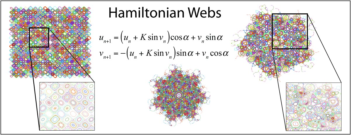
The Hamiltonian of the periodically kicked harmonic oscillator is converted into the Web Map, represented as an iterative mapping as

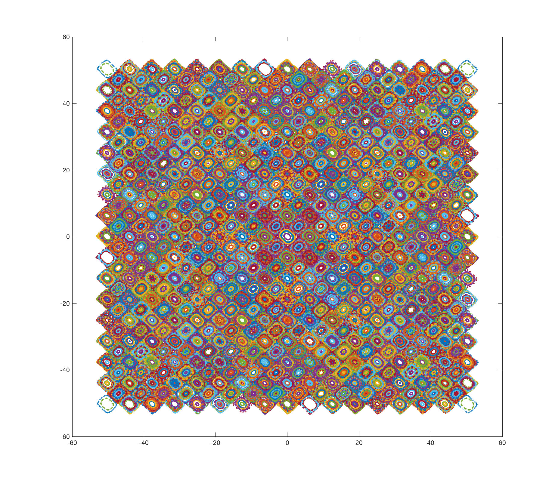
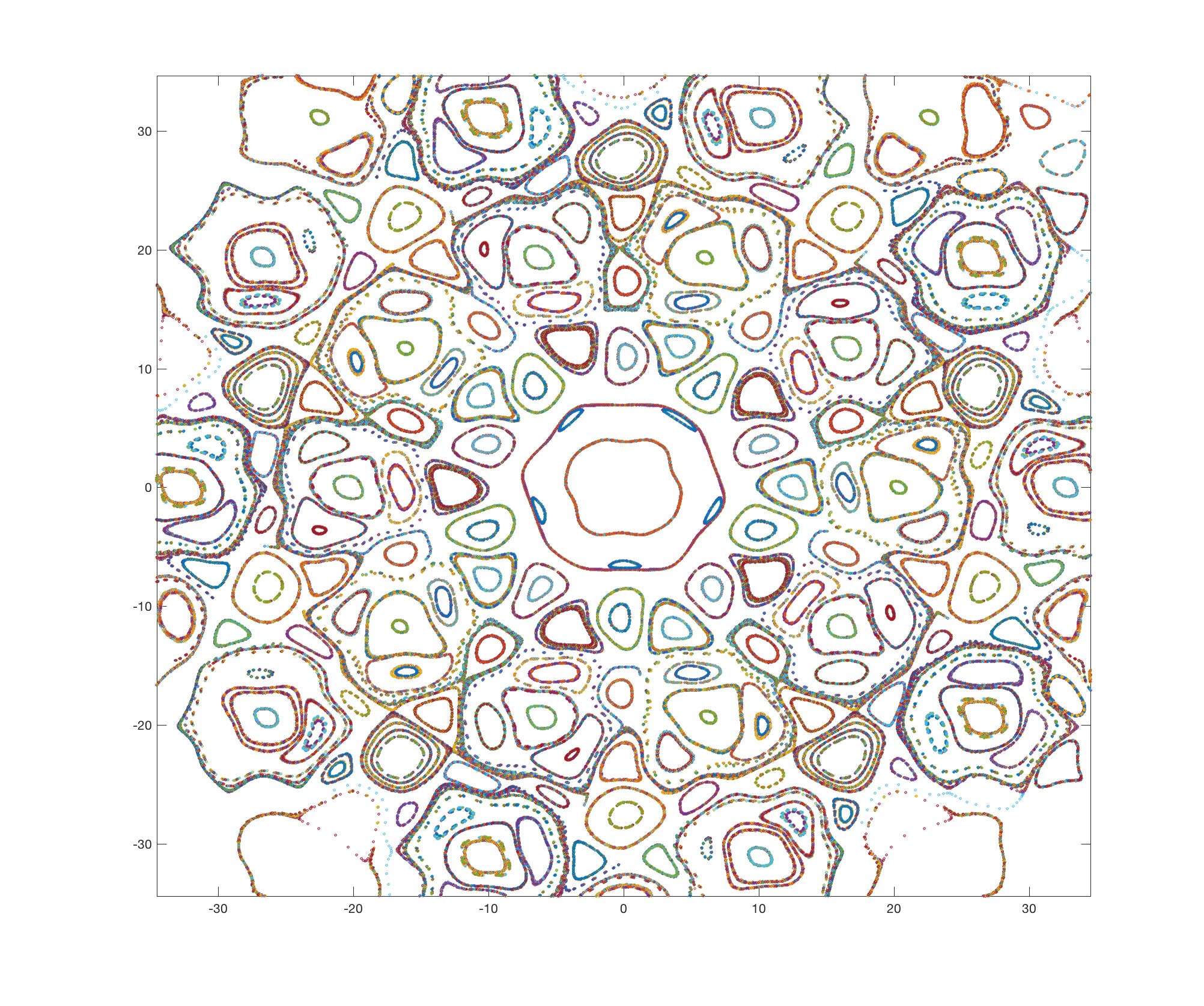
There can be resonance between the sequence of kicks and the natural oscillator frequency such that α = 2π/q. At these resonances, intricate web patterns emerge. The Web Map produces a web of stochastic layers when plotted on an extended phase plane. The symmetry of the web is controlled by the integer q, and the stochastic layer width is controlled by the perturbation strength K.
See simulations for q = 3, 4, 5, 6 and 7 on Youtube.
Web Map Matlab Program
Iterated maps are easy to implement in code. Here is a simple Matlab code to generate maps of different types. (The Python code is on GitHub.) You can play with the coupling constant K and the periodicity q. For small K, the tapestries are mostly regular. But as the coupling K increases, stochastic layers emerge. When q is a small even number, tapestries of regular symmetric are generated. However, when q is an odd small integer, the tapestries turn into quasi-crystals.
% webmap.m

clear
format compact
close all

phi = (1+sqrt(5))/2;

K = phi-1;      % (0.618, 4) (0.618,5) (0.618,7) (1.2, 4)
q = 7;          % 4
alpha = 2*pi/q;
h1 = figure(1);
h1.Position = [177 1 962 804];
dum = set(h1);
axis square

for loop = 1:2000       % 4000

    ulast = 50*rand;   % 50*rand
    vlast = 50*rand;

    for loop = 1:300     % 300

        u(loop) = (ulast + K*sin(vlast))*cos(alpha) + vlast*sin(alpha);
        v(loop) = -(ulast + K*sin(vlast))*sin(alpha) + vlast*cos(alpha);

        ulast = u(loop);
        vlast = v(loop);
    end

    figure(1)
    plot(u,v,'o','MarkerSize',2)
    hold on

end

set(gcf,'Color','white')
%axis([-20 20 -20 20])
axis off
References and Further Reading
D. D. Nolte, Introduction to Modern Dynamics: Chaos, Networks, Space and Time (Oxford, 2015)
G. M. Zaslavsky, Hamiltonian chaos and fractional dynamics. (Oxford, 2005)
This Blog Post is a Companion to the undergraduate physics textbook Modern Dynamics: Chaos, Networks, Space and Time, 2nd ed. (Oxford, 2019) introducing Lagrangians and Hamiltonians, chaos theory, complex systems, synchronization, neural networks, econophysics and Special and General Relativity.


[…] Introductory physics classes emphasize the conservation of energy, linear momentum and angular momentum as if they are special cases. Yet there is a grand structure that yields a universal set of conservation laws: integrable Hamiltonian systems. An integrable system is one for which there are as many invariants of motion as there are degrees of freedom. Amazingly, these conservation laws can all be captured by a single procedure known as (canonical) transformation to action-angle coordinates. When expressed in action-angle form, these Hamiltonians take on extremely simple expressions. They are also the starting point for the study of perturbations when small nonintegrable terms are added to the Hamiltonian. As the perturbations grow, this provides one doorway to the emergence of chaos. […]
LikeLike
[…] How to Weave a Tapestry from Hamiltonian Chaos […]
LikeLike
[…] How to Weave a Tapestry from Hamiltonian Chaos […]
LikeLike
[…] How to Weave a Tapestry from Hamiltonian Chaos […]
LikeLike
[…] How to Weave a Tapestry from Hamiltonian Chaos […]
LikeLike
[…] Schwarzschild was intrigued by Ehrenfest’s paper on adiabatic invariants and their similarity to several of the invariant theorems of Poincaré that he had studied for his doctorate. Up until this time, mechanics had been mostly pursued through the Lagrangian formalism which could easily handle generalized forces associated with dissipation. But celestial mechanics are conservative systems for which the Hamiltonian formalism is a more natural approach. In particular, the Hamilton-Jacobi canonical transformations made it particularly easy to find pairs of generalized coordinates that had simple periodic behavior. In his published paper [9], Schwarzschild called these “Action-Angle” coordinates because one was the action integral that was well-known in the principle of “Least Action”, and the other was like an angle variable that changed steadily in time (see Fig. 5). Action-angle coordinates have come to form the foundation of many of the properties of Hamiltonian chaos, Hamiltonian maps, and Hamiltonian tapestries. […]
LikeLike
[…] How to Weave a Tapestry from Hamiltonian Chaos […]
LikeLike
[…] How to Weave a Tapestry from Hamiltonian Chaos […]
LikeLike
[…] How to Weave a Tapestry from Hamiltonian Chaos […]
LikeLike