Maxwellian Steampunk and the Origins of Maxwell’s Equations

Physicists of the nineteenth century were obsessed with mechanical models.  They must have dreamed, in their sleep, of spinning flywheels connected by criss-crossing drive belts turning enmeshed gears.  For them, Newton’s clockwork universe was more than a metaphor—they believed that mechanical description of a phenomenon could unlock further secrets and act as a tool of discovery. 

It is no wonder they thought this way—the mid-eighteenth century was at the peak of the industrial revolution, dominated by the steam engine and the profusion of mechanical power and gears across broad swaths of society. 
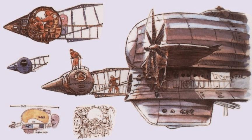
Steampunk

The Victorian obsession with steam and power is captured beautifully in the literary and animé genre known as Steampunk.  The genre is alternative historical fiction that portrays steam technology progressing into grand and wild new forms as electrical and gasoline technology fail to develop.  An early classic in the genre is Miyazaki’s 1986 anime´ film Castle in the Sky (1986) by Hayao Miyazaki about a world where all mechanical devices, including airships, are driven by steam.  A later archetype of the genre is the 2004 animé film Steam Boy (2004) by Katsuhiro Otomo about the discovery of superwater that generates unlimited steam power.  As international powers vie to possess it, mad scientists strive to exploit it for society, but they create a terrible weapon instead.   One of the classics that helped launch the genre is the novel The Difference Engine (1990) by William Gibson and Bruce Sterling that envisioned an alternative history of computers developed by Charles Babbage and Ada Lovelace.

Scenes from Miyazaki's Castle in the Sky.

Steampunk is an apt, if excessively exaggerated, caricature of the Victorian mindset and approach to science.  Confidence in microscopic mechanical models among natural philosophers was encouraged by the success of molecular models of ideal gases as the foundation for macroscopic thermodynamics.  Pictures of small perfect spheres colliding with each other in simple billiard-ball-like interactions could be used to build up to overarching concepts like heat and entropy and temperature.  Kinetic theory was proposed in 1857 by the German physicist Rudolph Clausius and was quickly placed on a firm physical foundation using principles of Hamiltonian dynamics by the British physicist James Clerk Maxwell.
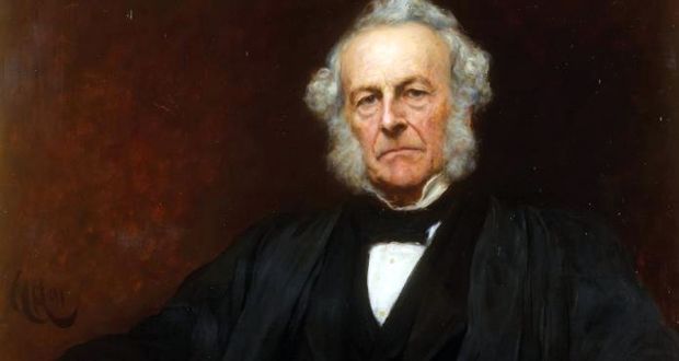
DVD cover of Steamboy by Otomo.

James Clerk Maxwell

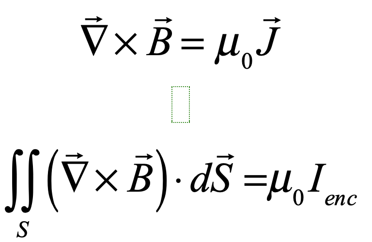
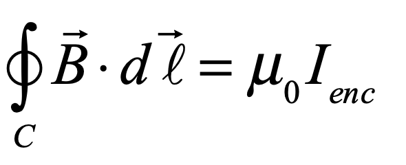
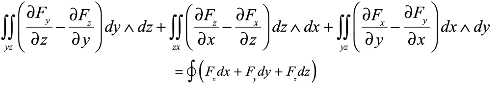
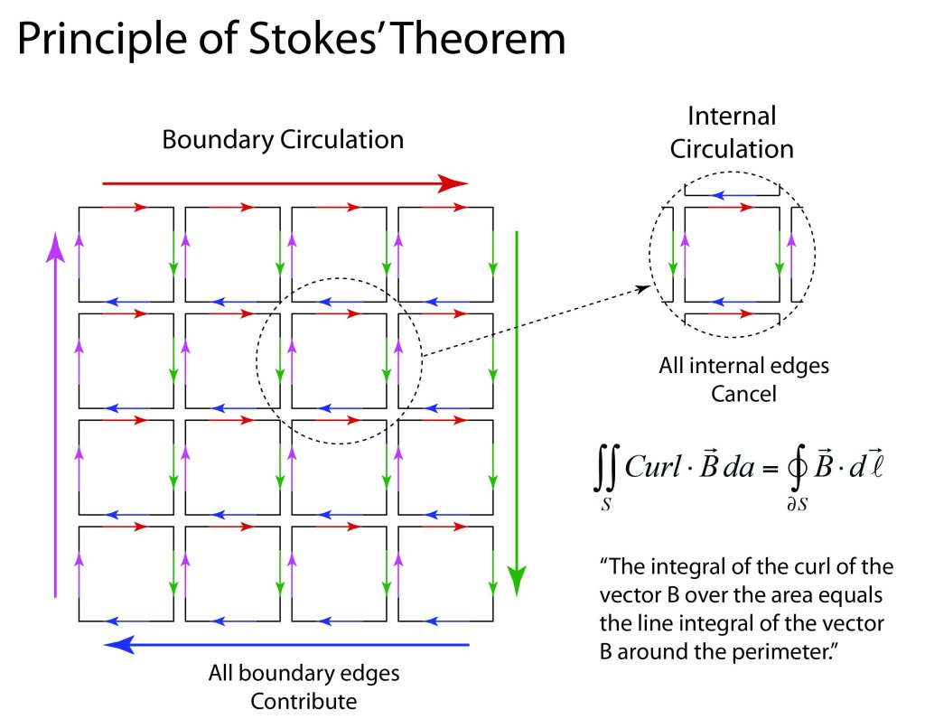
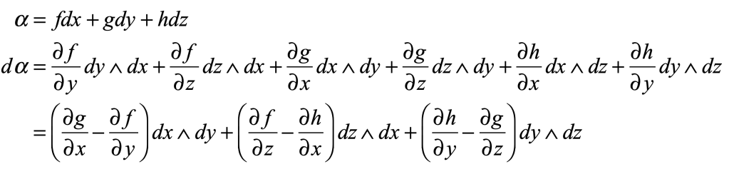
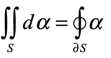
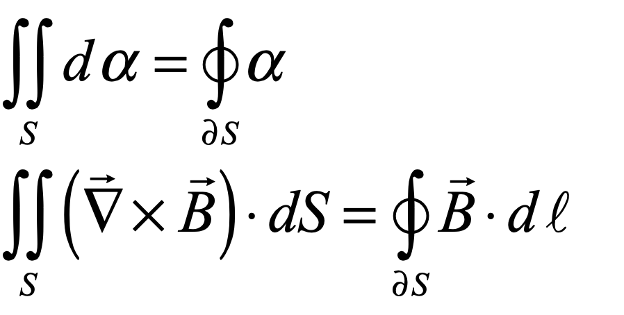
James Clerk Maxwell (1831 – 1879) was one of three titans out of Cambridge who served as the intellectual leaders in mid-nineteenth-century Britain. The two others were George Stokes and William Thomson (Lord Kelvin).  All three were Wranglers, the top finishers on the Tripos exam at Cambridge, the grueling eight-day examination across all fields of mathematics.  The winner of the Tripos, known as first Wrangler, was announced with great fanfare in the local papers, and the lucky student was acclaimed like a sports hero is today.  Stokes in 1841 was first Wrangler while Thomson (Lord Kelvin) in 1845 and Maxwell in 1854 were each second Wranglers.  They were also each winners of the Smith’s Prize, the top examination at Cambridge for mathematical originality.  When Maxwell sat for the Smith’s Prize in 1854 one of the exam problems was a proof written by Stokes on a suggestion by Thomson.  Maxwell failed to achieve the proof, though he did win the Prize.  The problem became known as Stokes’ Theorem, one of the fundamental theorems of vector calculus, and the proof was eventually provided by Hermann Hankel in 1861.

James Clerk Maxwell.

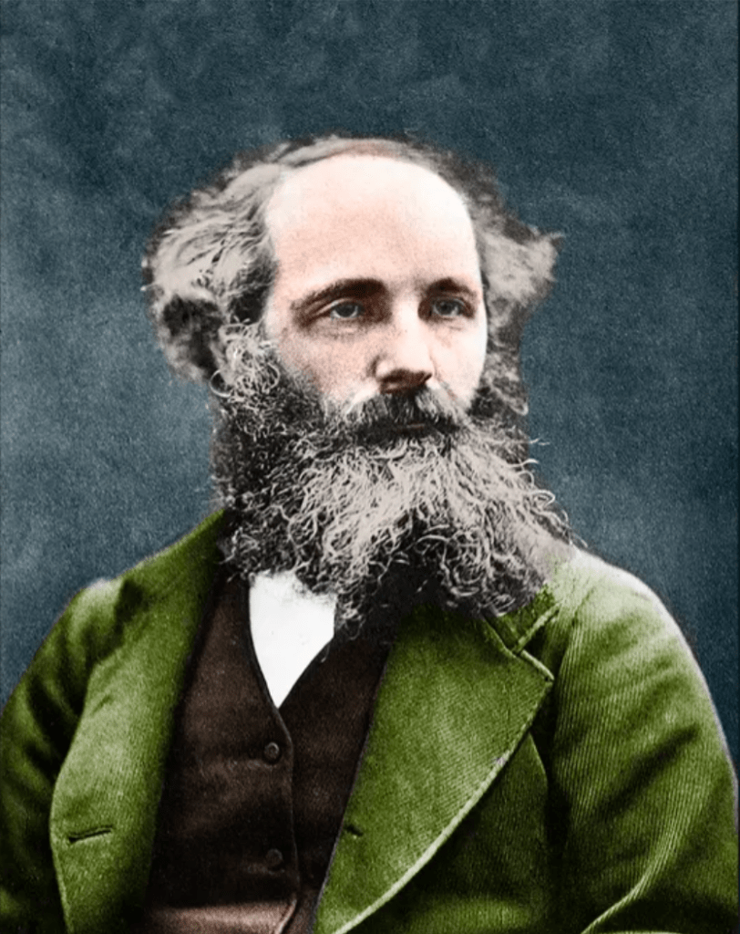
After graduation from Cambridge, Maxwell took the chair of natural philosophy at Marischal College in the city of Aberdeen in Scotland.  He was only 25 years old when he began, fifteen years younger than any of the other professors.  He split his time between the university and his family home at Glenlair in the south of Scotland, which he inherited from his father the same year he began his chair at Aberdeen.  His research interests spanned from the perception of color to the rings of Saturn.  He improved on Thomas Young’s three-color theory by correctly identifying red, green and blue as the primary receptors of the eye and invented a scheme for adding colors that is close to the HSV (hue-saturation-value) system used today in computer graphics.  In his work on the rings of Saturn, he developed a statistical mechanical approach to explain how the large-scale structure emerged from the interactions among the small grains.  He applied these same techniques several years later to the problem of ideal gases when he derived the speed distribution known today as the Maxwell-Boltzmann distribution.

Maxwell’s career at Aberdeen held great promise until he was suddenly fired from his post in 1860 when Marischal College merged with nearby King’s College to form the University of Aberdeen.  After the merger, the university had the abundance of two professors of Natural Philosophy while needing only one, and Maxwell was the junior.  With his new wife, Maxwell retired to Glenlair and buried himself in writing the first drafts of a paper titled “On Physical Lines of Force” [2].  The paper explored the mathematical and mechanical aspects of the curious lines of magnetic force that Michael Faraday had first proposed in 1831 and which Thomson had developed mathematically around 1845 as the first field theory in physics. 

As Maxwell explored the interrelationships among electric and magnetic phenomena, he derived a wave equation for the electric and magnetic fields and was astounded to find that the speed of electromagnetic waves was essentially the same as the speed of light.  The importance of this coincidence did not escape him, and he concluded that light—that rarified, enigmatic and quintessential fifth element—must be electromagnetic in origin. Ever since Francois Arago and Agustin Fresnel had shown that light was a wave phenomenon, scientists had been searching for other physical signs of the medium that supported the waves—a medium known as the luminiferous aether (or ether). With Maxwell’s new finding, it meant that the luminiferous ether must be related to electric and magnetic fields.  In the Steampunk tradition of his day, Maxwell began a search for a mechanical model.  He did not need to look far, because his friend Thomson had already built a theory on a foundation provided by the Irish mathematician James MacCullagh (1809 – 1847)

The Luminiferous Ether

The late 1830’s was a busy time for the luminiferous ether.  Agustin-Louis Cauchy published his extensive theory of the ether in 1836, and the self-taught George Green published his highly influential mathematical theory in 1838 which contained many new ideas, such as the emphasis on potentials and his derivation of what came to be called Green’s theorem

In 1839 MacCullagh took an approach that established a core property of the ether that later inspired both Thomson and Maxwell in their development of electromagnetic field theory.  What McCullagh realized was that the energy of the ether could be considered as if it had both kinetic energy and potential energy (ideas and nomenclature that would come several decades later).  Most insightful was the fact that the potential energy of the field depended on pure rotation like a vortex.  This rotationally elastic ether was a mathematical invention without any mechanical analog, but it successfully described reflection and refraction as well as polarization of light in crystalline optics. 

In 1856 Thomson put Faraday’s famous magneto-optic rotation of light (the Faraday Effect discovered by Faraday in 1845) into mathematical form and began putting Faraday’s initially abstract ideas of the theory of fields into concrete equations.  He drew from MacCullagh’s rotational ether as well as an idea from William Rankine about the molecular vortex model of atoms to develop a mechanical vortex model of the ether.  Thomson explained how the magnetic field rotated the linear polarization of light through the action of a multiplicity of molecular vortices.  Inspired by Thomson, Maxwell took up the idea of molecular vortices as well as Faraday’s magnetic induction in free space and transferred the vortices from being a property exclusively of matter to being a property of the luminiferous ether that supported the electric and magnetic fields. 

Maxwellian Cogwheels

Maxwell’s model of the electromagnetic fields in the ether is the apex of Victorian mechanistic philosophy—too explicit to be a true model of reality—yet it was amazingly fruitful as a tool of discovery, helping Maxwell develop his theory of electrodynamics. The model consisted of an array of elastic vortex cells separated by layers of small particles that acted as “idle wheels” to transfer spin from one vortex to another .  The magnetic field was represented by the rotation of the vortices, and the electric current was represented by the displacement of the idle wheels. 

Maxwell's vortex model
Fig. 1 Maxwell’s vortex model of the electromagnetic ether.  The molecular vortices rotate according to the direction of the magnetic field, supported by idle wheels.  The physical displacement of the idle wheels became an analogy for Maxwell’s displacement current [2].

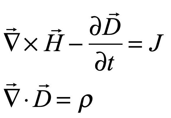
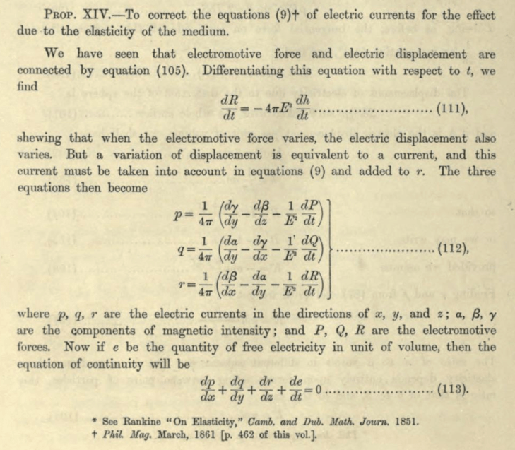
Two predictions by this outrightly mechanical model were to change the physics of electromagnetism forever:  First, any change in strain in the electric field would cause the idle wheels to shift, creating a transient current that was called a “displacement current”.  This displacement current was one of the last pieces in the electromagnetic puzzle that became Maxwell’s equations. 

Maxwell's discovery of the displacement current
Fig. 2 In “Physical Lines of Force” in 1861, Maxwell introduces the idea of a displacement current [RefLink].

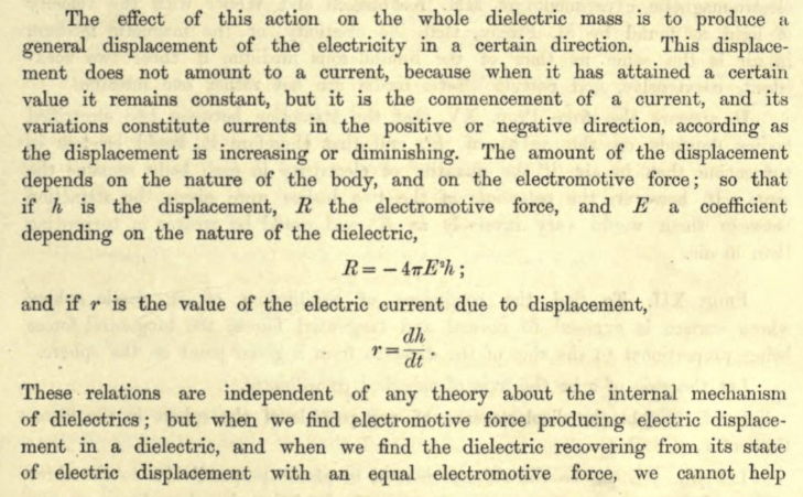
In this description, E is not the electric field, but is related to the dielectric permativity through the relation

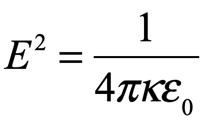
Maxwell went further to prove his Proposition XIV on the contribution of the displacement current to conventional electric currents.

Maxwell completing the laws of electromagnetics
Fig. 3 Maxwell’s Proposition XIV on adding the displacement current to the conventional electric current [RefLink].

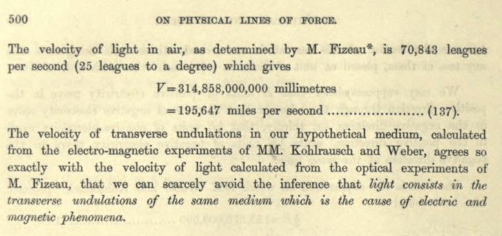
Second, Maxwell calculated that this elastic vortex ether propagated waves at a speed that was close to the known speed of light measured a decade previously by the French physicist Hippolyte Fizeau.  He remarked, “we can scarcely avoid the inference that light consists of the transverse undulations of the same medium which is the cause of electric and magnetic phenomena.” [1]  This was the first direct prediction that light, previously viewed as a physical process separate from electric and magnetic fields, was an electromagnetic phenomenon.

Maxwell's estimate of the speed of light
Fig. 4 Maxwell’s calculation of the speed of light in his mechanical ether. It matched closely the measured speed of light [RefLink].

These two predictions—of the displacement current and the electromagnetic origin of light—have stood the test of time and are center pieces of Maxwells’s legacy.  How strange that they arose from a mechanical model of vortices and idle wheels like so many cogs and gears in the machinery powering the Victorian age, yet such is the power of physical visualization.


[1] pg. 12, The Maxwellians, Bruce Hunt (Cornell University Press, 1991)

[2] Maxwell, J. C. (1861). “On physical lines of force”. Philosophical Magazine. 90: 11–23.

Books by David Nolte at Oxford University Press

Looking Under the Hood of the Generalized Stokes Theorem

Everyone who has taken classes in physics or engineering knows that the most magical of all vector identities (and there are so many vector identities) are Green’s theorem in 2D, and Stokes’ and Gauss’ theorem in 3D.  These theorems have the magical ability to take an integral over some domain and replace it with a simpler integral over the boundary of the domain.  For instance, the vector form of Stokes’ theorem in 3D is

for the curl of a vector field, where S is the surface domain, and C is the closed loop surrounding the domain.

Maybe the most famous application of these theorems is to convert Maxwell’s equations of electromagnetism from their differential form to their integral form.  For instance, we can start with the differential version for the curl of the B-field and integrate over a surface

then applying Stokes’ theorem in 3D (or Green’s theorem in 2D), that converts from the two-dimensional surface integral to a one-dimensional integral around a closed loop bounding the area integral domain yields the integral form of Ampere’s law

Stokes’ theorem has the important property that it converts a high-dimensional integral into a lower-dimensional integral over the closed boundary of the original domain. Stokes’ theorem in component form is

where the “hat” symbol is Grassmann’s wedge product (see below). In the case of Green’s theorem in 2D, the principle is easy to explain by the oriented vector character of the integrals and the notion of dividing a domain into small elements with oriented edges. In the case of nonzero circulation, all internal edges of smaller regions cancel pairwise until the outer boundary is reached, where a macroscopic circulation persists along all the outer edges. Similarly in Gauss’ theorem in 3D, the flux of a vector through the face of one element is equal and opposite to the flux through the adjacent element, canceling out pairwise until the outer boundary is reached and the net flux is finite summed over the outer elements. This general property of pairwise cancelation on adjacent subdomains until the outer boundary is reached is the general property of Stokes’ theorem that can be extended to space of any dimensions or onto general manifolds that do not need to be Euclidean.

Figure. Principle of Stokes’ theorem. The circulation from all internal edges cancels out. But on the boundary, all edges add together for a macroscopic circulation.

George Stokes and the Cambridge Tripos

Since 1824, the mathematics course at Cambridge University has held a yearly exam called the Tripos to identify the top graduating mathematics student.  The winner of the contest is called the Senior Wrangler, and in the 1800’s the Senior Wrangler received a level of public fame and admiration for intellectual achievement that is somewhat like the fame reserved today for star athletes.  Famous Senior Wranglers include George Airy, John Herschel, Arthur Cayley, Lord Rayleigh, Arthur Eddington, J. E. Littlewood, Peter Guthrie Tait and Joseph Larmor.

Figure. Sir George Gabriel Stokes, 1st Baronet

            In his second year at Cambridge, Stokes had begun studying under William Hopkins (1793 – 1866), and in 1841 George Stokes became Senior Wrangler the same year he won the Smith’s Prize in mathematics.  The Tripos tested primarily on bookwork, while the Smith’s Prize tested on originality.  To achieve top scores on both designated the student as the most capable and creative mathematician of his class.  Stokes was immediately offered a fellowship at Pembroke College allowing him to teach and study whatever he willed. Within eight years he was chosen for the Lucasian Chair of Mathematics. The Lucasian Chair of Mathematics at Cambridge is one of the most famous academic chairs in the world.  The first Lucasian professor was Isaac Barrow in 1664 followed by Isaac Newton who held the post for 33 years.  Other famous Lucasian professors were George Airy, Charles Babbage, Joseph Larmor, Paul Dirac as well as Stephen Hawking. Among the many fields that Stokes made important contributions was hydrodynamics where he derived Stokes’ Law of Drag.

In 1854 Stokes was one of the Cambridge professors setting exam questions for the Tripos. In a letter that William Thompson (later Lord Kelvin) wrote Stokes, he suggested putting on the exam the task of extending Green’s Theorem to three dimensions and proving the theorem, and Stokes obliged. That year the Tripos consisted of 16 papers spread over 8 days, totaling over 40 hours of effort on 211 questions. One of the candidates for Senior Wrangler that year was James Clerk Maxwell, but he was narrowly beaten out by Edward Routh (1831 – 1907). Routh became famous, but not as famous as Maxwell who later applied Stokes’ Theorem to derive the equations of electrodynamics.

The Fundamental Theorem of Calculus

One of the first and simplest theorems that any student of intro calculus is taught is the Fundamental Theorem of Calculus

where F is called the “antiderivative” of the function f . The interpretation of the Fundamental Theorem is extremely simple:  The integral of a function over a domain is equal to its antiderivative evaluated at the boundary of the domain.  Generalizing this theorem a bit, it says that evaluating an integral over a domain is the same thing as evaluating a lower-dimensional quantity over the boundary of the domain.  The Fundamental Theorem of Calculus sounds a lot like Green’s Theorem or Stokes’ Theorem!  And in fact, they are all part of the same principle.  To understand this principle, we have to look into differential forms and the use of Grassmann’s wedge product and exterior algebra (the subject of my previous blog post).

Differential Forms

Just as in the case of the exterior algebra , the fundamental identities defined for differential forms are given by

A differential 1-form α and a differential 2-form β can be expressed as

The key to understanding why the wedge product shows up in this definition is to recognize that the operation of producing a product of differentials is only defined for the wedge product.  Within the language of differential forms, the symbol dxdy has no meaning, despite the fact that this symbol shows up routinely when integrating.  In fact, integrals that use the expression dxdy are ambiguous, because the oriented surface must be inferred from the context of the integral rather than given.  This is why integration over multiple variables should actually be performed using differential forms, though it is rarely (or never) stated in lower-level calculus classes.

Integration of Differential Forms

Line integrals, as in the Fundamental Theorem of Calculus, are obvious and unique.  However, as soon as we move to integrals over areas, the wedge product is needed.  This is because a general area is oriented.  If you think of a plane defined by z = 0, the surface element dxdy can be oriented along either the positive z-axis or the negative z-axis.  Which one should you take?  The answer is: don’t make the choice.  Work with differential forms, and the integral may be over dx^dy or dy^dx, depending on the exterior analysis that produced the integral in the first place.  One is the negative of the other.  You take the element as it arises from the algebra, and you cannot go wrong!

As an example, we can use differential forms to express a surface integral correctly as

If you make the substitutions: x = (p-q)/2 and y = (p+q)/2, then dp = dx + dy and dq = dy – dx and

which yields

In this case, you will recognize that the factor of -2 is just the Jacobian of the transformation.  Working this way with differential forms makes transformation simple, like a book-keeping trick, and safe, so you just follow the algebra through without needing to make choices.

Exterior Differentiation

The exterior derivative of the 1-form α (defined above) is defined as

where the exterior derivative turns a differential r-form into a differential (r+1)-form.  For instance, in 3D

This should look very familiar to you.  If we expressly make the equivalence

where the integral on the left is a surface integral over a domain, and the integral on the right is a line integral over a line bounding the domain, then

This is just the curl theorem (Stokes’ theorem).

Figure. Stokes Theorem in 3D vector form and general form.

Taking the dimension up one notch, consider the differential 2-form β where

This again looks very familiar, and if we write down the equivalence

then we immediately have the divergence theorem.

We can even find other vector identities using these differential forms.  For instance, if we start with a 2-form expressed as

then we have proven the vector identity

stating that the divergence of a curl must vanish.  This is like playing games with simple algebra to prove profound theorems in vector calculus!

Figure. Exterior differentiation of a differential 1-form to yield a differential 2-form.

Stokes’ Theorem in Higher Dimensions

The power of differential forms is their ability to generalize automatically to higher dimensions. The differential 1-form can have any number of indices for multiple dimensions, and exterior differentiation yields the familiar curl theorem in any number of dimensions

But the differential 2-form in 4D yields to exterior differentiation to give a mixed expression that is neither a curl nor a divergence

The differential 3-form in 4D under exterior differentiation yields the 4D divergence

although the orientations of the 3D boundary elements must be chosen appropriately.

Differential Forms in 4D Electromagnetics

As long as we are working with differential forms and Stokes’ Theorem, let’s finish up by looking at Maxwell’s electromagnetic equations as four-dimensional equations in spacetime.  First, construct the 2-form using the displacement field D and the magnetic intensity H.

The differential of this two-form creates a lot of terms, such as

This can be simplified by collecting like terms to

Renaming each coefficient so that

yields two of Maxwell’s equations

To find the other two Maxwell equations, start with the 1-form

and try the derivation yourself!

Differentiating yields a differential two-form. Then identify the curl of the vector potential as the B-field, etc., to derive the other two Maxwell equations

Bibliography

Vargas, J. G., Differential Geometry for Physicists and Mathematicians: Moving Frames and Differential Forms: From Euclid Past Riemann. 2014; p 1-293.