Of all the audacious proposals made by Einstein, and there were many, this one takes the cake because it should be impossible.
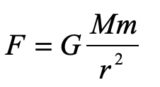
There can be no force of gravity on light because light has no mass. Without mass, there is no gravitational “interaction”. We all know Newton’s Law of gravity … it was one of the first equations of physics we ever learned
which shows the interaction between the masses M and m through their product. For light, this is strictly zero.
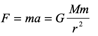
How, then did Einstein conclude, in 1907, only two years after he proposed his theory of special relativity, that gravity bends light? If it were us, we might take Newton’s other famous equation and equate the two
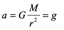
and guess that somehow the little mass m (though it equals zero) cancels out to give
so that light would fall in gravity with the same acceleration as anything else, massive or not.
But this is not how Einstein arrived at his proposal, because this derivation is wrong! To do it right, you have to think like an Einstein.
“My Happiest Thought”
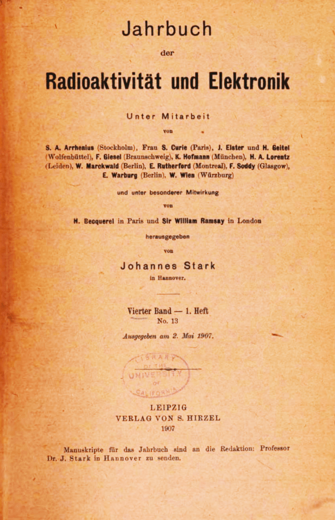
Towards the end of 1907, Einstein was asked by Johannes Stark to contribute a review article on the state of the relativity theory to the Jahrbuch of Radioactivity and Electronics. There had been a flurry of activity in the field in the two years since Einstein had published his groundbreaking paper in Annalen der Physik in September of 1905 [1]. Einstein himself had written several additional papers on the topic, along with others, so Stark felt it was time to put things into perspective.
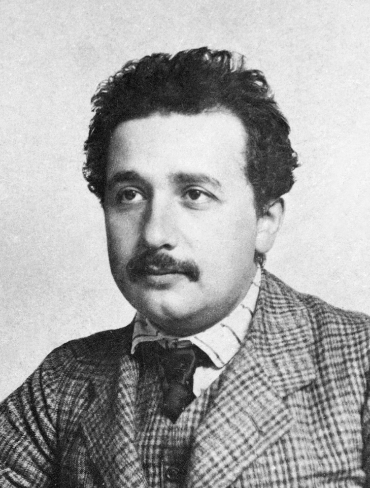
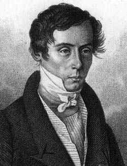
Fig. 1 Einstein around 1905.
Einstein was still working at the Patent Office in Bern, Switzerland, which must not have been too taxing, because it gave him plenty of time think. It was while he was sitting in his armchair in his office in 1907 that he had what he later described as the happiest thought of his life. He had been struggling with the details of how to apply relativity theory to accelerating reference frames, a topic that is fraught with conceptual traps, when he had a flash of simplifying idea:
“Then there occurred to me the ‘glucklichste Gedanke meines Lebens,’ the happiest thought of my life, in the following form. The gravitational field has only a relative existence in a way similar to the electric field generated by magnetoelectric induction. Because for an observer falling freely from the roof of a house there exists —at least in his immediate surroundings— no gravitational field. Indeed, if the observer drops some bodies then these remain relative to him in a state of rest or of uniform motion… The observer therefore has the right to interpret his state as ‘at rest.'”[2]
In other words, the freely falling observer believes he is in an inertial frame rather than an accelerating one, and by the principle of relativity, this means that all the laws of physics in the accelerating frame must be the same as for an inertial frame. Hence, his great insight was that there must be complete equivalence between a mechanically accelerating frame and a gravitational field. This is the very first conception of his Equivalence Principle.
Fig. 2 Front page of the 1907 volume of the Jahrbuch. The editor list reads like a “Whos-Who” of early modern physics.
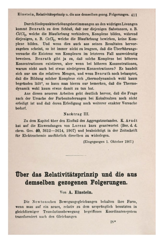
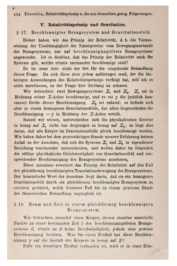
After completing his review of the consequences of special relativity in his Jahrbuch article, Einstein took the opportunity to launch into his speculations on the role of the relativity principle in gravitation. He is almost appologetic at the start, saying that:
“This is not the place for a detailed discussion of this question. But as it will occur to anybody who has been following the applications of the principle of relativity, I will not refrain from taking a stand on this question here.”
But he then launches into his first foray into general relativity with keen insights.
Fig. 4 The beginning of the section where Einstein first discusses the effects of accelerating frames and effects of gravity.
He states early in his exposition:
“… in the discussion that follows, we shall therefore assume the complete physical equivalence of a gravitational field and a corresponding accelerated reference system.”
Here is his equivalence principle. And using it, in 1907, he derives the effect of acceleration (and gravity) on ticking clocks, on the energy density of electromagnetic radiation (photons) in a gravitational potential, and on the deflection of light by gravity.
Over the next several years, Einstein was distracted by other things, such as obtaining his first university position, and his continuing work on the early quantum theory. But by 1910 he was ready to tackle the general theory of relativity once again, when he discovered that his equivalence principle was missing a key element: the effects of spatial curvature, which launched him on a 5-year program into the world of tensors and metric spaces that culminated with his completed general theory of relativity that he published in November of 1915 [4].
The Observer in the Chest: There is no Elevator
Einstein was never a stone to gather moss. Shortly after delivering his triumphal exposition on the General Theory of Relativity, he wrote up a popular account of his Special and now General Theories to be published as a book in 1916, first in German [5] and then in English [6]. What passed for a “popular exposition” in 1916 is far from what is considered popular today. Einstein’s little book is full of equations that would be somewhat challenging even for specialists. But the book also showcases Einstein’s special talent to create simple analogies, like the falling observer, that can make difficult concepts of physics appear crystal clear.
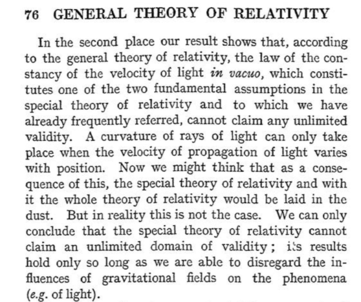
In 1916, Einstein was not yet thinking in terms of an elevator. His mental image at this time, for a sequestered observer, was someone inside a spacious chest filled with measurement apparatus that the observer could use at will. This observer in his chest was either floating off in space far from any gravitating bodies, or the chest was being pulled by a rope hooked to the ceiling such that the chest accelerates constantly. Based on the measurement he makes, he cannot distinguish between gravitational fields and acceleration, and hence they are equivalent. A bit later in the book, Einstein describes what a ray of light would do in an accelerating frame, but he does not have his observer attempt any such measurement, even in principle, because the deflection of the ray of light from a linear path would be far too small to measure.
But Einstein does go on to say that any curvature of the path of the light ray requires that the speed of light changes with position. This is a shocking admission, because his fundamental postulate of relativity from 1905 was the invariance of the speed of light in all inertial frames. It was from this simple assertion that he was eventually able to derive E = mc2. Where, on the one hand, he was ready to posit the invariance of the speed of light, on the other hand, as soon as he understood the effects of gravity on light, Einstein did not hesitate to cast this postulate adrift.
Fig. 5 Einstein’s argument for the speed of light depending on position in a gravitational field.
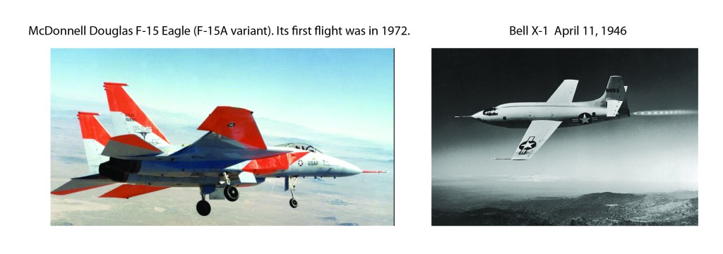
(Einstein can be forgiven for taking so long to speak in terms of an elevator that could accelerate at a rate of one g, because it was not until 1946 that the rocket plane Bell X-1 achieved linear acceleration exceeding 1 g, and jet planes did not achieve 1 g linear acceleration until the F-15 Eagle in 1972.)
Fig. 6 Aircraft with greater than 1:1 thrust to weight ratios.
The Evolution of Physics: Enter Einstein’s Elevator
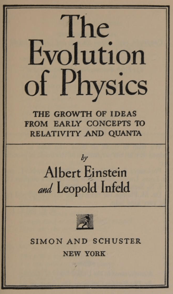
Years passed, and Einstein fled an increasingly autocratic and belligerent Germany for a position at Princeton’s Institute for Advanced Study. In 1938, at the instigation of his friend Leopold Infeld, they decided to write a general interest book on the new physics of relativity and quanta that had evolved so rapidly over the past 30 years.
Fig. 7 Title page of “Evolution of Physics” 1938 written with his friend Leopold Infeld at Princeton’s Institute for Advanced Study.
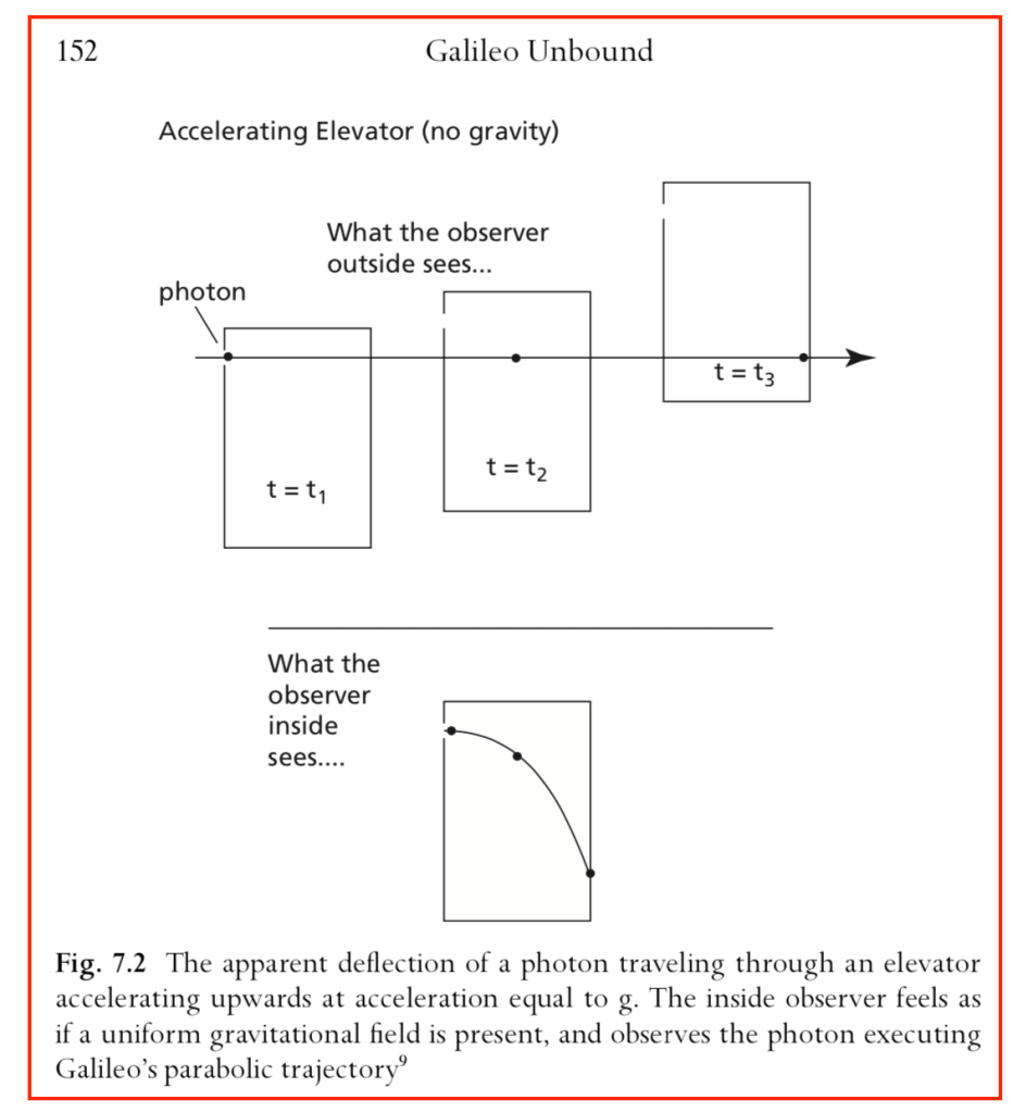
Here, in this obscure book that no-one remembers today, we find Einstein’s elevator for the first time, and the exposition talks very explicitly about a small window that lets in a light ray, and what the observer sees (in principle) for the path of the ray.
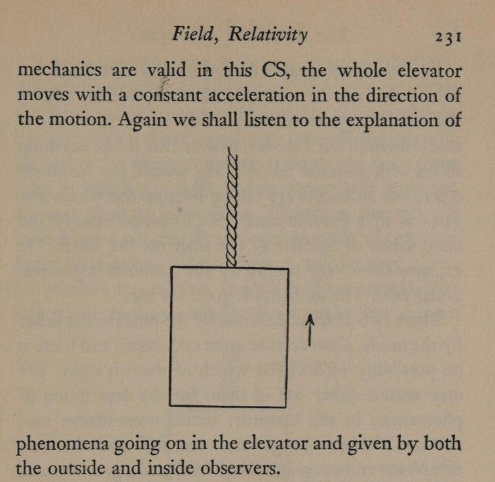
Fig. 8 One of the only figures in the Einstein and Infeld book: The origin of “Einstein’s Elevator”!
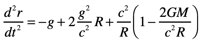
By the equivalence principle, the observer cannot tell whether they are far out in space, being accelerated at the rate g, or whether they are statinary on the surface of the Earth subject to a gravitational field. In the first instance of the accelerating elevator, a photon moving in a straight line through space would appear to deflect downward in the elevator, as shown in Fig. 9, because the elevator is accelerating upwards as the photon transits the elevator. However, by the equivalence principle, the same physics should occur in the gravitational field. Hence, gravity must bend light. Furthermore, light falls inside the elevator with an acceleration g, just as any other object would.
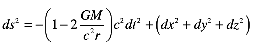
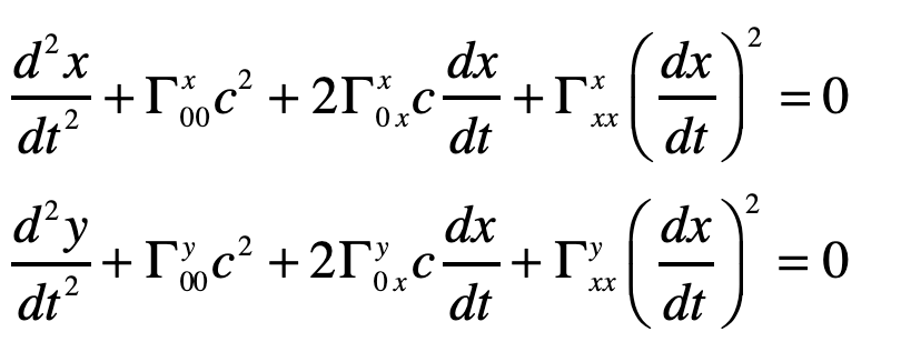
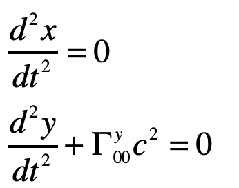
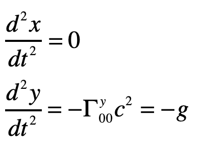
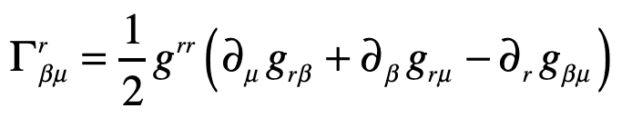
A photon enters an elevator at right angles to its acceleration vector g. Use the geodesic equation and the elevator (Equivalence Principle) metric [8]
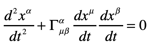
The geodesic equation with time as the dependent variable
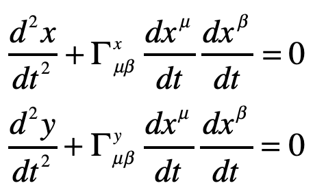
This gives two coordinate equations
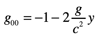
Note that x0 = ct and x1 = ct are both large relative to the y-motion of the photon. The metric component that is relevant here is
and the others are unity. The geodesic becomes (assuming dy/dt = 0)
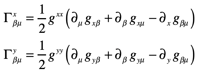
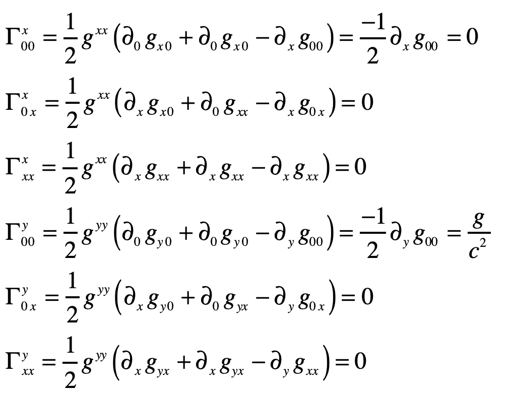
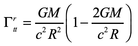
The Christoffel symbols are
which give
Therefore
or
where the photon falls with acceleration g, as anticipated.
Light Deflection in the Schwarzschild Metric
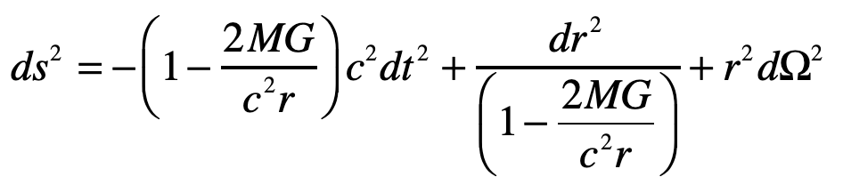
Do the same problem of the light ray in Einstein’s Elevator, but now using the full Schwarzschild solution to the Einstein Field equations.
Solution:
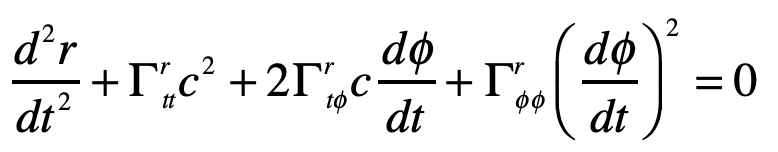
Einstein’s elevator is the classic test of virtually all heuristic questions related to the deflection of light by gravity. In the previous Example, the deflection was attributed to the Equivalence Principal in which the observer in the elevator cannot discern whether they are in an acceleration rocket ship or standing stationary on Earth. In that case, the time-like metric component is the sole cause of the free-fall of light in gravity. In the Schwarzschild metric, on the other hand, the curvature of the field near a spherical gravitating body also contributes. In this case, the geodesic equation, assuming that dr/dt = 0 for the incoming photon, is
where, as before, the Christoffel symbol for the radial displacements are
Evaluating one of these
The other Christoffel symbol that contributes to the radial motion is
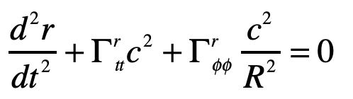
and the geodesic equation becomes
with
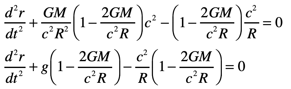
The radial acceleration of the light ray in the elevator is thus
The first term on right is free-fall in gravity, just as was obtained from the Equivalence Principal. The second term is a higher-order correction caused by curvature of spacetime. The third term is the motion of the light ray relative to the curved ceiling of the elevator in this spherical geometry and hence is a kinematic (or geometric) artefact. (It is interesting that the GR correction on the curved-ceiling correction is of the same order as the free-fall term, so one would need to be very careful doing such an experiment … if it were at all measurable.) Therefore, the second and third terms are curved-geometry effects while the first term is the free fall of the light ray.
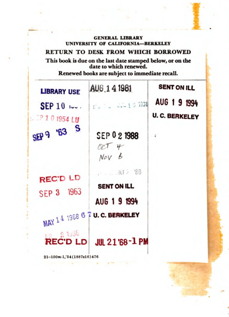
Post-Script: The Importance of Library Collections
I was amused to see the library card of the scanned Internet Archive version of Einstein’s Jahrbuch article, shown below. The volume was checked out in August of 1981 from the UC Berkeley Physics Library. It was checked out again 7 years later in September of 1988. These dates coincide with when I arrived at Berkeley to start grad school in physics, and when I graduated from Berkeley to start my post-doc position at Bell Labs. Hence this library card serves as the book ends to my time in Berkeley, a truly exhilarating place that was the top-ranked physics department at that time, with 7 active Nobel Prize winners on its faculty.
During my years at Berkeley, I scoured the stacks of the Physics Library looking for books and journals of historical importance, and was amazed to find the original volumes of Annalen der Physik from 1905 where Einstein published his famous works. This was the same library where, ten years before me, John Clauser was browsing the stacks and found the obscure paper by John Bell on his inequalities that led to Clauser’s experiment on entanglement that won him the Nobel Prize of 2022.
That library at UC Berkeley was recently closed, as was the Physics Library in my department at Purdue University (see my recent Blog), where I also scoured the stacks for rare gems. Some ancient books that I used to be able to check out on a whim, just to soak up their vintage ambience and to get a tactile feel for the real thing held in my hands, are now not even available through Interlibrary Loan. I may be able to get scans from Internet Archive online, but the palpable magic of the moment of discovery is lost.
References:
[1] Einstein, A. (1905). Zur Elektrodynamik bewegter Körper. Annalen der Physik, 17(10), 891–921.
[2] Pais, A (2005). Subtle is the Lord: The Science and Life of Albert Einstein (Oxford University Press). pg. 178
[3] Einstein, A. (1907). Über das Relativitätsprinzip und die aus demselben gezogenen Folgerungen. Jahrbuch der Radioaktivität und Elektronik, 4, 411–462.
[4] A. Einstein (1915), “On the general theory of relativity,” Sitzungsberichte Der Koniglich Preussischen Akademie Der Wissenschaften, pp. 778-786, Nov.
[5] Einstein, A. (1916). Über die spezielle und die allgemeine Relativitätstheorie (Gemeinverständlich). Braunschweig: Friedr. Vieweg & Sohn.
[6] Einstein, A. (1920). Relativity: The Special and the General Theory (A Popular Exposition) (R. W. Lawson, Trans.). London: Methuen & Co. Ltd.
Physicists of the nineteenth century were obsessed with mechanical models. They must have dreamed, in their sleep, of spinning flywheels connected by criss-crossing drive belts turning enmeshed gears. For them, Newton’s clockwork universe was more than a metaphor—they believed that mechanical description of a phenomenon could unlock further secrets and act as a tool of discovery.
It is no wonder they thought this way—the mid-eighteenth century was at the peak of the industrial revolution, dominated by the steam engine and the profusion of mechanical power and gears across broad swaths of society.
Steampunk
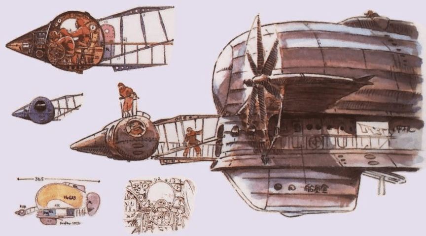
The Victorian obsession with steam and power is captured beautifully in the literary and animé genre known as Steampunk. The genre is alternative historical fiction that portrays steam technology progressing into grand and wild new forms as electrical and gasoline technology fail to develop. An early classic in the genre is Miyazaki’s 1986 anime´ film Castle in the Sky (1986) by Hayao Miyazaki about a world where all mechanical devices, including airships, are driven by steam. A later archetype of the genre is the 2004 animé film Steam Boy (2004) by Katsuhiro Otomo about the discovery of superwater that generates unlimited steam power. As international powers vie to possess it, mad scientists strive to exploit it for society, but they create a terrible weapon instead. One of the classics that helped launch the genre is the novel The Difference Engine (1990) by William Gibson and Bruce Sterling that envisioned an alternative history of computers developed by Charles Babbage and Ada Lovelace.
Steampunk is an apt, if excessively exaggerated, caricature of the Victorian mindset and approach to science. Confidence in microscopic mechanical models among natural philosophers was encouraged by the success of molecular models of ideal gases as the foundation for macroscopic thermodynamics. Pictures of small perfect spheres colliding with each other in simple billiard-ball-like interactions could be used to build up to overarching concepts like heat and entropy and temperature. Kinetic theory was proposed in 1857 by the German physicist Rudolph Clausius and was quickly placed on a firm physical foundation using principles of Hamiltonian dynamics by the British physicist James Clerk Maxwell.
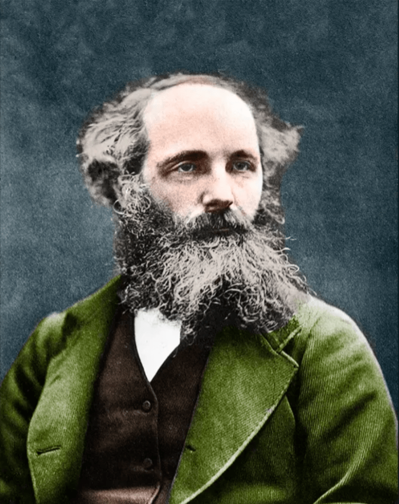
James Clerk Maxwell
James Clerk Maxwell (1831 – 1879) was one of three titans out of Cambridge who served as the intellectual leaders in mid-nineteenth-century Britain. The two others were George Stokes and William Thomson (Lord Kelvin). All three were Wranglers, the top finishers on the Tripos exam at Cambridge, the grueling eight-day examination across all fields of mathematics. The winner of the Tripos, known as first Wrangler, was announced with great fanfare in the local papers, and the lucky student was acclaimed like a sports hero is today. Stokes in 1841 was first Wrangler while Thomson (Lord Kelvin) in 1845 and Maxwell in 1854 were each second Wranglers. They were also each winners of the Smith’s Prize, the top examination at Cambridge for mathematical originality. When Maxwell sat for the Smith’s Prize in 1854 one of the exam problems was a proof written by Stokes on a suggestion by Thomson. Maxwell failed to achieve the proof, though he did win the Prize. The problem became known as Stokes’ Theorem, one of the fundamental theorems of vector calculus, and the proof was eventually provided by Hermann Hankel in 1861.
After graduation from Cambridge, Maxwell took the chair of natural philosophy at Marischal College in the city of Aberdeen in Scotland. He was only 25 years old when he began, fifteen years younger than any of the other professors. He split his time between the university and his family home at Glenlair in the south of Scotland, which he inherited from his father the same year he began his chair at Aberdeen. His research interests spanned from the perception of color to the rings of Saturn. He improved on Thomas Young’s three-color theory by correctly identifying red, green and blue as the primary receptors of the eye and invented a scheme for adding colors that is close to the HSV (hue-saturation-value) system used today in computer graphics. In his work on the rings of Saturn, he developed a statistical mechanical approach to explain how the large-scale structure emerged from the interactions among the small grains. He applied these same techniques several years later to the problem of ideal gases when he derived the speed distribution known today as the Maxwell-Boltzmann distribution.
Maxwell’s career at Aberdeen held great promise until he was suddenly fired from his post in 1860 when Marischal College merged with nearby King’s College to form the University of Aberdeen. After the merger, the university had the abundance of two professors of Natural Philosophy while needing only one, and Maxwell was the junior. With his new wife, Maxwell retired to Glenlair and buried himself in writing the first drafts of a paper titled “On Physical Lines of Force” [2]. The paper explored the mathematical and mechanical aspects of the curious lines of magnetic force that Michael Faraday had first proposed in 1831 and which Thomson had developed mathematically around 1845 as the first field theory in physics.
As Maxwell explored the interrelationships among electric and magnetic phenomena, he derived a wave equation for the electric and magnetic fields and was astounded to find that the speed of electromagnetic waves was essentially the same as the speed of light. The importance of this coincidence did not escape him, and he concluded that light—that rarified, enigmatic and quintessential fifth element—must be electromagnetic in origin. Ever since Francois Arago and Agustin Fresnel had shown that light was a wave phenomenon, scientists had been searching for other physical signs of the medium that supported the waves—a medium known as the luminiferous aether (or ether). With Maxwell’s new finding, it meant that the luminiferous ether must be related to electric and magnetic fields. In the Steampunk tradition of his day, Maxwell began a search for a mechanical model. He did not need to look far, because his friend Thomson had already built a theory on a foundation provided by the Irish mathematician James MacCullagh (1809 – 1847)
The Luminiferous Ether
The late 1830’s was a busy time for the luminiferous ether. Agustin-Louis Cauchy published his extensive theory of the ether in 1836, and the self-taught George Green published his highly influential mathematical theory in 1838 which contained many new ideas, such as the emphasis on potentials and his derivation of what came to be called Green’s theorem.
In 1839 MacCullagh took an approach that established a core property of the ether that later inspired both Thomson and Maxwell in their development of electromagnetic field theory. What McCullagh realized was that the energy of the ether could be considered as if it had both kinetic energy and potential energy (ideas and nomenclature that would come several decades later). Most insightful was the fact that the potential energy of the field depended on pure rotation like a vortex. This rotationally elastic ether was a mathematical invention without any mechanical analog, but it successfully described reflection and refraction as well as polarization of light in crystalline optics.
In 1856 Thomson put Faraday’s famous magneto-optic rotation of light (the Faraday Effect discovered by Faraday in 1845) into mathematical form and began putting Faraday’s initially abstract ideas of the theory of fields into concrete equations. He drew from MacCullagh’s rotational ether as well as an idea from William Rankine about the molecular vortex model of atoms to develop a mechanical vortex model of the ether. Thomson explained how the magnetic field rotated the linear polarization of light through the action of a multiplicity of molecular vortices. Inspired by Thomson, Maxwell took up the idea of molecular vortices as well as Faraday’s magnetic induction in free space and transferred the vortices from being a property exclusively of matter to being a property of the luminiferous ether that supported the electric and magnetic fields.
Maxwellian Cogwheels
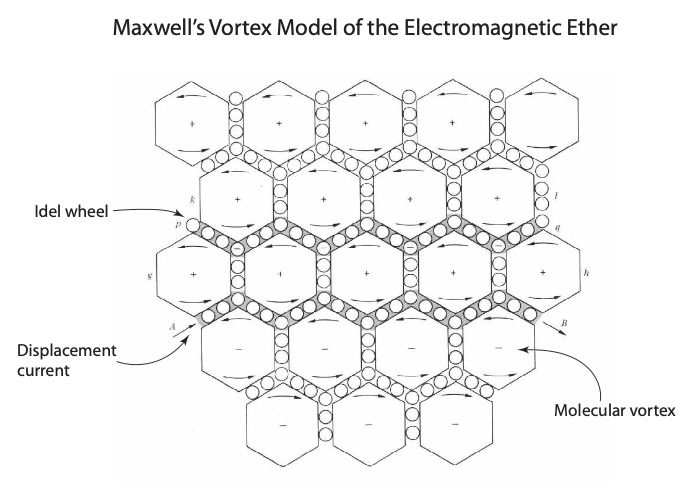
Maxwell’s model of the electromagnetic fields in the ether is the apex of Victorian mechanistic philosophy—too explicit to be a true model of reality—yet it was amazingly fruitful as a tool of discovery, helping Maxwell develop his theory of electrodynamics. The model consisted of an array of elastic vortex cells separated by layers of small particles that acted as “idle wheels” to transfer spin from one vortex to another . The magnetic field was represented by the rotation of the vortices, and the electric current was represented by the displacement of the idle wheels.
Fig. 1 Maxwell’s vortex model of the electromagnetic ether. The molecular vortices rotate according to the direction of the magnetic field, supported by idle wheels. The physical displacement of the idle wheels became an analogy for Maxwell’s displacement current [2].
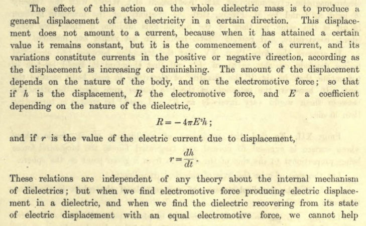
Two predictions by this outrightly mechanical model were to change the physics of electromagnetism forever: First, any change in strain in the electric field would cause the idle wheels to shift, creating a transient current that was called a “displacement current”. This displacement current was one of the last pieces in the electromagnetic puzzle that became Maxwell’s equations.
Fig. 2 In “Physical Lines of Force” in 1861, Maxwell introduces the idea of a displacement current [RefLink].
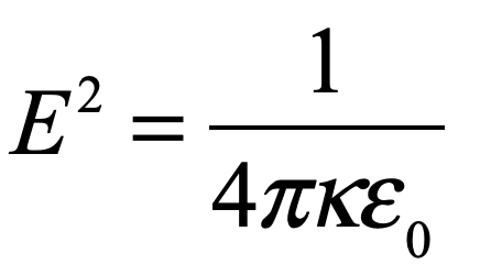
In this description, E is not the electric field, but is related to the dielectric permativity through the relation
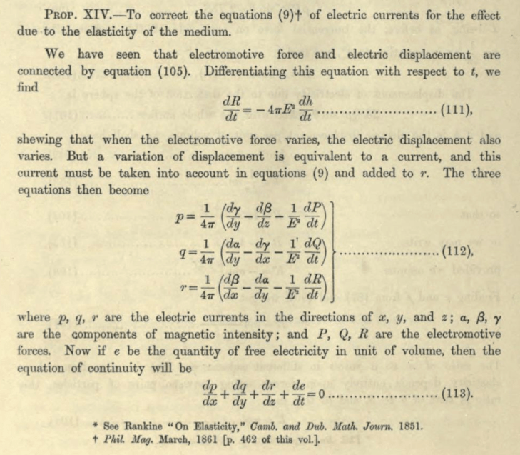
Maxwell went further to prove his Proposition XIV on the contribution of the displacement current to conventional electric currents.
Fig. 3 Maxwell’s Proposition XIV on adding the displacement current to the conventional electric current [RefLink].
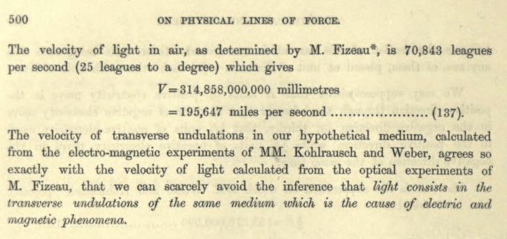
Second, Maxwell calculated that this elastic vortex ether propagated waves at a speed that was close to the known speed of light measured a decade previously by the French physicist Hippolyte Fizeau. He remarked, “we can scarcely avoid the inference that light consists of the transverse undulations of the same medium which is the cause of electric and magnetic phenomena.” [1] This was the first direct prediction that light, previously viewed as a physical process separate from electric and magnetic fields, was an electromagnetic phenomenon.
Fig. 4 Maxwell’s calculation of the speed of light in his mechanical ether. It matched closely the measured speed of light [RefLink].
These two predictions—of the displacement current and the electromagnetic origin of light—have stood the test of time and are center pieces of Maxwells’s legacy. How strange that they arose from a mechanical model of vortices and idle wheels like so many cogs and gears in the machinery powering the Victorian age, yet such is the power of physical visualization.
[1] pg. 12, The Maxwellians, Bruce Hunt (Cornell University Press, 1991)
[2] Maxwell, J. C. (1861). “On physical lines of force”. Philosophical Magazine. 90: 11–23.
At the turn of the New Year, as I turn to the breakthroughs in physics of the previous year, sifting through the candidates, I usually narrow it down to about 4 to 6 that I find personally compelling (See, for instance 2023, 2022). In a given year, they may be related to things like supersolids, condensed atoms, or quantum entanglement. Often they relate to those awful, embarrassing gaps in physics knowledge that we give euphemistic names to, like “Dark Energy” and “Dark Matter” (although in the end they may be neither energy nor matter). But this year, as I sifted, I was struck by how many of the “physics” advances of the past year were focused on pushing limits—lower temperatures, more qubits, larger distances.
If you want something that is eventually useful, then engineering is the way to go, and many of the potential breakthroughs of 2024 did require heroic efforts. But if you are looking for a paradigm shift—a new way of seeing or thinking about our reality—then bigger, better and farther won’t give you that. We may be pushing the boundaries, but the thinking stays the same.
Therefore, for 2024, I have replaced “breakthrough” with a single “prospect” that may force us to change our thinking about the universe and the fundamental forces behind it.
This prospect is the weakening of dark energy over time.
It is a “prospect” because it is not yet absolutely confirmed. If it is confirmed in the next few years, then it changes our view of reality. If it is not confirmed, then it still forces us to think harder about fundamental questions, pointing where to look next.
Einstein’s Cosmological “Constant”
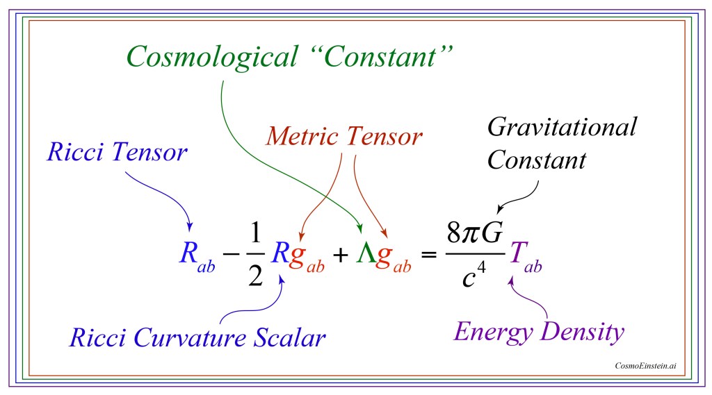
Like so much of physics today, the origins of this story go back to Einstein. At the height of WWI in 1917, as Einstein was working in Berlin, he “tweaked” his new theory of general relativity to allow the universe to be static. The tweak came in the form of a parameter he labelled Lambda (Λ), providing a counterbalance against the gravitational collapse of the universe, which at the time was assumed to have a time-invariant density. This cosmological “constant” of spacetime represented a pressure that kept the universe inflated like a balloon.
Fig. 1 Einstein’s “Field Equations” for the universe containing expressions for curvature, the metric tensor and energy density. Spacetime is warped by energy density, and trajectories within the warped spacetime follow geodesic curves. When Λ = 0, only gravitional attraction is present. When Λ ≠ 0, a “repulsive” background force exerts a pressure on spacetime, keeping it inflated like a balloon.
Later, in 1929 when Edwin Hubble discovered that the universe was not static but was expanding, and not only expanding, but apparently on a free trajectory originating at some point in the past (the Big Bang), Einstein zeroed out his cosmological constant, viewing it as one of his greatest blunders.
And so it stood until 1998 when two teams announced that the expansion of the universe is accelerating—and Einstein’s cosmological constant was back in. In addition, measurements of the energy density of the universe showed that the cosmological constant was contributing around 68% of the total energy density, which has been given the name of Dark Energy. One of the ways to measure Dark Energy is through BAO.
Baryon Acoustic Oscillations (BAO)
If the goal of science communication is to be transparent, and to engage the public in the heroic pursuit of pure science, then the moniker Baryon Acoustic Oscillations (BAO) was perhaps the wrong turn of phrase. “Cosmic Ripples” might have been a better analogy (and a bit more poetic).
In the early moments after the Big Bang, slight density fluctuations set up a balance of opposing effects between gravitational attraction, that tends to clump matter, and the homogenization effects of the hot photon background, that tends to disperse ionized matter. Matter consists of both dark matter as well as the matter we are composed of, known as baryonic matter. Only baryonic matter can be ionized and hence interact with photons, hence only photons and baryons experience this balance. As the universe expanded, an initial clump of baryons and photons expanded outward together, like the ripples on a millpond caused by a thrown pebble. And because the early universe had many clumps (and anti-clumps where density was lower than average), the millpond ripples were like those from a gentle rain with many expanding ringlets overlapping.
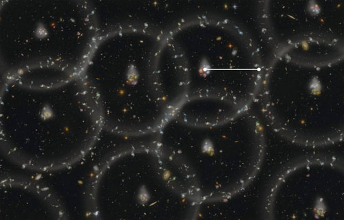
Fig. 2 Overlapping ripples showing galaxies formed along the shells. The size of the shells is set by the speed of “sound” in the universe. From [Ref].
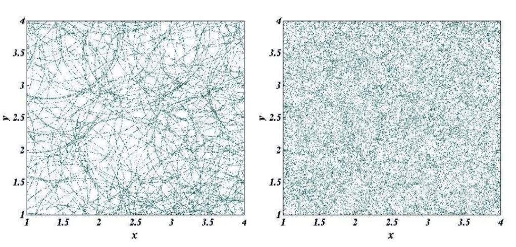
Fig. 3 Left. Galaxies formed on acoustic ringlets like drops of dew on a spider’s web. Right. Many ringlets overlapping. The characteristic size of the ringlets can still be extracted statistically. From [Ref].
Then, about 400,000 years after the Big Bang, as the universe expanded and cooled, it got cold enough that ionized electrons and baryons formed atoms that are neutral and transparent to light. Light suddenly flew free, decoupled from the matter that had constrained it. Removing the balance between light and matter in the BAO caused the baryonic ripples to freeze in place, as if a sudden arctic blast froze the millpond in an instant. The residual clumps of matter in the early universe became clumps of galaxies in the modern universe that we can see and measure. We can also see the effects of those clumps on the temperature fluctuations of the cosmic microwave background (CMB).
Between these two—the BAO and the CMB—it is possible to measure cosmic distances, and with those distances, to measure how fast the universe is expanding.
Acceleration Slowing
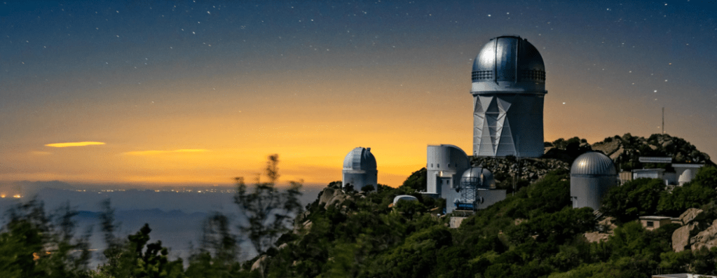
The Dark Energy Spectroscopic Instrument (DESI) on top of Kitt Peak in Arizona is measuring the distances to millions of galaxies using automated fiber optic arrays containing thousands of optical fibers. In one year it measured the distances to about 6 milliion galaxies.
Fig. 4 The Kitt Peak observatory, the site of DESI. From [Ref].
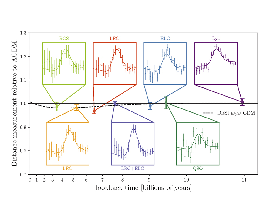
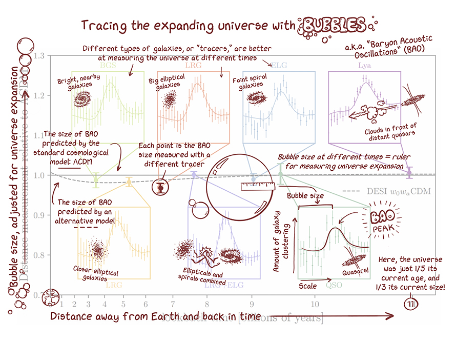
By focusing on seven “epochs” in galaxy formation in the universe, it measures the sizes of the BAO ripples over time, ranging in ages from 3 billion to 11 billion years ago. (The universe is about 13.8 billion years old.) The relative sizes are then compared to the predictions of the LCDM (Lambda-Cold-Dark-Matter) model. This is the “consensus” model of the day—agreed upon as being “most likely” to explain observations. If Dark Energy is a true constant, then the relative sizes of the ripples should all be the same, regardless of how far back in time we look.
But what the DESI data discovered is that relative sizes more recently (a few billion years ago) are smaller than predicted by LCDM. Given that LCDM includes the acceleration of the expansion of the universe caused by Dark Energy, it means that Dark Energy is slightly weaker in the past few billion years than it was 10 billion years ago—it’s weakening or “thawing”.
The measurements as they stand today are shown in Fig. 5, showing the relative sizes as a function of how far back in time they look, with a dashed line showing the deviation from the LCDM prediction. The error bars in the figure are not yet are that impressive, and statistical effects may be causing the trend, so it might be erased by more measurements. But the BAO results have been augmented by recent measurements of supernova (SNe) that provide additional support for thawing Dark Energy. Combined, the BAO+SNe results currently stand at about 3.4 sigma. The gold standard for “discovery” is about 5 sigma, so there is still room for this effect to disappear. So stay tuned—the final answer may be known within a few years.
Fig. 5 Seven “epochs” in the evolution of galaxies in the universe. This plot shows relative galactic distances as a function of time looking back towards the Big Bang (older times closer to the Big Bang are to the right side of the graph). In more recent times, relative distances are smaller than predicted by the consensus theory known as Lambda-Cold-Dark-Matter (LCDM), suggesting that Dark Energy is slight weaker today than it was billions of years ago. The three left-most data points (with error bars from early 2024) are below the LCDM line. From [Ref].Fig. 6 Annotated version of the previous figure. From [Ref].
The Future of Physics
The gravitational constant G is considered to be a constant property of nature, as is Planck’s constant h, and the charge of the electron e. None of these fundamental properties of physics are viewed as time dependent and none can be derived from basic principles. They are simply constants of our reality. But if Λ is time dependent, then it is not a fundamental constant and should be derivable and explainable.
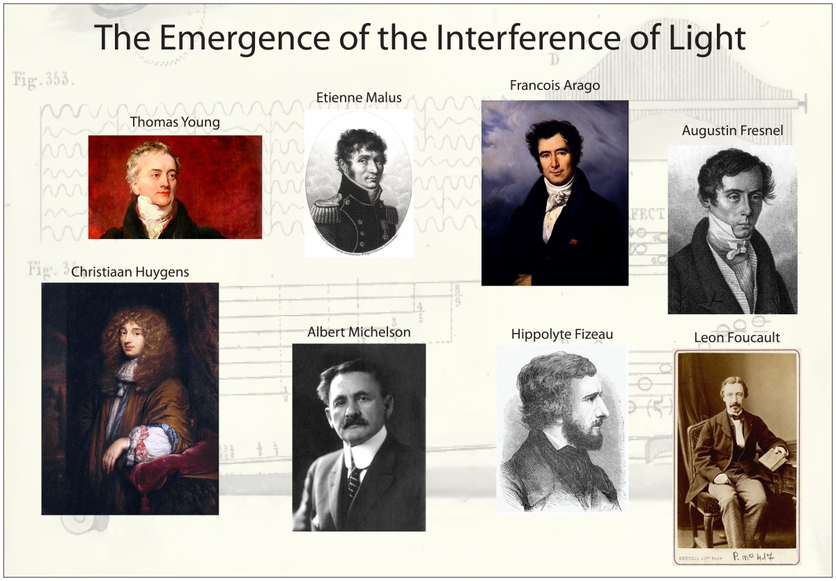
Light is one of the most powerful manifestations of the forces of physics because it tells us about our reality. The interference of light, in particular, has led to the detection of exoplanets orbiting distant stars, discovery of the first gravitational waves, capture of images of black holes and much more. The stories behind the history of light and interference go to the heart of how scientists do what they do and what they often have to overcome to do it. These time-lines are organized along the chapter titles of the book Interference. They follow the path of theories of light from the first wave-particle debate, through the personal firestorms of Albert Michelson, to the discoveries of the present day in quantum information sciences.
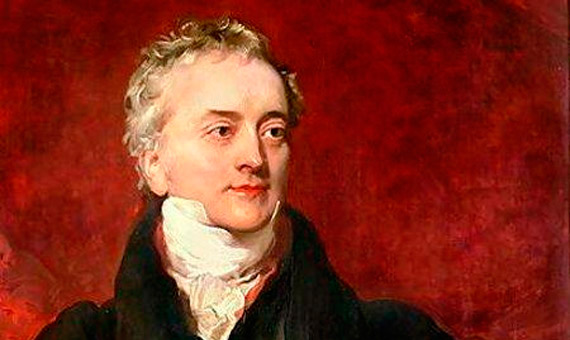
Thomas Young was the ultimate dabbler, his interests and explorations ranged far and wide, from ancient egyptology to naval engineering, from physiology of perception to the physics of sound and light. Yet unlike most dabblers who accomplish little, he made original and seminal contributions to all these fields. Some have called him the “Last Man Who Knew Everything“.
Thomas Young. The Law of Interference.
Topics: The Law of Interference. The Rosetta Stone. Benjamin Thompson, Count Rumford. Royal Society. Christiaan Huygens. Pendulum Clocks. Icelandic Spar. Huygens’ Principle. Stellar Aberration. Speed of Light. Double-slit Experiment.
1629 – Huygens born (1629 – 1695)
1642 – Galileo dies, Newton born (1642 – 1727)
1655 – Huygens ring of Saturn
1657 – Huygens patents the pendulum clock
1666 – Newton prismatic colors
1666 – Huygens moves to Paris
1669 – Bartholin double refraction in Icelandic spar
1670 – Bartholinus polarization of light by crystals
1671 – Expedition to Hven by Picard and Rømer
1673 – James Gregory bird-feather diffraction grating
1801 – Young Theory of Light and Colours, three color mechanism (Bakerian Lecture), Young considers interference to cause the colored films, first estimates of the wavelengths of different colors
1802 – Young begins series of lecturs at the Royal Institution (Jan. 1802 – July 1803)
1802 – Young names the principle (Law) of interference
Augustin Fresnel was an intuitive genius whose talents were almost squandered on his job building roads and bridges in the backwaters of France until he was discovered and rescued by Francois Arago.
Topics: Particles versus Waves. Malus and Polarization. Agustin Fresnel. Francois Arago. Diffraction. Daniel Bernoulli. The Principle of Superposition. Joseph Fourier. Transverse Light Waves.
1665 – Grimaldi diffraction bands outside shadow
1673 – James Gregory bird-feather diffraction grating
There is no question that Francois Arago was a swashbuckler. His life’s story reads like an adventure novel as he went from being marooned in hostile lands early in his career to becoming prime minister of France after the 1848 revolutions swept across Europe.
Topics: The Birth of Interferometry. Snell’s Law. Fresnel and Arago. The First Interferometer. Fizeau and Foucault. The Speed of Light. Ether Drag. Jamin Interferometer.
No name is more closely connected to interferometry than that of Albert Michelson. He succeeded, sometimes at great personal cost, in launching interferometric metrology as one of the most important tools used by scientists today.
Albert A. Michelson, 1907 Nobel Prize. Image Credit.
Topics: The Trials of Albert Michelson. Hermann von Helmholtz. Michelson and Morley. Fabry and Perot.
1810 – Arago search for ether drag
1813 – Fraunhofer dark lines in Sun spectrum
1813 – Faraday begins at Royal Institution
1820 – Oersted discovers electromagnetism
1821 – Faraday electromagnetic phenomena
1827 – Green mathematical analysis of electricity and magnetism
1830 – Cauchy ether as elastic solid
1831 – Faraday electromagnetic induction
1831 – Cauchy ether drag
1831 – Maxwell born
1831 – Faraday electromagnetic induction
1836 – Cauchy’s second theory of the ether
1838 – Green theory of the ether
1839 – Hamilton group velocity
1839 – MacCullagh properties of rotational ether
1839 – Cauchy ether with negative compressibility
1841 – Maxwell entered Edinburgh Academy (age 10) met P. G. Tait
1842 – Doppler effect
1845 – Faraday effect (magneto-optic rotation)
1846 – Stokes’ viscoelastic theory of the ether
1847 – Maxwell entered Edinburgh University
1850 – Maxwell at Cambridge, studied under Hopkins, also knew Stokes and Whewell
1852 – Michelson born Strelno, Prussia
1854 – Maxwell wins the Smith’s Prize (Stokes’ theorem was one of the problems)
1855 – Michelson’s immigrate to San Francisco through Panama Canal
Learning from his attempts to measure the speed of light through the ether, Michelson realized that the partial coherence of light from astronomical sources could be used to measure their sizes. His first measurements using the Michelson Stellar Interferometer launched a major subfield of astronomy that is one of the most active today.
R Hanbury Brown
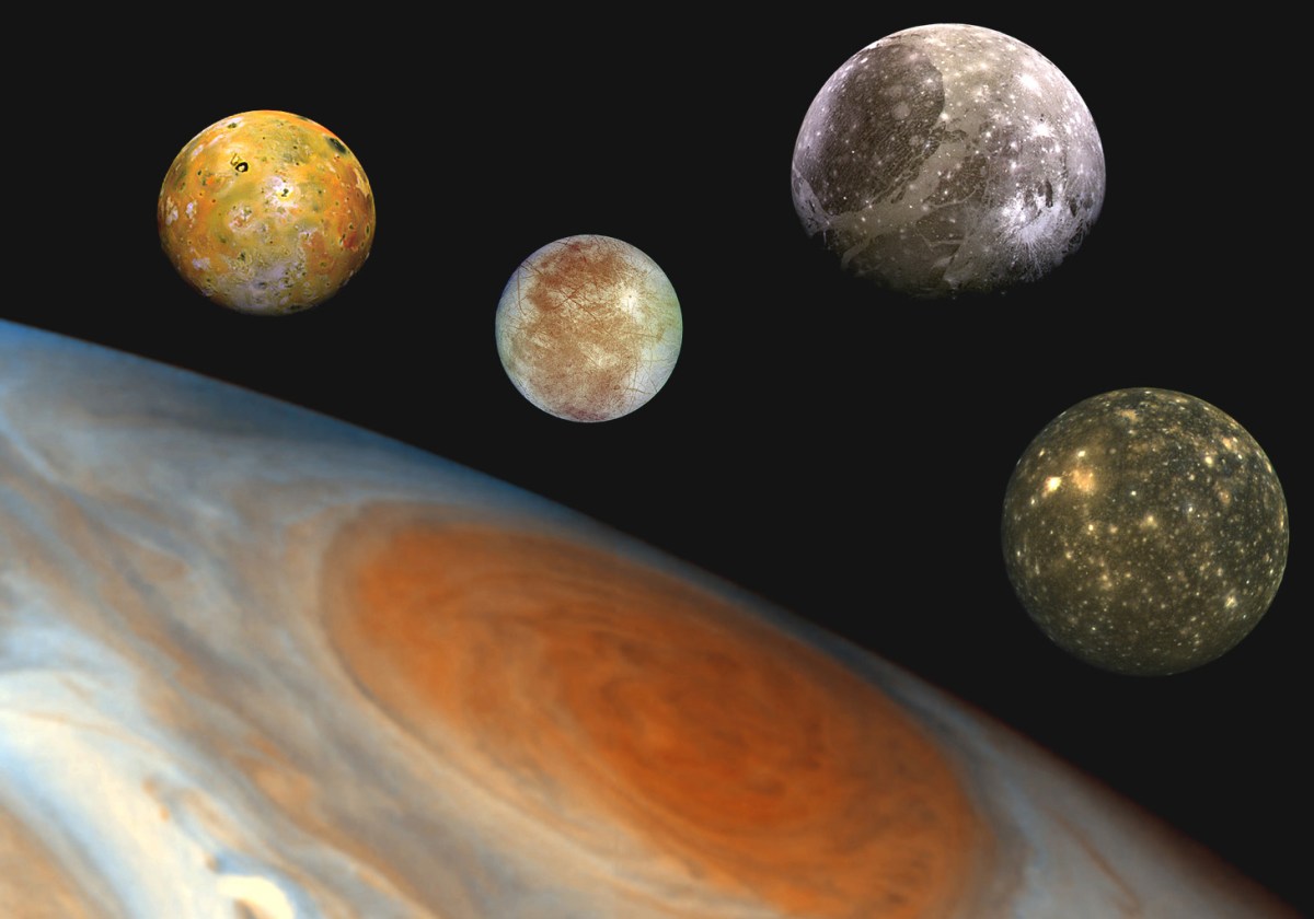
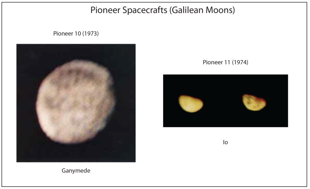
Topics: Measuring the Stars. Astrometry. Moons of Jupiter. Schwarzschild. Betelgeuse. Michelson Stellar Interferometer. Banbury Brown Twiss. Sirius. Adaptive Optics.
1838 – Bessel stellar parallax measurement with Fraunhofer telescope
1868 – Fizeau proposes stellar interferometry
1873 – Stephan implements Fizeau’s stellar interferometer on Sirius, sees fringes
1880 – Michelson Idea for second-order measurement of relative motion against ether
1880 – 1882 Michelson Studies in Europe (Helmholtz in Berlin, Quincke in Heidelberg, Cornu, Mascart and Lippman in Paris)
1881 – Michelson Measurement at Potsdam with funds from Alexander Graham Bell
1881 – Michelson Resigned from active duty in the Navy
1883 – Michelson Joined Case School of Applied Science
1889 – Michelson moved to Clark University at Worcester
Stellar interferometry is opening new vistas of astronomy, exploring the wildest occupants of our universe, from colliding black holes half-way across the universe (LIGO) to images of neighboring black holes (EHT) to exoplanets near Earth that may harbor life.
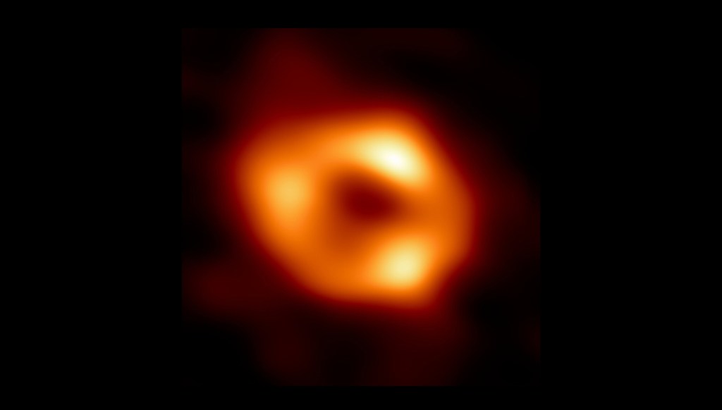
Image of the supermassive black hole in M87 from Event Horizon Telescope.
Topics: Gravitational Waves, Black Holes and the Search for Exoplanets. Nulling Interferometer. Event Horizon Telescope. M87 Black Hole. Long Baseline Interferometry. LIGO.
1947 – Virgo A radio source identified as M87
1953 – Horace W. Babcock proposes adaptive optics (AO)
From the astronomically large dimensions of outer space to the microscopically small dimensions of inner space, optical interference pushes the resolution limits of imaging.
Topics: Diffraction and Interference. Joseph Fraunhofer. Diffraction Gratings. Henry Rowland. Carl Zeiss. Ernst Abbe. Phase-contrast Microscopy. Super-resolution Micrscopes. Structured Illumination.
The coherence of laser light is like a brilliant jewel that sparkles in the darkness, illuminating life, probing science and projecting holograms in virtual worlds.
What is the image of one photon interfering? Better yet, what is the image of two photons interfering? The answer to this crucial question laid the foundation for quantum communication.
Topics: The Beginnings of Quantum Communication. EPR paradox. Entanglement. David Bohm. John Bell. The Bell Inequalities. Leonard Mandel. Single-photon Interferometry. HOM Interferometer. Two-photon Fringes. Quantum cryptography. Quantum Teleportation.
1900 – Planck (1901). “Law of energy distribution in normal spectra.” [1]
There is almost no technical advantage better than having exponential resources at hand. The exponential resources of quantum interference provide that advantage to quantum computing which is poised to usher in a new era of quantum information science and technology.
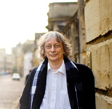
David Deutsch.
Topics: Interferometric Computing. David Deutsch. Quantum Algorithm. Peter Shor. Prime Factorization. Quantum Logic Gates. Linear Optical Quantum Computing. Boson Sampling. Quantum Computational Advantage.
1980 – Paul Benioff describes possibility of quantum computer
[10] B. R. Mollow, R. J. Glauber: Phys. Rev. 160, 1097 (1967); 162, 1256 (1967)
[11] J. F. Clauser, M. A. Horne, A. Shimony, and R. A. Holt, ” Proposed experiment to test local hidden-variable theories,” Physical Review Letters, vol. 23, no. 15, pp. 880-&, (1969)
[15] R. Ghosh and L. Mandel, “Observation of nonclassical effects in the interference of 2 photons,” Physical Review Letters, vol. 59, no. 17, pp. 1903-1905, Oct (1987)
[16] C. K. Hong, Z. Y. Ou, and L. Mandel, “Measurement of subpicosecond time intervals between 2 photons by interference,” Physical Review Letters, vol. 59, no. 18, pp. 2044-2046, Nov (1987)
[18] D. Deutsch, “QUANTUM-THEORY, THE CHURCH-TURING PRINCIPLE AND THE UNIVERSAL QUANTUM COMPUTER,” Proceedings of the Royal Society of London Series a-Mathematical Physical and Engineering Sciences, vol. 400, no. 1818, pp. 97-117, (1985)
[19] P. W. Shor, “ALGORITHMS FOR QUANTUM COMPUTATION – DISCRETE LOGARITHMS AND FACTORING,” in 35th Annual Symposium on Foundations of Computer Science, Proceedings, S. Goldwasser Ed., (Annual Symposium on Foundations of Computer Science, 1994, pp. 124-134.
[20] F. Arute et al., “Quantum supremacy using a programmable superconducting processor,” Nature, vol. 574, no. 7779, pp. 505-+, Oct 24 (2019)
[21] H.-S. Zhong et al., “Quantum computational advantage using photons,” Science, vol. 370, no. 6523, p. 1460, (2020)
Further Reading: The History of Light and Interference (2023)
The first step on the road to Einstein’s relativity was taken a hundred years earlier by an ironic rebel of physics—Augustin Fresnel. His radical (at the time) wave theory of light was so successful, especially the proof that it must be composed of transverse waves, that he was single-handedly responsible for creating the irksome luminiferous aether that would haunt physicists for the next century. It was only when Einstein combined the work of Fresnel with that of Hippolyte Fizeau that the aether was ultimately banished.
Augustin Fresnel: Ironic Rebel of Physics
Augustin Fresnel was an odd genius who struggled to find his place in the technical hierarchies of France. After graduating from the Ecole Polytechnique, Fresnel was assigned a mindless job overseeing the building of roads and bridges in the boondocks of France—work he hated. To keep himself from going mad, he toyed with physics in his spare time, and he stumbled on inconsistencies in Newton’s particulate theory of light that Laplace, a leader of the French scientific community, embraced as if it were revealed truth .
The final irony is that Einstein used Fresnel’s theoretical coefficient and Fizeau’s measurements—that had introduced aether drag in the first place—to show that there was no aether.
Fresnel rebelled, realizing that effects of diffraction could be explained if light were made of waves. He wrote up an initial outline of his new wave theory of light, but he could get no one to listen, until Francois Arago heard of it. Arago was having his own doubts about the particle theory of light based on his experiments on stellar aberration.
Augustin Fresnel and Francois Arago (circa 1818)
Stellar Aberration and the Fresnel Drag Coefficient
Stellar aberration had been explained by James Bradley in 1729 as the effect of the motion of the Earth relative to the motion of light “particles” coming from a star. The Earth’s motion made it look like the star was tilted at a very small angle (see my previous blog). That explanation had worked fine for nearly a hundred years, but then around 1810 Francois Arago at the Paris Observatory made extremely precise measurements of stellar aberration while placing finely ground glass prisms in front of his telescope. According to Snell’s law of refraction, which depended on the velocity of the light particles, the refraction angle should have been different at different times of the year when the Earth was moving one way or another relative to the speed of the light particles. But to high precision the effect was absent. Arago began to question the particle theory of light. When he heard about Fresnel’s work on the wave theory, he arranged a meeting, encouraging Fresnel to continue his work.
But at just this moment, in March of 1815, Napoleon returned from exile in Elba and began his march on Paris with a swelling army of soldiers who flocked to him. Fresnel rebelled again, joining a royalist militia to oppose Napoleon’s return. Napoleon won, but so did Fresnel, who was ironically placed under house arrest, which was like heaven to him. It freed him from building roads and bridges, giving him free time to do optics experiments in his mother’s house to support his growing theoretical work on the wave nature of light.
Arago convinced the authorities to allow Fresnel to come to Paris, where the two began experiments on diffraction and interference. By using polarizers to control the polarization of the interfering light paths, they concluded that light must be composed of transverse waves.
This brilliant insight was then followed by one of the great tragedies of science—waves needed a medium within which to propagate, so Fresnel conceived of the luminiferous aether to support it. Worse, the transverse properties of light required the aether to have a form of crystalline stiffness.
How could moving objects, like the Earth orbiting the sun, travel through such an aether without resistance? This was a serious problem for physics. One solution was that the aether was entrained by matter, so that as matter moved, the aether was dragged along with it. That solved the resistance problem, but it raised others, because it couldn’t explain Arago’s refraction measurements of aberration.
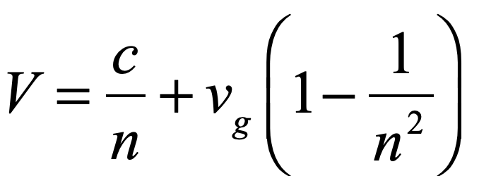
Fresnel realized that Arago’s null results could be explained if aether was only partially dragged along by matter. For instance, in the glass prisms used by Arago, the fraction of the aether being dragged along by the moving glass versus at rest would depend on the refractive index n of the glass. The speed of light in moving glass would then be
where c is the speed of light through stationary aether, vg is the speed of the glass prism through the stationary aether, and V is the speed of light in the moving glass. The first term in the expression is the ordinary definition of the speed of light in stationary matter with the refractive index. The second term is called the Fresnel drag coefficient which he communicated to Arago in a letter in 1818. Even at the high speed of the Earth moving around the sun, this second term is a correction of only about one part in ten thousand. It explained Arago’s null results for stellar aberration, but it was not possible to measure it directly in the laboratory at that time.
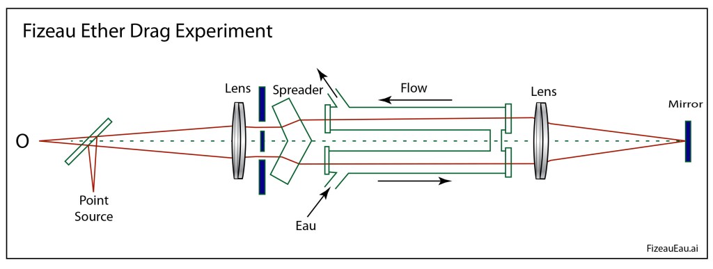
Fizeau’s Moving Water Experiment
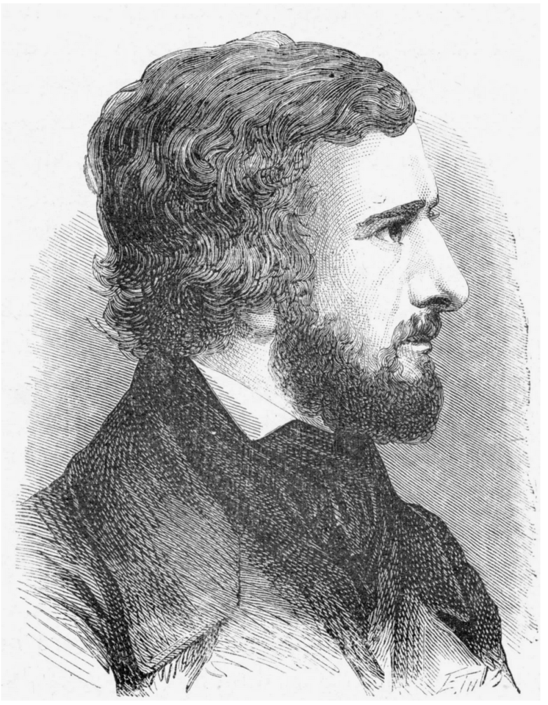
Hippolyte Fizeau has the distinction of being the first to measure the speed of light directly in an Earth-bound experiment. All previous measurements had been astronomical. The story of his ingenious use of a chopper wheel and long-distance reflecting mirrors placed across the city of Paris in 1849 can be found in Chapter 3 of Interference. However, two years later he completed an experiment that few at the time noticed but which had a much more profound impact on the history of physics.
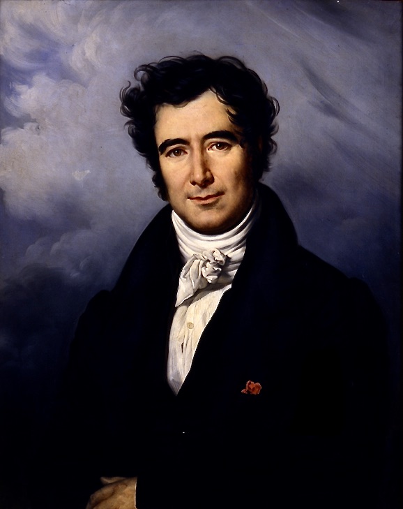
Hippolyte Fizeau
In 1851, Fizeau modified an Arago interferometer to pass two interfering light beams along pipes of moving water. The goal of the experiment was to measure the aether drag coefficient directly and to test Fresnel’s theory of partial aether drag. The interferometer allowed Fizeau to measure the speed of light in moving water relative to the speed of light in stationary water. The results of the experiment confirmed Fresnel’s drag coefficient to high accuracy, which seemed to confirm the partial drag of aether by moving matter.
Fizeau’s 1851 measurement of the speed of light in water using a modified Arago interferometer. (Reprinted from Chapter 2: Interference.)
This result stood for thirty years, presenting its own challenges for physicist exploring theories of the aether. The sophistication of interferometry improved over that time, and in 1881 Albert Michelson used his newly-invented interferometer to measure the speed of the Earth through the aether. He performed the experiment in the Potsdam Observatory outside Berlin, Germany, and found the opposite result of complete aether drag, contradicting Fizeau’s experiment. Later, after he began collaborating with Edwin Morley at Case and Western Reserve Colleges in Cleveland, Ohio, the two repeated Fizeau’s experiment to even better precision, finding once again Fresnel’s drag coefficient, followed by their own experiment, known now as “the Michelson-Morley Experiment” in 1887, that found no effect of the Earth’s movement through the aether.
The two experiments—Fizeau’s measurement of the Fresnel drag coefficient, and Michelson’s null measurement of the Earth’s motion—were in direct contradiction with each other. Based on the theory of the aether, they could not both be true.
But where to go from there? For the next 15 years, there were numerous attempts to put bandages on the aether theory, from Fitzgerald’s contraction to Lorenz’ transformations, but it all seemed like kludges built on top of kludges. None of it was elegant—until Einstein had his crucial insight.
Einstein’s Insight
While all the other top physicists at the time were trying to save the aether, taking its real existence as a fact of Nature to be reconciled with experiment, Einstein took the opposite approach—he assumed that the aether did not exist and began looking for what the experimental consequences would be.
From the days of Galileo, it was known that measured speeds depended on the frame of reference. This is why a knife dropped by a sailor climbing the mast of a moving ship strikes at the base of the mast, falling in a straight line in the sailor’s frame of reference, but an observer on the shore sees the knife making an arc—velocities of relative motion must add. But physicists had over-generalized this result and tried to apply it to light—Arago, Fresnel, Fizeau, Michelson, Lorenz—they were all locked in a mindset.
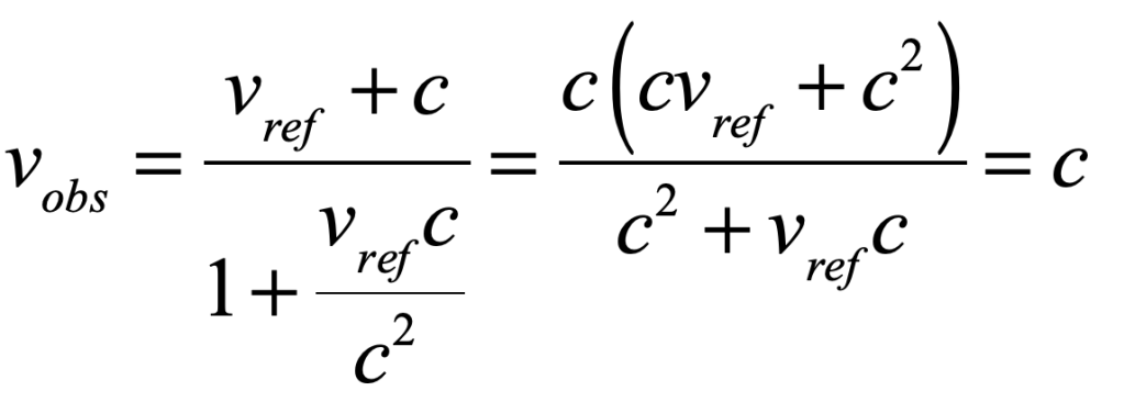
Einstein stepped outside that mindset and asked what would happen if all relatively moving observers measured the same value for the speed of light, regardless of their relative motion. It was just a little algebra to find that the way to add the speed of light c to the speed of a moving reference frame vref was
where the numerator was the usual Galilean relativity velocity addition, and the denominator was required to enforce the constancy of observed light speeds. Therefore, adding the speed of light to the speed of a moving reference frame gives back simply the speed of light.
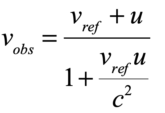
Generalizing this equation for general velocity addition between moving frames gives
where u is now the speed of some moving object being added the the speed of a reference frame, and vobs is the “net” speed observed by some “external” observer . This is Einstein’s famous equation for relativistic velocity addition (see pg. 12 of the English translation). It ensures that all observers with differently moving frames all measure the same speed of light, while also predicting that no velocities for objects can ever exceed the speed of light.
This last fact is a consequence, not an assumption, as can be seen by letting the reference speed vref increase towards the speed of light so that vref ≈ c, then
so that the speed of an object launched in the forward direction from a reference frame moving near the speed of light is still observed to be no faster than the speed of light
All of this, so far, is theoretical. Einstein then looked to find some experimental verification of his new theory of relativistic velocity addition, and he thought of the Fizeau experimental measurement of the speed of light in moving water. Applying his new velocity addition formula to the Fizeau experiment, he set vref = vwater and u = c/n and found
The second term in the denominator is much smaller that unity and is expanded in a Taylor’s expansion
The last line is exactly the Fresnel drag coefficient!
Therefore, Fizeau, half a century before, in 1851, had already provided experimental verification of Einstein’s new theory for relativistic velocity addition! It wasn’t aether drag at all—it was relativistic velocity addition.
From this point onward, Einstein followed consequence after inexorable consequence, constructing what is now called his theory of Special Relativity, complete with relativistic transformations of time and space and energy and matter—all following from a simple postulate of the constancy of the speed of light and the prescription for the addition of velocities.
The final irony is that Einstein used Fresnel’s theoretical coefficient and Fizeau’s measurements, that had established aether drag in the first place, as the proof he needed to show that there was no aether. It was all just how you looked at it.
• The history behind Einstein’s use of relativistic velocity addition is given in: A. Pais, Subtle is the Lord: The Science and the Life of Albert Einstein (Oxford University Press, 2005).
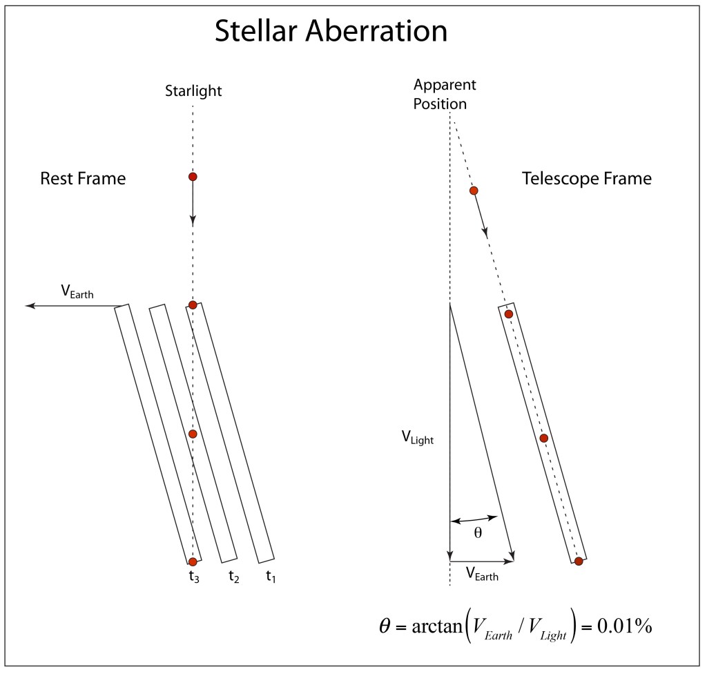
The Earth races around the sun with remarkable speed—at over one hundred thousand kilometers per hour on its yearly track. This is about 0.01% of the speed of light—a small but non-negligible amount for which careful measurement might show the very first evidence of relativistic effects. How big is this effect and how do you measure it? One answer is the aberration of starlight, which is the slight deviation in the apparent position of stars caused by the linear speed of the Earth around the sun.
This is not parallax, which is caused the the changing position of the Earth around the sun. Ever since Copernicus, astronomers had been searching for parallax, which would give some indication how far away stars were. It was an important question, because the answer would say something about how big the universe was. But in the process of looking for parallax, astronomers found something else, something about 50 times bigger—aberration.
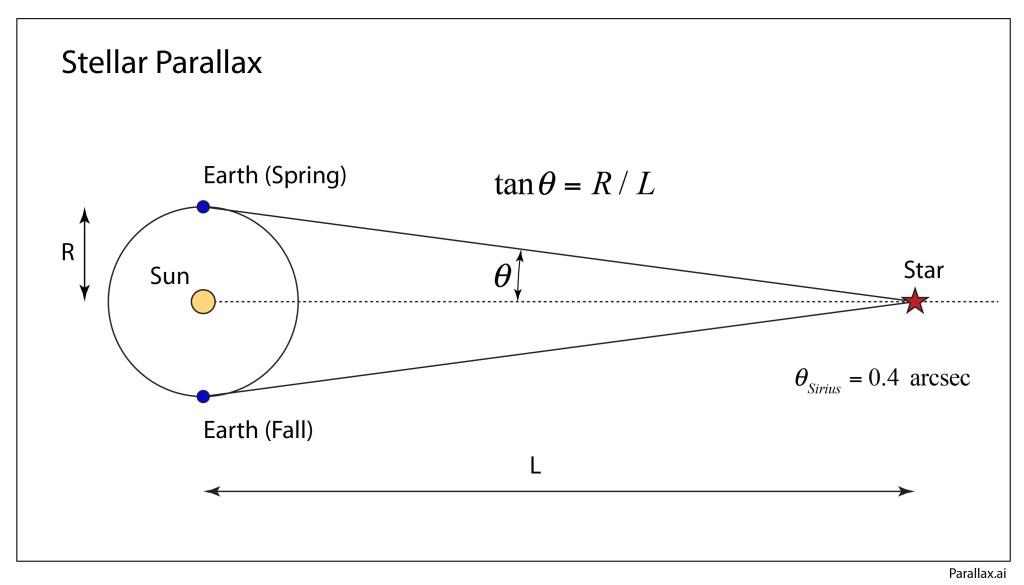
Aberration is the effect of the transverse speed of the Earth added to the speed of light coming from a star. For instance, this effect on the apparent location of stars in the sky is a simple calculation of the arctangent of 0.01%, which is an angle of about 20 seconds of arc, or about 40 seconds when comparing two angles 6 months apart. This was a bit bigger than the accuracy of astronomical measurements at the time when Jean Picard travelled from Paris to Denmark in 1671 to visit the ruins of the old observatory of Tycho Brahe at Uranibourg.
Fig. 1 Stellar parallax is the change in apparent positions of a star caused by the change in the Earth’s position as it orbits the sun. If the change in angle (θ) could be measured, then based on Newton’s theory of gravitation that gives the radius of the Earth’s orbit (R), the distance to the star (L) could be found.
Jean Picard at Uranibourg
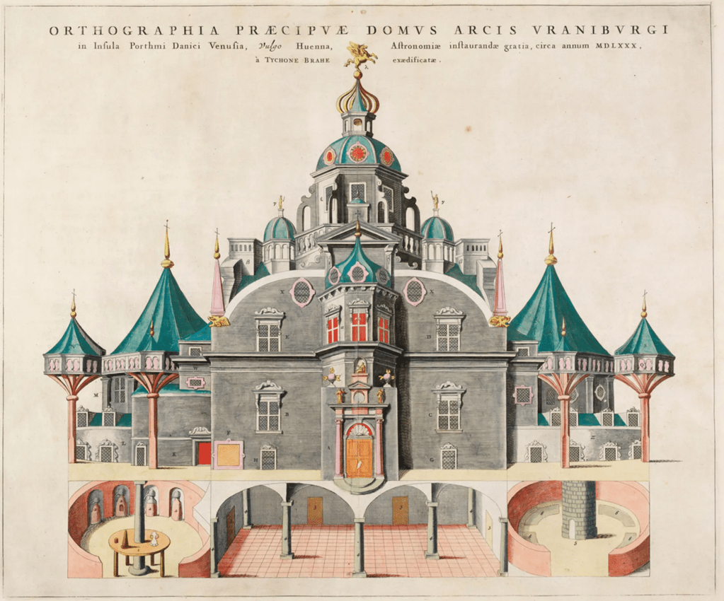
Fig. 2 A view of Tycho Brahe’s Uranibourg astronomical observatory in Hven, Denmark. Tycho had to abandon it near the end of his life when a new king thought he was performing witchcraft.
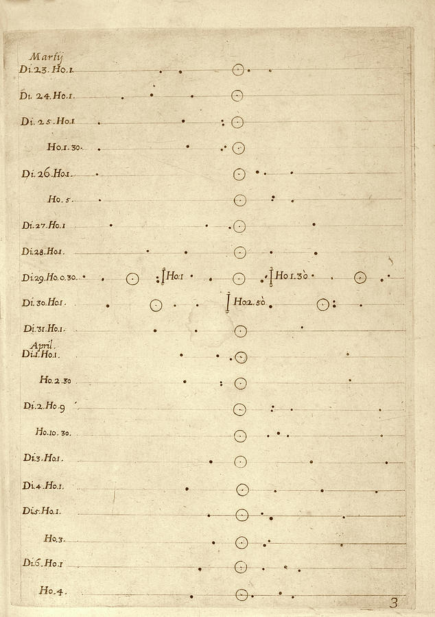
Jean Picard went to Uranibourg originally in 1671, and during subsequent years, to measure the eclipses of the moons of Jupiter to determine longitude at sea—an idea first proposed by Galileo. When visiting Copenhagen, before heading out to the old observatory, Picard secured the services of an as yet unknown astronomer by the name of Ole Rømer. While at Uranibourg, Picard and Rømer made their required measurements of the eclipses of the moons of Jupiter, but with extra observation hours, Picard also made measurements of the positions of selected stars, such as Polaris, the North Star. His very precise measurements allowed him to track a tiny yearly shift, an aberration, in position by about 40 seconds of arc. At the time (before Rømer’s great insight about the finite speed of light—see Chapter 1 of Interference (Oxford, 2023)), the speed of light was thought to be either infinite or unmeasurably fast, so Picard thought that this shift was the long-sought effect of stellar parallax that would serve as a way to measure the distance to the stars. However, the direction of the shift of Polaris was completely wrong if it were caused by parallax, and Picard’s stellar aberration remained a mystery.
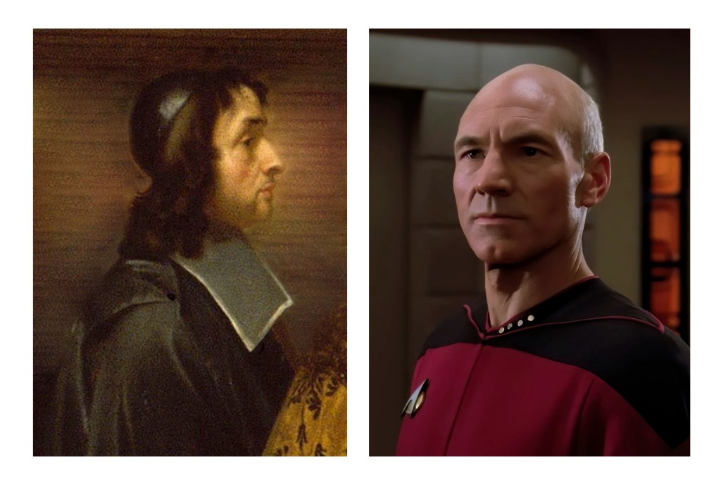
Fig. 3 Jean Picard (left) and his modern name-sake (right).
Samuel Molyneux and Murder in Kew
In 1725, the amateur Irish astronomer Samuel Molyneux (1689 – 1828) decided that the tools of astronomy had improved to the point that the question of parallax could be answered. He enlisted the help of an instrument maker outside London to install a 24-foot zenith sector (a telescope that points vertically upwards) at his home in Kew. Molyneux was an independently wealthy politician (he had married the first daughter of the second Earl of Essex) who sat in the British House of Commons, and he was also secretary to the Prince of Wales (the future George II). Because his political activities made demands on his time, he looked for assistance with his observations and invited James Bradley (1693 – 1762), the newly installed Savilian Professor of Astronomy at Oxford University, to join him in his search.
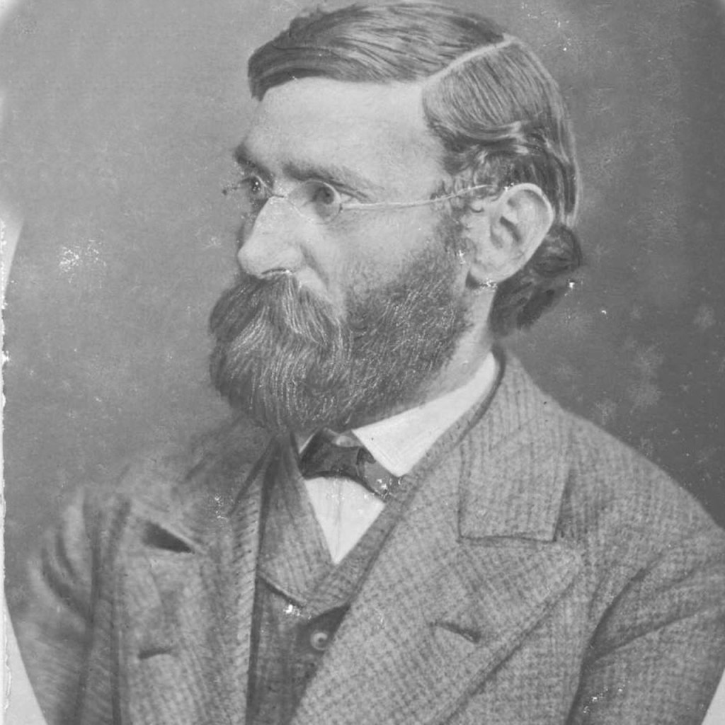
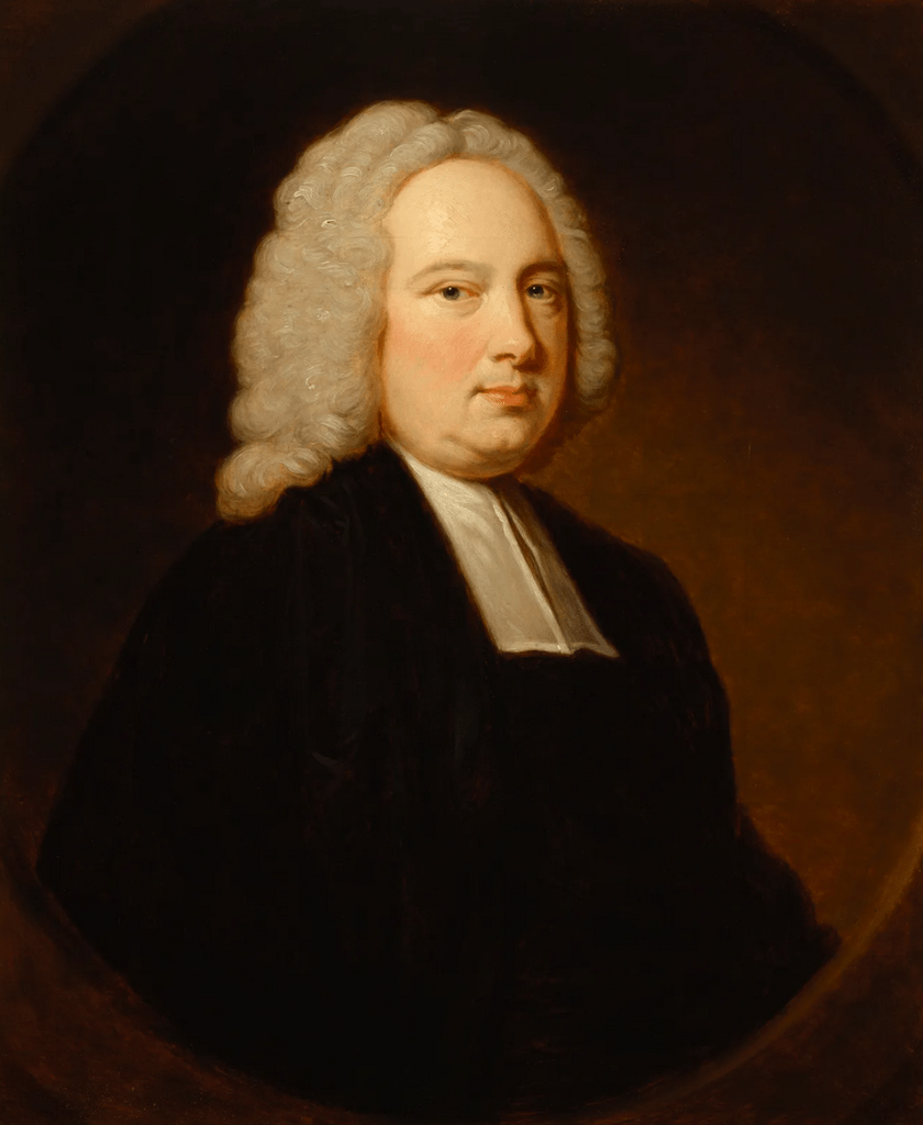
Fig. 4 James Bradley.
James Bradley was a rising star in the scientific circles of England. He came from a modest background but had the good fortune that his mother’s brother, James Pound, was a noted amateur astronomer who had set up a small observatory at his rectory in Wanstead. Bradley showed an early interest in astronomy, and Pound encouraged him, helping with the finances of his education that took him to degrees at Baliol College at Oxford. Even more fortunate was the fact that Pound’s close friend was the Astronomer Royal Edmund Halley, who also took a special interest in Bradley. With Halley’s encouragement, Bradley made important measurements of Mars and several nebulae, demonstrating an ability to work with great accuracy. Halley was impressed and nominated Bradley to the Royal Society in 1718, telling everyone that Bradley was destined to be one of the great astronomers of his time.
Molyneux must have sensed immediately that he had chosen wisely by selecting Bradley to help him with the parallax measurements. Bradley was capable of exceedingly precise work and was fluent mathematically with the geometric complexities of celestial orbits. Fastening the large zenith sector to the chimney of the house gave the apparatus great stability, and in December of 1725 they commenced observations of Gamma Draconis as it passed directly overhead. Because of the accuracy of the sector, they quickly observed a deviation in the star’s position, but the deviation was in the wrong direction, just as Picard had observed. They continued to make observations over two years, obtaining a detailed map of a yearly wobble in the star’s position as it changed angle by 40 seconds of arc (about one percent of a degree) over six months.
When Molyneux was appointed Lord of the Admiralty in 1727, as well as becoming a member of the Irish Parliament (representing Dublin University), he had little time to continue with the observations of Gamma Draconis. He helped Bradley set up a Zenith sector telescope at Bradley’s uncle’s observatory in Wanstead that had a wider field of view to observe more stars, and then he left the project to his friend. A few months later, before either he or Bradley had understood the cause of the stellar aberration, Molyneux collapsed while in the House of Commons and was carried back to his house. One of Molyneux’s many friends was the court anatomist Nathaniel St. André who attended to him over the next several days as he declined and died. St. André was already notorious for roles he had played in several public hoaxes, and on the night of his friend’s death, before the body had grown cold, he eloped with Molyneux’s wife, raising accusations of murder (that could never be proven).
James Bradley and the Light Wind
Over the following year, Bradley observed aberrations in several stars, all of them displaying the same yearly wobble of about 40 seconds of arc. This common behavior of numerous stars demanded a common explanation, something they all shared. It is said that the answer came to Bradley while he was boating on the Thames. The story may be apocryphal, but he apparently noticed the banner fluttering downwind at the top of the mast, and after the boat came about, the banner pointed in a new direction. The wind direction itself had not altered, but the motion of the boat relative to the wind had changed. Light at that time was considered to be made of a flux of corpuscles, like a gentle wind of particles. As the Earth orbited the Sun, its motion relative to this wind would change periodically with the seasons, and the apparent direction of the star would shift a little as a result.
Fig. 5 Principle of stellar aberration. On the left is the rest frame of the star positioned directly overhead as a moving telescope tube must be slightly tilted at an angle (equal to the arctangent of the ratio of the Earth’s speed to the speed of light–greatly exaggerated in the figure) to allow the light to pass through it. On the right is the rest frame of the telescope in which the angular position of the star appears shifted.
Bradley shared his observations and his explanation in a letter to Halley that was read before the Royal Society in January of 1729. Based on his observations, he calculated the speed of light to be about ten thousand times faster than the speed of the Earth in its orbit around the Sun. At that speed, it should take light eight minutes and twelve seconds to travel from the Sun to the Earth (the actual number is eight minutes and 19 seconds). This number was accurate to within a percent of the true value compared with the estimates made by Huygens from the eclipses of the moons of Jupiter that were in error by 27 percent. In addition, because he was unable to discern any effect of parallax in the stellar motions, Bradley was able to place a limit on how far the distant stars must be, more than 100,000 times farther the distance of the Earth from the Sun, which was much farther away than any had previously expected. In January of 1729 the size of the universe suddenly jumped to an incomprehensibly large scale.
Bradley’s explanation of the aberration of starlight was simple and matched observations with good quantitative accuracy. The particle nature of light made it like a wind, or a current, and the motion of the Earth was just a case of Galilean relativity that any freshman physics student can calculate. At first there seemed to be no controversy or difficulties with this interpretation. However, an obscure paper published in 1784 by an obscure English natural philosopher named John Michell (the first person to conceive of a “dark star”) opened a Pandora’s box that launched the crisis of the luminiferous ether and the eventual triumph of Einstein’s theory of Relativity (see Chapter 3 of Interference (Oxford, 2023)), .
By David D. Nolte, Sept. 27, 2023
Read more in Books by David Nolte at Oxford University Press
The constellation Orion strides high across the heavens on cold crisp winter nights in the North, followed at his heel by his constant companion, Canis Major, the Great Dog. Blazing blue from the Dog’s proud chest is the star Sirius, the Dog Star, the brightest star in the night sky. Although it is only the seventh closest star system to our sun, the other six systems host dimmer dwarf stars. Sirius, on the other hand, is a young bright star burning blue in the night. It is an infant star, really, only as old as 5% the age of our sun, coming into being when Dinosaurs walked our planet.
The Sirius star system is a microcosm of mankind’s struggle to understand the Universe. Because it is close and bright, it has become the de facto bench-test for new theories of astrophysics as well as for new astronomical imaging technologies. It has played this role from the earliest days of history, when it was an element of religion rather than of science, down to the modern age as it continues to test and challenge new ideas about quantum matter and extreme physics.
Sirius Through the Ages
To the ancient Egyptians, Sirius was the star Sopdet, the welcome herald of the flooding of the Nile when it rose in the early morning sky of autumn. The star was associated with Isis of the cow constellation Hathor (Canis Major) following closely behind Osiris (Orion). The importance of the annual floods for the well-being of the ancient culture cannot be underestimated, and entire religions full of symbolic significance revolved around the heliacal rising of Sirius.
Fig. Canis Major.
To the Greeks, Sirius was always Sirius, although no one even as far back as Hesiod in the 7th century BC could recall where it got its name. It was the dog star, as it was also to the Persians and the Hindus who called it Tishtrya and Tishya, respectively. The loss of the initial “T” of these related Indo-European languages is a historical sound shift in relation to “S”, indicating that the name of the star dates back at least as far as the divergence of the Indo-European languages around the fourth millennium BC. (Even more intriguing is the same association of Sirius with dogs and wolves by the ancient Chinese and by Alaskan Innuits, as well as by many American Indian tribes, suggesting that the cultural significance of the star, if not its name, may have propagated across Asia and the Bering Strait as far back as the end of the last Ice Age.) As the brightest star of the sky, this speaks to an enduring significance for Sirius, dating back to the beginning of human awareness of our place in nature. No culture was unaware of this astronomical companion to the Sun and Moon and Planets.
The Greeks, too, saw Sirius as a harbinger, not for life-giving floods, but rather of the sweltering heat of late summer. Homer, in the Iliad, famously wrote:
And aging Priam was the first to see him

sparkling on the plain, bright as that star

in autumn rising, whose unclouded rays

shine out amid a throng of stars at dusk—

the one they call Orion's dog, most brilliant,

yes, but baleful as a sign: it brings

great fever to frail men. So pure and bright

the bronze gear blazed upon him as he ran.
The Romans expanded on this view, describing “the dog days of summer”, which is a phrase that echoes till today as we wait for the coming coolness of autumn days.
The Heavens Move
The irony of the Copernican system of the universe, when it was proposed in 1543 by Nicolaus Copernicus, is that it took stars that moved persistently through the heavens and fixed them in the sky, unmovable. The “fixed stars” became the accepted norm for several centuries, until the peripatetic Edmund Halley (1656 – 1742) wondered if the stars really did not move. From Newton’s new work on celestial dynamics (the famous Principia, which Halley generously paid out of his own pocket to have published not only because of his friendship with Newton, but because Halley believed it to be a monumental work that needed to be widely known), it was understood that gravitational effects would act on the stars and should cause them to move.
Fig. Halley’s Comet
In 1710 Halley began studying the accurate star-location records of Ptolemy from one and a half millennia earlier and compared them with what he could see in the night sky. He realized that the star Sirius had shifted in the sky by an angular distance equivalent to the diameter of the moon. Other bright stars, like Arcturus and Procyon, also showed discrepancies from Ptolemy. On the other hand, dimmer stars, that Halley reasoned were farther away, showed no discernible shifts in 1500 years. At a time when stellar parallax, the apparent shift in star locations caused by the movement of the Earth, had not yet been detected, Halley had found an alternative way to get at least some ranked distances to the stars based on their proper motion through the universe. Closer stars to the Earth would show larger angular displacements over 1500 years than stars farther away. By being the closest bright star to Earth, Sirius had become a testbed for observations and theories of the motions of stars. With the confidence of the confirmation of the nearness of Sirius to the Earth, Jacques Cassini claimed in 1714 to have measured the parallax of Sirius, but Halley refuted this claim in 1720. Parallax would remain elusive for another hundred years to come.
The Sound of Sirius
Of all the discoveries that emerged from nineteenth century physics—Young’s fringes, Biot-Savart law, Fresnel lens, Carnot cycle, Faraday effect, Maxwell’s equations, Michelson interferometer—only one is heard daily—the Doppler effect [1]. Christian Doppler’s name is invoked every time you turn on the evening news to watch Doppler weather radar. Doppler’s effect is experienced as you wait by the side of the road for a car to pass by or a jet to fly overhead. Einstein may have the most famous name in physics, but Doppler’s is certainly the most commonly used.
Although experimental support for the acoustic Doppler effect accumulated quickly, corresponding demonstrations of the optical Doppler effect were slow to emerge. The breakthrough in the optical Doppler effect was made by William Huggins (1824-1910). Huggins was an early pioneer in astronomical spectroscopy and was famous for having discovered that some bright nebulae consist of atomic gases (planetary nebula in our own galaxy) while others (later recognized as distant galaxies) consist of unresolved emitting stars. Huggins was intrigued by the possibility of using the optical Doppler effect to measure the speed of stars, and he corresponded with James Clerk Maxwell (1831-1879) to confirm the soundness of Doppler’s arguments, which Maxwell corroborated using his new electromagnetic theory. With the resulting confidence, Huggins turned his attention to the brightest star in the heavens, Sirius, and on May 14, 1868, he read a paper to the Royal Society of London claiming an observation of Doppler shifts in the spectral lines of the star Sirius consistent with a speed of about 50 km/sec [2].
Fig. Doppler spectroscopy of stellar absorption lines caused by the relative motion of the star (in this illustration the orbiting exoplanet is causing the star to wobble.)
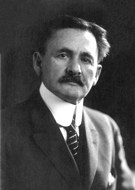
The importance of Huggins’ report on the Doppler effect from Sirius was more psychological than scientifically accurate, because it convinced the scientific community that the optical Doppler effect existed. Around this time the German astronomer Hermann Carl Vogel (1841 – 1907) of the Potsdam Observatory began working with a new spectrograph designed by Johann Zöllner from Leipzig [3] to improve the measurements of the radial velocity of stars (the speed along the line of sight). He was aware that the many values quoted by Huggins and others for stellar velocities were nearly the same as the uncertainties in their measurements. Vogel installed photographic capabilities in the telescope and spectrograph at the Potsdam Observatory [4] in 1887 and began making observations of Doppler line shifts in stars through 1890. He published an initial progress report in 1891, and then a definitive paper in 1892 that provided the first accurate stellar radial velocities [5]. Fifty years after Doppler read his paper to the Royal Bohemian Society of Science (in 1842 to a paltry crowd of only a few scientists), the Doppler effect had become an established workhorse of quantitative astrophysics. A laboratory demonstration of the optical Doppler effect was finally achieved in 1901 by Aristarkh Belopolsky (1854-1934), a Russian astronomer, by constructing a device with a narrow-linewidth light source and rapidly rotating mirrors [6].
White Dwarf
While measuring the position of Sirius to unprecedented precision, the German astronomer Friedrich Wilhelm Bessel (1784 – 1846) noticed a slow shift in its position. (This is the same Bessel as “Bessel function” fame, although the functions were originally developed by Daniel Bernoulli and Bessel later generalized them.) Bessel deduced that Sirius must have an unseen companion with an orbital of around 50 years. This companion was discovered by accident in 1862 during a test run of a new lens manufactured by the Clark&Sons glass manufacturing company prior to delivery to Northwestern University in Chicago. (The lens was originally ordered by the University of Mississippi in 1860, but after the Civil War broke out, the Massachusetts-based Clark company put it up for bid. Harvard wanted it, but Northwestern got it.) Sirius itself was redesignated Sirius A, while this new star was designated Sirius B (and sometimes called “The Pup”).
Fig. White dwarf and planet.
The Pup’s spectrum was measured in 1915 by Walter Adams (1876 – 1956) which put it in the newly-formed class of “white dwarf” stars that were very small but, unlike other types of dwarf stars, they had very hot (white) spectra. The deflection of the orbit of Sirius A allowed its mass to be estimated at about one solar mass, which was normal for a dwarf star. Furthermore, its brightness and surface temperature allowed its density to be estimated, but here an incredible number came out: the density of Sirius B was about 30,000 times greater than the density of the sun! Astronomers at the time thought that this was impossible, and Arthur Eddington, who was the expert in star formation, called it “nonsense”. This nonsense withstood all attempts to explain it for over a decade.
In 1926, R. H. Fowler (1889 – 1944) at Cambridge University in England applied the newly-developed theory of quantum mechanics and the Pauli exclusion principle to the problem of such ultra-dense matter. He found that the Fermi sea of electrons provided a type of pressure, called degeneracy pressure, that counteracted the gravitational pressure that threatened to collapse the star under its own weight. Several years later, Subrahmanyan Chandrasekhar calculated the upper limit for white dwarfs using relativistic effects and accurate density profiles and found that a white dwarf with a mass greater than about 1.5 times the mass of the sun would no longer be supported by the electron degeneracy pressure and would suffer gravitational collapse. At the time, the question of what it would collapse to was unknown, although it was later understood that it would collapse to a neutron star. Sirius B, at about one solar mass, is well within the stable range of white dwarfs.
But this was not the end of the story for Sirius B [7]. At around the time that Adams was measuring the spectrum of the white dwarf, Einstein was predicting that light emerging from a dense star would have its wavelengths gravitationally redshifted relative to its usual wavelength. This was one of the three classic tests he proposed for his new theory of General Relativity. (1 – The precession of the perihelion of Mercury. 2 – The deflection of light by gravity. 3 – The gravitational redshift of photons rising out of a gravity well.) Adams announced in 1925 (after the deflection of light by gravity had been confirmed by Eddington in 1919) that he had measured the gravitational redshift. Unfortunately, it was later surmised that he had not measured the gravitational effect but had actually measured Doppler-shifted spectra because of the rotational motion of the star. The true gravitational redshift of Sirius B was finally measured in 1971, although the redshift of another white dwarf, 40 Eridani B, had already been measured in 1954.
Static Interference
The quantum nature of light is an elusive quality that requires second-order experiments of intensity fluctuations to elucidate them, rather than using average values of intensity. But even in second-order experiments, the manifestations of quantum phenomenon are still subtle, as evidenced by an intense controversy that was launched by optical experiments performed in the 1950’s by a radio astronomer, Robert Hanbury Brown (1916 – 2002). (For the full story, see Chapter 4 in my book Interference from Oxford (2023) [8]).
Hanbury Brown (he never went by his first name) was born in Aruvankandu, India, the son of a British army officer. He never seemed destined for great things, receiving an unremarkable education that led to a degree in radio engineering from a technical college in 1935. He hoped to get a PhD in radio technology, and he even received a scholarship to study at Imperial College in London, when he was urged by the rector of the university, Sir Henry Tizard, to give up his plans and join an effort to develop defensive radar against a growing threat from Nazi Germany as it aggressively rearmed after abandoning the punitive Versailles Treaty. Hanbury Brown began the most exciting and unnerving five years of his life, right in the middle of the early development of radar defense, leading up to the crucial role it played in the Battle of Britain in 1940 and the Blitz from 1940 to 1941. Partly due to the success of radar, Hitler halted night-time raids in the Spring of 1941, and England escaped invasion.
In 1949, fourteen years after he had originally planned to start his PhD, Hanbury Brown enrolled at the relatively ripe age of 33 at the University of Manchester. Because of his background in radar, his faculty advisor told him to look into the new field of radio astronomy that was just getting started, and Manchester was a major player because it administrated the Jodrell Bank Observatory, which was one of the first and largest radio astronomy observatories in the World. Hanbury Brown was soon applying all he had learned about radar transmitters and receivers to the new field, focusing particularly on aspects of radio interferometry after Martin Ryle (1918 – 1984) at Cambridge with Derek Vonberg (1921 – 2015) developed the first radio interferometer to measure the angular size of the sun [9] and of radio sources on the Sun’s surface that were related to sunspots [10]. Despite the success of their measurements, their small interferometer was unable to measure the size of other astronomical sources. From Michelson’s formula for stellar interferometry, longer baselines between two separated receivers would be required to measure smaller angular sizes. For his PhD project, Hanbury Brown was given the task of designing a radio interferometer to resolve the two strongest radio sources in the sky, Cygnus A and Cassiopeia A, whose angular sizes were unknown. As he started the project, he was confronted with the problem of distributing a stable reference signal to receivers that might be very far apart, maybe even thousands of kilometers, a problem that had no easy solution.
After grappling with this technical problem for months without success, late one night in 1949 Hanbury Brown had an epiphany [11], wondering what would happen if the two separate radio antennas measured only intensities rather than fields. The intensity in a radio telescope fluctuates in time like random noise. If that random noise were measured at two separated receivers while trained on a common source, would those noise patterns look the same? After a few days considering this question, he convinced himself that the noise would indeed share common features, and the degree to which the two noise traces were similar should depend on the size of the source and the distance between the two receivers, just like Michelson’s fringe visibility. But his arguments were back-of-the-envelope, so he set out to find someone with the mathematical skills to do it more rigorously. He found Richard Twiss.
Richard Quentin Twiss (1920 – 2005), like Hanbury Brown, was born in India to British parents but had followed a more prestigious educational path, taking the Mathematical Tripos exam at Cambridge in 1941 and receiving his PhD from MIT in the United States in 1949. He had just returned to England, joining the research division of the armed services located north of London, when he received a call from Hanbury Brown at the Jodrell Bank radio astronomy laboratory in Manchester. Twiss travelled to meet Hanbury Brown in Manchester, who put him up in his flat in the neighboring town of Wilmslow. The two set up the mathematical assumptions behind the new “intensity interferometer” and worked late into the night. When Hanbury Brown finally went to bed, Twiss was still figuring the numbers. The next morning, the tall and lanky Twiss appeared in his silk dressing gown in the kitchen and told Hanbury Brown, “This idea of yours is no good, it doesn’t work”[12]—it would never be strong enough to detect the intensity from stars. However, after haggling over the details of some of the integrals, Hanbury Brown, and then finally Twiss, became convinced that the effect was real. Rather than fringe visibility, it was the correlation coefficient between two noise signals that would depend on the joint sizes of the source and receiver in a way that captured the same information as Michelson’s first-order fringe visibility. But because no coherent reference wave was needed for interferometric mixing, this new approach could be carried out across very large baseline distances.
After demonstrating the effect on astronomical radio sources, Hanbury Brown and Twiss took the next obvious step: optical stellar intensity interferometry. Their work had shown that photon noise correlations were analogous to Michelson fringe visibility, so the stellar intensity interferometer was expected to work similarly to the Michelson stellar interferometer—but with better stability over much longer baselines because it did not need a reference. An additional advantage was the simple light collecting requirements. Rather than needing a pair of massively expensive telescopes for high-resolution imaging, the intensity interferometer only needed to point two simple light collectors in a common direction. For this purpose, and to save money, Hanbury Brown selected two of the largest army-surplus anti-aircraft searchlights that he could find left over from the London Blitz. The lamps were removed and replaced with high-performance photomultipliers, and the units were installed on two train cars that could run along a railroad siding that crossed the Jodrell Bank grounds.
Fig. Stellar Interferometers: (Left) Michelson Stellar Field Interferometer. (Right) Hanbury Brown Twiss Stellar Intensity Interferometer.
The target of the first test of the intensity interferometer was Sirius, the Dog Star. Sirius was chosen because it is the brightest star in the night sky and was close to Earth at 8.6 light years and hence would be expected to have a relatively large angular size. The observations began at the start of winter in 1955, but the legendary English weather proved an obstacle. In addition to endless weeks of cloud cover, on many nights dew formed on the reflecting mirrors, making it necessary to install heaters. It took more than three months to make 60 operational attempts to accumulate a mere 18 hours of observations [13]. But it worked! The angular size of Sirius was measured for the first time. It subtended an angle of approximately 6 milliarcseconds (mas), which was well within the expected range for such a main sequence blue star. This angle is equivalent to observing a house on the Moon from the Earth. No single non-interferometric telescope on Earth, or in Earth orbit, has that kind of resolution, even today. Once again, Sirus was the testbed of a new observational technology. Hanbury Brown and Twiss went on the measure the diameters of dozens of stars.
Adaptive Optics
Any undergraduate optics student can tell you that bigger telescopes have higher spatial resolution. But this is only true up to a point. When telescope diameters become not much bigger than about 10 inches, the images they form start to dance, caused by thermal fluctuations in the atmosphere. Large telescopes can still get “lucky” at moments when the atmosphere is quiet, but this usually only happens for a fraction of a second before the fluctuation set in again. This is the primary reason that the Hubble Space Telescope was placed in Earth orbit above the atmosphere, and why the James Webb Space Telescope is flying a million miles away from the Earth. But that is not the end of Earth-based large telescoped. The Very Large Telescope (VLT) has a primary diameter of 8 meters, and the Extremely Large Telescope (ELT), coming online soon, has an even bigger diameter of 40 meters. How do these work under the atmospheric blanket? The answer is adaptive optics.
Adaptive optics uses active feedback to measure the dancing images caused by the atmosphere and uses the information to control a flexible array of mirror elements to exactly cancel out the effects of the atmospheric fluctuations. In the early days of adaptive-optics development, the applications were more military than astronomic, but advances made in imaging enemy satellites soon was released to the astronomers. The first civilian demonstrations of adaptive optics were performed in 1977 when researchers at Bell Labs [14] and at the Space Sciences Lab at UC Berkeley [15] each made astronomical demonstrations of improved seeing of the star Sirius using adaptive optics. The field developed rapidly after that, but once again Sirius had led the way.
Star Travel
The day is fast approaching when humans will begin thinking seriously of visiting nearby stars—not in person at first, but with unmanned spacecraft that can telemeter information back to Earth. Although Sirius is not the closest star to Earth—it is 8.6 lightyears away while Alpha Centauri is almost twice as close at only 4.2 lightyears away—it may be the best target for an unmanned spacecraft. The reason is its brightness.
Stardrive technology is still in its infancy—most of it is still on drawing boards. Therefore, the only “mature” technology we have today is light pressure on solar sails. Within the next 50 years or so we will have the technical ability to launch a solar sail towards a nearby star and accelerate it to a good fraction of the speed of light. The problem is decelerating the spaceship when it arrives at its destination, otherwise it will go zipping by with only a few seconds to make measurements after its long trek there.
Fig. NASA’s solar sail demonstrator unit (artist’s rendering).
A better idea is to let the star light push against the solar sail to decelerate it to orbital speed by the time it arrives. That way, the spaceship can orbit the target star for years. This is a possibility with Sirius. Because it is so bright, its light can decelerate the spaceship even when it is originally moving at relativistic speeds. By one calculation, the trip to Sirius, including the deceleration and orbital insertion, should only take about 69 years [16]. That’s just one lifetime. Signals could be beaming back from Sirius by as early as 2100—within the lifetimes of today’s children.
[2] W. Huggins, “Further observations on the spectra of some of the stars and nebulae, with an attempt to determine therefrom whether these bodies are moving towards or from the earth, also observations on the spectra of the sun and of comet II,” Philos. Trans. R. Soc. London vol. 158, pp. 529-564, 1868. The correct value is -5.5 km/sec approaching Earth. Huggins got the magnitude and even the sign wrong.
[3] in Hearnshaw, The Analysis of Starlight (Cambridge University Press, 2014), pg. 89
[4] The Potsdam Observatory was where the American Albert Michelson built his first interferometer while studying with Helmholtz in Berlin.
[5] Vogel, H. C. Publik. der astrophysik. Observ. Potsdam1: 1. (1892)
[6] A. Belopolsky, “On an apparatus for the laboratory demonstration of the Doppler-Fizeau principle,” Astrophysical Journal, vol. 13, pp. 15-24, Jan 1901.
[9] M. Ryle and D. D. Vonberg, “Solar Radiation on 175 Mc/sec,” Nature, vol. 158 (1946): pp. 339-340.; K. I. Kellermann and J. M. Moran, “The development of high-resolution imaging in radio astronomy,” Annual Review of Astronomy and Astrophysics, vol. 39, (2001): pp. 457-509.
[10] M. Ryle, ” Solar radio emissions and sunspots,” Nature, vol. 161, no. 4082 (1948): pp. 136-136.
[11] R. H. Brown, The intensity interferometer; its application to astronomy (London, New York, Taylor & Francis; Halsted Press, 1974).
[12] R. H. Brown, Boffin : A personal story of the early days of radar and radio astronomy (Adam Hilger, 1991), p. 106.
[13] R. H. Brown and R. Q. Twiss. ” Test of a new type of stellar interferometer on Sirius.” Nature178, no. 4541 (1956): pp. 1046-1048.
[14] S. L. McCall, T. R. Brown, and A. Passner, “IMPROVED OPTICAL STELLAR IMAGE USING A REAL-TIME PHASE-CORRECTION SYSTEM – INITIAL RESULTS,” Astrophysical Journal, vol. 211, no. 2, pp. 463-468, (1977)
[15] A. Buffington, F. S. Crawford, R. A. Muller, and C. D. Orth, “1ST OBSERVATORY RESULTS WITH AN IMAGE-SHARPENING TELESCOPE,” Journal of the Optical Society of America, vol. 67, no. 3, pp. 304-305, 1977 (1977)
The synopses of the first chapters can be found in my previous blog. Here are previews of the final chapters.
Chapter 6. Across the Universe: Exoplanets, Black Holes and Gravitational Waves
Stellar interferometry is opening new vistas of astronomy, exploring the wildest occupants of our universe, from colliding black holes half-way across the universe (LIGO) to images of neighboring black holes (EHT) to exoplanets near Earth that may harbor life.
Image of the supermassive black hole in M87 from Event Horizon Telescope.
Across the Universe: Gravitational Waves, Black Holes and the Search for Exoplanets describes the latest discoveries of interferometry in astronomy including the use of nulling interferometry in the Very Large Telescope Interferometer (VLTI) to detect exoplanets orbiting distant stars. The much larger Event Horizon Telescope (EHT) used long baseline interferometry and closure phase advanced by Roger Jenison to make the first image of a black hole. The Laser Interferometric Gravitational Observatory (LIGO) represented a several-decade-long drive to detect the first gravitational waves first predicted by Albert Einstein a hundred years ago.
Chapter 7. Two Faces of Microscopy: Diffraction and Interference
From the astronomically large dimensions of outer space to the microscopically small dimensions of inner space, optical interference pushes the resolution limits of imaging.
Two Faces of Microscopy: Diffraction and Interference describes the development of microscopic principles starting with Joseph Fraunhofer and the principle of diffraction gratings that was later perfected by Henry Rowland for high-resolution spectroscopy. The company of Carl Zeiss advanced microscope technology after enlisting the help of Ernst Abbe who formed a new theory of image formation based on light interference. These ideas were extended by Fritz Zernike in the development of phase-contrast microscopy. The ultimate resolution of microscopes, defined by Abbe and known as the Abbe resolution limit, turned out not to be a fundamental limit, but was surpassed by super-resolution microscopy using concepts of interference microscopy and structured illumination.
Chapter 8. Holographic Dreams of Princess Leia: Crossing Beams
The coherence of laser light is like a brilliant jewel that sparkles in the darkness, illuminating life, probing science and projecting holograms in virtual worlds.
Ted Maiman
Holographic Dreams of Princess Leia: Crossing Beams presents the history of holography, beginning with the original ideas of Denis Gabor who invented optical holography as a means to improve the resolution of electron microscopes. Holography became mainstream after the demonstrations by Emmett Leith and Juris Upatnieks using lasers that were first demonstrated by Ted Maiman at Hughes Research Lab after suggestions by Charles Townes on the operating principles of the optical maser. Dynamic holography takes place in crystals that exhibit the photorefractive effect that are useful for adaptive interferometry. Holographic display technology is under development, using ideas of holography merged with light-field displays that were first developed by Gabriel Lippmann.
Chapter 9. Photon Interference: The Foundations of Quantum Communication and Computing
What is the image of one photon interfering? Better yet, what is the image of two photons interfering? The answer to this crucial question laid the foundation for quantum communication.
Photon Interference: The Foundations of Quantum Communication moves the story of interferometry into the quantum realm, beginning with the Einstein-Podolski-Rosen paradox and the principle of quantum entanglement that was refined by David Bohm who tried to banish uncertainty from quantum theory. John Bell and John Clauser pushed the limits of what can be known from quantum measurement as Clauser tested Bell’s inequalities, confirming the fundamental nonlocal character of quantum systems. Leonard Mandel pushed quantum interference into the single-photon regime, discovering two-photon interference fringes that illustrated deep concepts of quantum coherence. Quantum communication began with quantum cryptography and developed into quantum teleportation that can provide the data bus of future quantum computers.
Chapter 10. The Quantum Advantage: Interferometric Computing
There is almost no technical advantage better than having exponential resources at hand. The exponential resources of quantum interference provide that advantage to quantum computing which is poised to usher in a new era of quantum information science and technology.
David Deutsch.
The Quantum Advantage: Interferometric Computing describes the development of quantum algorithms and quantum computing beginning with the first quantum algorithm invented by David Deutsch as a side effect of his attempt to prove the multiple world interpretation of quantum theory. Peter Shor found a quantum algorithm that could factor the product of primes and that threatened all secure communications in the world. Once the usefulness of quantum algorithms was recognized, quantum computing hardware ideas developed rapidly into quantum circuits supported by quantum logic gates. The limitation of optical interactions, that hampered the development of controlled quantum gates, led to the proposal of linear optical quantum computing and boson sampling in a complex cascade of single-photon interferometers that has been used to demonstrate quantum supremacy, also known as quantum computational advantage, using photonic integrated circuits.
From Oxford Press: Interference
Stories about the trials and toils of the scientists and engineers who tamed light and used it to probe the universe.
This history of interferometry has many surprising back stories surrounding the scientists who discovered and explored one of the most important aspects of the physics of light—interference. From Thomas Young who first proposed the law of interference, and Augustin Fresnel and Francois Arago who explored its properties, to Albert Michelson, who went almost mad grappling with literal firestorms surrounding his work, these scientists overcame personal and professional obstacles on their quest to uncover light’s secrets. The book’s stories, told around the topic of optics, tells us something more general about human endeavor as scientists pursue science.
Interference: The History of Optical Interferometry and the Scientists who Tamed Light, was published Ag. 6 and is available at Oxford University Press and Amazon. Here is a brief preview of the frist several chapters:
Chapter 1. Thomas Young Polymath: The Law of Interference
Thomas Young was the ultimate dabbler, his interests and explorations ranged far and wide, from ancient egyptology to naval engineering, from physiology of perception to the physics of sound and light. Yet unlike most dabblers who accomplish little, he made original and seminal contributions to all these fields. Some have called him the “Last Man Who Knew Everything”.
Thomas Young. The Law of Interference.
The chapter, Thomas Young Polymath: The Law of Interference, begins with the story of the invasion of Egypt in 1798 by Napoleon Bonaparte as the unlikely link among a set of epic discoveries that launched the modern science of light. The story of interferometry passes from the Egyptian campaign and the discovery of the Rosetta Stone to Thomas Young. Young was a polymath, known for his facility with languages that helped him decipher Egyptian hieroglyphics aided by the Rosetta Stone. He was also a city doctor who advised the admiralty on the construction of ships, and he became England’s premier physicist at the beginning of the nineteenth century, building on the wave theory of Huygens, as he challenged Newton’s particles of light. But his theory of the wave nature of light was controversial, attracting sharp criticism that would pass on the task of refuting Newton to a new generation of French optical physicists.
Chapter 2. The Fresnel Connection: Particles versus Waves
Augustin Fresnel was an intuitive genius whose talents were almost squandered on his job building roads and bridges in the backwaters of France until he was discovered and rescued by Francois Arago.
The Fresnel Connection: Particles versus Waves describes the campaign of Arago and Fresnel to prove the wave nature of light based on Fresnel’s theory of interfering waves in diffraction. Although the discovery of the polarization of light by Etienne Malus posed a stark challenge to the undulationists, the application of wave interference, with the superposition principle of Daniel Bernoulli, provided the theoretical framework for the ultimate success of the wave theory. The final proof came through the dramatic demonstration of the Spot of Arago.
Chapter 3. At Light Speed: The Birth of Interferometry
There is no question that Francois Arago was a swashbuckler. His life’s story reads like an adventure novel as he went from being marooned in hostile lands early in his career to becoming prime minister of France after the 1848 revolutions swept across Europe.
At Light Speed: The Birth of Interferometry tells how Arago attempted to use Snell’s Law to measure the effect of the Earth’s motion through space but found no effect, in contradiction to predictions using Newton’s particle theory of light. Direct measurements of the speed of light were made by Hippolyte Fizeau and Leon Foucault who originally began as collaborators but had an epic falling-out that turned into an intense competition. Fizeau won priority for the first measurement, but Foucault surpassed him by using the Arago interferometer to measure the speed of light in air and water with increasing accuracy. Jules Jamin later invented one of the first interferometric instruments for use as a refractometer.
Chapter 4. After the Gold Rush: The Trials of Albert Michelson
No name is more closely connected to interferometry than that of Albert Michelson. He succeeded, sometimes at great personal cost, in launching interferometric metrology as one of the most important tools used by scientists today.
Albert A. Michelson, 1907 Nobel Prize. Image Credit.
After the Gold Rush: The Trials of Albert Michelson tells the story of Michelson’s youth growing up in the gold fields of California before he was granted an extraordinary appointment to Annapolis by President Grant. Michelson invented his interferometer while visiting Hermann von Helmholtz in Berlin, Germany, as he sought to detect the motion of the Earth through the luminiferous ether, but no motion was detected. After returning to the States and a faculty position at Case University, he met Edward Morley, and the two continued the search for the Earth’s motion, concluding definitively its absence. The Michelson interferometer launched a menagerie of interferometers (including the Fabry-Perot interferometer) that ushered in the golden age of interferometry.
Chapter 5. Stellar Interference: Measuring the Stars
Learning from his attempts to measure the speed of light through the ether, Michelson realized that the partial coherence of light from astronomical sources could be used to measure their sizes. His first measurements using the Michelson Stellar Interferometer launched a major subfield of astronomy that is one of the most active today.
R Hanbury Brown
Stellar Interference: Measuring the Stars brings the story of interferometry to the stars as Michelson proposed stellar interferometry, first demonstrated on the Galilean moons of Jupiter, followed by an application developed by Karl Schwarzschild for binary stars, and completed by Michelson with observations encouraged by George Hale on the star Betelgeuse. However, the Michelson stellar interferometry had stability limitations that were overcome by Hanbury Brown and Richard Twiss who developed intensity interferometry based on the effect of photon bunching. The ultimate resolution of telescopes was achieved after the development of adaptive optics that used interferometry to compensate for atmospheric turbulence.
And More
The last 5 chapters bring the story from Michelson’s first stellar interferometer into the present as interferometry is used today to search for exoplanets, to image distant black holes half-way across the universe and to detect gravitational waves using the most sensitive scientific measurement apparatus ever devised.
Chapter 6. Across the Universe: Exoplanets, Black Holes and Gravitational Waves
Moving beyond the measurement of star sizes, interferometry lies at the heart of some of the most dramatic recent advances in astronomy, including the detection of gravitational waves by LIGO, the imaging of distant black holes and the detection of nearby exoplanets that may one day be visited by unmanned probes sent from Earth.
Chapter 7. Two Faces of Microscopy: Diffraction and Interference
The complement of the telescope is the microscope. Interference microscopy allows invisible things to become visible and for fundamental limits on image resolution to be blown past with super-resolution at the nanoscale, revealing the intricate workings of biological systems with unprecedented detail.
Chapter 8. Holographic Dreams of Princess Leia: Crossing Beams
Holography is the direct legacy of Young’s double slit experiment, as coherent sources of light interfere to record, and then reconstruct, the direct scattered fields from illuminated objects. Holographic display technology promises to revolutionize virtual reality.
Chapter 9. Photon Interference: The Foundations of Quantum Communication and Computing
Quantum information science, at the forefront of physics and technology today, owes much of its power to the principle of interference among single photons.
Chapter 10. The Quantum Advantage: Interferometric Computing
Photonic quantum systems have the potential to usher in a new information age using interference in photonic integrated circuits.
A popular account of the trials and toils of the scientists and engineers who tamed light and used it to probe the universe.
When Galileo trained his crude telescope on the planet Jupiter, hanging above the horizon in 1610, and observed moons orbiting a planet other than Earth, it created a quake whose waves have rippled down through the centuries to today. Never had such hard evidence been found that supported the Copernican idea of non-Earth-centric orbits, freeing astronomy and cosmology from a thousand years of error that shaded how people thought.
The Earth, after all, was not the center of the Universe.
Galileo’s moons: the Galilean Moons—Io, Europa, Ganymede, and Callisto—have drawn our eyes skyward now for over 400 years. They have been the crucible for numerous scientific discoveries, serving as a test bed for new ideas and new techniques, from the problem of longitude to the speed of light, from the birth of astronomical interferometry to the beginnings of exobiology. Here is a short history of Galileo’s Moons in the history of physics.
Galileo (1610): Celestial Orbits
In late 1609, Galileo (1564 – 1642) received an unwelcome guest to his home in Padua—his mother. She was not happy with his mistress, and she was not happy with his chosen profession, but she was happy to tell him so. By the time she left in early January 1610, he was yearning for something to take his mind off his aggravations, and he happened to point his new 20x telescope in the direction of the planet Jupiter hanging above the horizon [1]. Jupiter appeared as a bright circular spot, but nearby were three little stars all in line with the planet. The alignment caught his attention, and when he looked again the next night, the position of the stars had shifted. On successive nights he saw them shift again, sometimes disappearing into Jupiter’s bright disk. Several days later he realized that there was a fourth little star that was also behaving the same way. At first confused, he had a flash of insight—the little stars were orbiting the planet. He quickly understood that just as the Moon orbited the Earth, these new “Medicean Planets” were orbiting Jupiter. In March 1610, Galileo published his findings in Siderius Nuncius (The Starry Messenger).
Page from Galileo’s Starry Messenger showing the positions of the moon of Jupiter
It is rare in the history of science for there not to be a dispute over priority of discovery. Therefore, by an odd chance of fate, on the same nights that Galileo was observing the moons of Jupiter with his telescope from Padua, the German astronomer Simon Marius (1573 – 1625) also was observing them through a telescope of his own from Bavaria. It took Marius four years to publish his observations, long after Galileo’s Siderius had become a “best seller”, but Marius took the opportunity to claim priority. When Galileo first learned of this, he called Marius “a poisonous reptile” and “an enemy of all mankind.” But harsh words don’t settle disputes, and the conflicting claims of both astronomers stood until the early 1900’s when a scientific enquiry looked at the hard evidence. By that same odd chance of fate that had compelled both men to look in the same direction around the same time, the first notes by Marius in his notebooks were dated to a single day after the first notes by Galileo! Galileo’s priority survived, but Marius may have had the last laugh. The eternal names of the “Galilean” moons—Io, Europe, Ganymede and Callisto—were given to them by Marius.
Picard and Cassini (1671): Longitude
The 1600’s were the Age of Commerce for the European nations who relied almost exclusively on ships and navigation. While latitude (North-South) was easily determined by measuring the highest angle of the sun above the southern horizon, longitude (East-West) relied on clocks which were notoriously inaccurate, especially at sea.
The Problem of Determining Longitude at Sea is the subject of Dava Sobel’s thrilling book Longitude (Walker, 1995) [2] where she reintroduced the world to what was once the greatest scientific problem of the day. Because almost all commerce was by ships, the determination of longitude at sea was sometimes the difference between arriving safely in port with a cargo or being shipwrecked. Galileo knew this, and later in his life he made a proposal to the King of Spain to fund a scheme to use the timings of the eclipses of his moons around Jupiter to serve as a “celestial clock” for ships at sea. Galileo’s grant proposal went unfunded, but the possibility of using the timings of Jupiter’s moons for geodesy remained an open possibility, one which the King of France took advantage of fifty years later.
In 1671 the newly founded Academie des Sciences in Paris funded an expedition to the site of Tycho Brahe’s Uranibourg Observatory in Hven, Denmark, to measure the time of the eclipses of the Galilean moons observed there to be compared the time of the eclipses observed in Paris by Giovanni Cassini (1625 – 1712). When the leader of the expedition, Jean Picard (1620 – 1682), arrived in Denmark, he engaged the services of a local astronomer, Ole Rømer (1644 – 1710) to help with the observations of over 100 eclipses of the Galilean moon Io by the planet Jupiter. After the expedition returned to France, Cassini and Rømer calculated the time differences between the observations in Paris and Hven and concluded that Galileo had been correct. Unfortunately, observing eclipses of the tiny moon from the deck of a ship turned out not to be practical, so this was not the long-sought solution to the problem of longitude, but it contributed to the early science of astrometry (the metrical cousin of astronomy). It also had an unexpected side effect that forever changed the science of light.
Ole Rømer (1676): The Speed of Light
Although the differences calculated by Cassini and Rømer between the times of the eclipses of the moon Io between Paris and Hven were small, on top of these differences was superposed a surprisingly large effect that was shared by both observations. This was a systematic shift in the time of eclipse that grew to a maximum value of 22 minutes half a year after the closest approach of the Earth to Jupiter and then decreased back to the original time after a full year had passed and the Earth and Jupiter were again at their closest approach. At first Cassini thought the effect might be caused by a finite speed to light, but he backed away from this conclusion because Galileo had shown that the speed of light was unmeasurably fast, and Cassini did not want to gainsay the old master.
Ole Rømer
Rømer, on the other hand, was less in awe of Galileo’s shadow, and he persisted in his calculations and concluded that the 22 minute shift was caused by the longer distance light had to travel when the Earth was farthest away from Jupiter relative to when it was closest. He presented his results before the Academie in December 1676 where he announced that the speed of light, though very large, was in fact finite. Unfortnately, Rømer did not have the dimensions of the solar system at his disposal to calculate an actual value for the speed of light, but the Dutch mathematician Huygens did.
When Christian Huygens read the proceedings of the Academie in which Rømer had presented his findings, he took what he knew of the radius of Earth’s orbit and the distance to Jupiter and made the first calculation of the speed of light. He found a value of 220,000 km/second (kilometers did not exist yet, but this is the equivalent of what he calculated). This value is 26 percent smaller than the true value, but it was the first time a number was given to the finite speed of light—based fundamentally on the Galilean moons. For a popular account of the story of Picard and Rømer and Huygens and the speed of light, see Ref. [3].
Michelson (1891): Astronomical Interferometry
Albert Michelson (1852 – 1931) was the first American to win the Nobel Prize in Physics. He received the award in 1907 for his work to replace the standard meter, based on a bar of metal housed in Paris, with the much more fundamental wavelength of red light emitted by Cadmium atoms. His work in Paris came on the heels of a new and surprising demonstration of the use of interferometry to measure the size of astronomical objects.
Albert Michelson
The wavelength of light (a millionth of a meter) seems ill-matched to measuring the size of astronomical objects (thousands of meters) that are so far from Earth (billions of meters). But this is where optical interferometry becomes so important. Michelson realized that light from a distant object, like a Galilean moon of Jupiter, would retain some partial coherence that could be measured using optical interferometry. Furthermore, by measuring how the interference depended on the separation of slits placed on the front of a telescope, it would be possible to determine the size of the astronomical object.
From left to right: Walter Adams, Albert Michelson, Walther Mayer, Albert Einstein, Max Ferrand, and Robert Milliken. Photo taken at Caltech.
In 1891, Michelson traveled to California where the Lick Observatory was poised high above the fog and dust of agricultural San Jose (a hundred years before San Jose became the capitol of high-tech Silicon Valley). Working with the observatory staff, he was able to make several key observations of the Galilean moons of Jupiter. These were just close enough that their sizes could be estimated (just barely) from conventional telescopes. Michelson found from his calculations of the interference effects that the sizes of the moons matched the conventional sizes to within reasonable error. This was the first demonstration of astronomical interferometry which has burgeoned into a huge sub-discipline of astronomy today—based originally on the Galilean moons [4].
Pioneer (1973 – 1974): The First Tour
Pioneer 10 was launched on March 3, 1972 and made its closest approach to Jupiter on Dec. 3, 1973. Pioneer 11 was launched on April 5, 1973 and made its closest approach to Jupiter on Dec. 3, 1974 and later was the first spacecraft to fly by Saturn. The Pioneer spacecrafts were the first to leave the solar system (there have now been 5 that have left, or will leave, the solar system). The cameras on the Pioneers were single-pixel instruments that made line-scans as the spacecraft rotated. The point light detector was a Bendix Channeltron photomultiplier detector, which was a vacuum tube device (yes vacuum tube!) operating at a single-photon detection efficiency of around 10%. At the time of the system design, this was a state-of-the-art photon detector. The line scanning was sufficient to produce dramatic photographs (after extensive processing) of the giant planets. The much smaller moons were seen with low resolution, but were still the first close-ups ever to be made of Galileo’s moons.
Voyager (1979): The Grand Tour
Voyager 1 was launched on Sept. 5, 1977 and Voyager 2 was launched on August 20, 1977. Although Voyager 1 was launched second, it was the first to reach Jupiter with closest approach on March 5, 1979. Voyager 2 made its closest approach to Jupiter on July 9, 1979.
In the Fall of 1979, I had the good fortune to be an undergraduate at Cornell University when Carl Sagan gave an evening public lecture on the Voyager fly-bys, revealing for the first time the amazing photographs of not only Jupiter but of the Galilean Moons. Sitting in the audience listening to Sagan, a grand master of scientific story telling, made you feel like you were a part of history. I have never been so convinced of the beauty and power of science and technology as I was sitting in the audience that evening.
The camera technology on the Voyagers was a giant leap forward compared to the Pioneer spacecraft. The Voyagers used cathode ray vidicon cameras, like those used in television cameras of the day, with high-resolution imaging capabilities. The images were spectacular, displaying alien worlds in high-def for the first time in human history: volcanos and lava flows on the moon of Io; planet-long cracks in the ice-covered surface of Europa; Callisto’s pock-marked surface; Ganymede’s eerie colors.
The Voyager’s discoveries concerning the Galilean Moons were literally out of this world. Io was discovered to be a molten planet, its interior liquified by tidal-force heating from its nearness to Jupiter, spewing out sulfur lava onto a yellowed terrain pockmarked by hundreds of volcanoes, sporting mountains higher than Mt. Everest. Europa, by contrast, was discovered to have a vast flat surface of frozen ice, containing no craters nor mountains, yet fractured by planet-scale ruptures stained tan (for unknown reasons) against the white ice. Ganymede, the largest moon in the solar system, is a small planet, larger than Mercury. The Voyagers revealed that it had a blotchy surface with dark cratered patches interspersed with light smoother patches. Callisto, again by contrast, was found to be the most heavily cratered moon in the solar system, with its surface pocked by countless craters.
Galileo (1995): First in Orbit
The first mission to orbit Jupiter was the Galileo spacecraft that was launched, not from the Earth, but from Earth orbit after being delivered there by the Space Shuttle Atlantis on Oct. 18, 1989. Galileo arrived at Jupiter on Dec. 7, 1995 and was inserted into a highly elliptical orbit that became successively less eccentric on each pass. It orbited Jupiter for 8 years before it was purposely crashed into the planet (to prevent it from accidentally contaminating Europa that may support some form of life).
Galileo made many close passes to the Galilean Moons, providing exquisite images of the moon surfaces while its other instruments made scientific measurements of mass and composition. This was the first true extended study of Galileo’s Moons, establishing the likely internal structures, including the liquid water ocean lying below the frozen surface of Europa. As the largest body of liquid water outside the Earth, it has been suggested that some form of life could have evolved there (or possibly been seeded by meteor ejecta from Earth).
Juno (2016): Still Flying
The Juno spacecraft was launched from Cape Canaveral on Aug. 5, 2011 and entered a Jupiter polar orbit on July 5, 2016. The mission has been producing high-resolution studies of the planet. The mission was extended in 2021 to last to 2025 to include several close fly-bys of the Galilean Moons, especially Europa, which will be the object of several upcoming missions because of the possibility for the planet to support evolved life. These future missions include NASA’s Europa Clipper Mission, the ESA’s Jupiter Icy Moons Explorer, and the Io Volcano Observer.
Epilog (2060): Colonization of Callisto
In 2003, NASA identified the moon Callisto as the proposed site of a manned base for the exploration of the outer solar system. It would be the next most distant human base to be established after Mars, with a possible start date by the mid-point of this century. Callisto was chosen because it is has a low radiation level (being the farthest from Jupiter of the large moons) and is geologically stable. It also has a composition that could be mined to manufacture rocket fuel. The base would be a short-term way-station (crews would stay for no longer than a month) for refueling before launching and using a gravity assist from Jupiter to sling-shot spaceships to the outer planets.
By David D. Nolte, May 29, 2023
[1] See Chapter 2, A New Scientist: Introducing Galileo, in David D. Nolte, Galileo Unbound (Oxford University Press, 2018).
[2] Dava Sobel, Longitude: The True Story of a Lone Genius who Solved the Greatest Scientific Problem of his Time (Walker, 1995)
[3] See Chap. 1, Thomas Young Polymath: The Law of Interference, in David D. Nolte, Interference: The History of Optical Interferometry and the Scientists who Tamed Light (Oxford University Press, 2023)
[4] See Chapter 5, Stellar Interference: Measuring the Stars, in David D. Nolte, Interference: The History of Optical Interferometry and the Scientists who Tamed Light (Oxford University Press, 2023).
Read more in Books by David Nolte at Oxford University Press