March 23, 2022June 1, 2023 by David D. Nolte

The Physics of Starflight: Proxima Centauri b or Bust!

The ability to travel to the stars has been one of mankind’s deepest desires. Ever since we learned that we are just one world in a vast universe of limitless worlds, we have yearned to visit some of those others. Yet nature has thrown up an almost insurmountable barrier to that desire–the speed of light. Only by traveling at or near the speed of light may we venture to far-off worlds, and even then, decades or centuries will pass during the voyage. The vast distances of space keep all the worlds isolated–possibly for the better.

Yet the closest worlds are not so far away that they will always remain out of reach. The very limit of the speed of light provides ways of getting there within human lifetimes. The non-intuitive effects of special relativity come to our rescue, and we may yet travel to the closest exoplanet we know of.

Proxima Centauri b

The closest habitable Earth-like exoplanet is Proxima Centauri b, orbiting the red dwarf star Proxima Centauri that is about 4.2 lightyears away from Earth. The planet has a short orbital period of only about 11 Earth days, but the dimness of the red dwarf puts the planet in what may be a habitable zone where water is in liquid form. Its official discovery date was August 24, 2016 by the European Southern Observatory in the Atacama Desert of Chile using the Doppler method. The Alpha Centauri system is a three-star system, and even before the discovery of the planet, this nearest star system to Earth was the inspiration for the Hugo-Award winning sci-fi trilogy The Three Body Problem by Chinese author Liu Cixin, originally published in 2008.

It may seem like a coincidence that the closest Earth-like planet to Earth is in the closest star system to Earth, but it says something about how common such exoplanets may be in our galaxy.

Artist’s rendition of Proxima Centauri b. From WikiCommons.

Breakthrough Starshot

There are already plans to send centimeter-sized spacecraft to Alpha Centauri. One such project that has received a lot of press is Breakthrough Starshot, a project of the Breakthrough Initiatives. Breakthrough Starshot would send around 1000 centimeter-sized camera-carrying laser-fitted spacecraft with 5-meter-diameter solar sails propelled by a large array of high-power lasers. The reason there are so many of these tine spacecraft is because of the collisions that are expected to take place with interstellar dust during the voyage. It is possible that only a few dozen of the craft will finally make it to Alpha Centauri intact.

Relative locations of the stars of the Alpha Centauri system. From ScienceNews.

As these spacecraft fly by the Alpha Centauri system, possibly within one hundred million miles of Proxima Centauri b, their tiny HR digital cameras will take pictures of the planet’s surface with enough resolution to see surface features. The on-board lasers will then transmit the pictures back to Earth. The travel time to the planet is expected to be 20 or 30 years, plus the four years for the laser information to make it back to Earth. Therefore, it would take a quarter century after launch to find out if Proxima Centauri b is habitable or not. The biggest question is whether it has an atmosphere. The red dwarf it orbits sends out catastrophic electromagnetic bursts that could strip the planet of its atmosphere thus preventing any chance for life to evolve or even to be sustained there if introduced.

There are multiple projects under consideration for travel to the Alpha Centauri systems. Even NASA has a tentative mission plan called the 2069 Mission (100 year anniversary of the Moon landing). This would entail a single spacecraft with a much larger solar sail than the small starshot units. Some of the mission plans proposed star-drive technology, such as nuclear propulsion systems, rather than light sails. Some of these designs could sustain a 1-g acceleration throughout the entire mission. It is intriguing to do the math on what such a mission could look like, in terms of travel time. Could we get an unmanned probe to Alpha Centauri in a matter of years? Let’s find out.

Special Relativity of Acceleration

The most surprising aspect of deriving the properties of relativistic acceleration using special relativity is that it works at all. We were all taught as young physicists that special relativity deals with inertial frames in constant motion. So the idea of frames that are accelerating might first seem to be outside the scope of special relativity. But one of Einstein’s key insights, as he sought to extend special relativity towards a more general theory, was that one can define a series of instantaneously inertial co-moving frames relative to an accelerating body. In other words, at any instant in time, the accelerating frame has an inertial co-moving frame. Once this is defined, one can construct invariants, just as in usual special relativity. And these invariants unlock the full mathematical structure of accelerating objects within the scope of special relativity.

For instance, the four-velocity and the four-acceleration in a co-moving frame for an object accelerating at g are given by

The object is momentarily stationary in the co-moving frame, which is why the four-velocity has only the zeroth component, and the four-acceleration has simply g for its first component.

Armed with these four-vectors, one constructs the invariants

and

This last equation is solved for the specific co-moving frame as

But the invariant is more general, allowing the expression

which yields

From these, putting them all together, one obtains the general differential equations for the change in velocity as a set of coupled equations

The solution to these equations is

where the unprimed frame is the lab frame (or Earth frame), and the primed frame is the frame of the accelerating object, for instance a starship heading towards Alpha Centauri. These equations allow one to calculate distances, times and speeds as seen in the Earth frame as well as the distances, times and speeds as seen in the starship frame. If the starship is accelerating at some acceleration g’ other than g, then the results are obtained simply by replacing g by g’ in the equations.

Relativistic Flight

It turns out that the acceleration due to gravity on our home planet provides a very convenient (but purely coincidental) correspondence

With a similarly convenient expression

These considerably simplify the math for a starship accelerating at g.

Let’s now consider a starship accelerating by g for the first half of the flight to Alpha Centauri, turning around and decelerating at g for the second half of the flight, so that the starship comes to a stop at its destination. The equations for the times to the half-way point are

This means at the midpoint that 1.83 years have elapsed on the starship, and about 3 years have elapsed on Earth. The total time to get to Alpha Centauri (and come to a stop) is then simply

It is interesting to look at the speed at the midpoint. This is obtained by

which is solved to give

This amazing result shows that the starship is traveling at 95% of the speed of light at the midpoint when accelerating at the modest value of g for about 3 years. Of course, the engineering challenges for providing such an acceleration for such a long time are currently prohibitive … but who knows? There is a lot of time ahead of us for technology to advance to such a point in the next century or so.

Figure. Time lapsed inside the spacecraft and on Earth for the probe to reach Alpha Centauri as a function of the acceleration of the craft. At 10 g’s, the time elapsed on Earth is a little less than 5 years. However, the signal sent back will take an additional 4.37 years to arrive for a total time of about 9 years.

Matlab alphacentaur.m

% alphacentaur.m
clear
format compact

g0 = 1;
L = 4.37;

for loop = 1:100
    
    g = 0.1*loop*g0;
    
    taup = (1/g)*acosh(g*L/2 + 1);
    tearth = (1/g)*sinh(g*taup);
    
    tauspacecraft(loop) = 2*taup;
    tlab(loop) = 2*tearth;
    
    acc(loop) = g;
    
end

figure(1)
loglog(acc,tauspacecraft,acc,tlab,'LineWidth',2)
legend('Space Craft','Earth Frame','FontSize',18)
xlabel('Acceleration (g)','FontSize',18)
ylabel('Time (years)','FontSize',18)
dum = set(gcf,'Color','White');
H = gca;
H.LineWidth = 2;
H.FontSize = 18;

To Centauri and Beyond

Once we get unmanned probes to Alpha Centauri, it opens the door to star systems beyond. The next closest are Barnards star at 6 Ly away, Luhman 16 at 6.5 Ly, Wise at 7.4 Ly, and Wolf 359 at 7.9 Ly. Several of these are known to have orbiting exoplanets. Ross 128 at 11 Ly and Lyuten at 12.2 Ly have known earth-like planets. There are about 40 known earth-like planets within 40 lightyears from Earth, and likely there are more we haven’t found yet. It is almost inconceivable that none of these would have some kind of life. Finding life beyond our solar system would be a monumental milestone in the history of science. Perhaps that day will come within this century.

By David D. Nolte, March 23, 2022

Surfing on a Black Hole: Accretion Disk Death Spiral

The most energetic physical processes in the universe (shy of the Big Bang itself) are astrophysical jets. These are relativistic beams of ions and radiation that shoot out across intergalactic space, emitting nearly the full spectrum of electromagnetic radiation, seen as quasars (quasi-stellar objects) that are thought to originate from supermassive black holes at the center of distant galaxies. The most powerful jets emit more energy than the light from a thousand Milky Way galaxies.

Where can such astronomical amounts of energy come from?

Black Hole Accretion Disks

The potential wells of black holes are so deep and steep, that they attract matter from their entire neighborhood. If a star comes too close, the black hole can rip the hydrogen and helium atoms off the star’s surface and suck them into a death spiral that can only end in oblivion beyond the Schwarzschild radius.

However, just before they disappear, these atoms and ions make one last desperate stand to resist the inevitable pull, and they park themselves near an orbit that is just stable enough that they can survive many orbits before they lose too much energy, through collisions with the other atoms and ions, and resume their in-spiral. This last orbit, called the inner-most stable circular orbit (ISCO), is where matter accumulates into an accretion disk.

Fig. 1 Artist’s rendering of a black hole pulling matter from a near-by star where it accumulates in the accretion disk just outside the black hole Schwarzschild radius. (Credit: Wikipedia)

Fig. 2 The famous first image of the black hole in M87 galaxy made by the Event Horizon Telescope collaboration. The bright ring surrounding the “shadow” is the light emitted from the accretion disk.

Fig. 3 Explanation of the image of the accretion disk around a black hole. (You have to watch the simulations at NASA.)

The Innermost Stable Circular Orbit (ISCO)

At what radius is the inner-most stable circular orbit? To find out, write the energy equation of a particle orbiting a black hole with an effective potential function as

where the effective potential is

The first two terms of the effective potential are the usual Newtonian terms that include the gravitational potential and the repulsive contribution from the angular momentum that normally prevents the mass from approaching the origin. The third term is the GR term that is attractive and overcomes the centrifugal barrier at small values of r, allowing the orbit to collapse to the center. This is the essential danger of orbiting a black hole—not all orbits around a black hole are stable, and even circular orbits will decay and be swallowed up if too close to the black hole.

To find the conditions for circular orbits, take the derivative of the effective potential and set it to zero

This is a quadratic equation that can be solved for r. There is an innermost stable circular orbit (ISCO) that is obtained when the term in the square root of the quadratic formula vanishes when the angular momentum satisfies the condition

which gives the simple result for the inner-most circular orbit as

Therefore, no particle can sustain a circular orbit with a radius closer than three times the Schwarzschild radius. Inside that, it will spiral into the black hole.

A single trajectory solution to the GR flow [1] is shown in Fig. 4. The particle begins in an elliptical orbit outside the innermost circular orbit and is captured into a nearly circular orbit inside the ISCO. This orbit eventually decays and spirals with increasing speed into the black hole. Accretion discs around black holes occupy these orbits before collisions cause them to lose angular momentum and spiral into the black hole.

Fig. 4 Orbital simulation for a particle falling starting in an elliptical orbit near a black hole. In these units, Rs = 0.15 and ISCO = 0.44. A particle that begins with an ellipticity settles into a nearly circular orbit near the ISCO, after which it spirals into the black hole. (Reprinted from Introduction to Modern Dynamics)

The gravity of black holes is so great, that even photons can orbit black holes in circular orbits. The radius or the circular photon orbit defines what is known as the photon sphere. The radius of the photon sphere is R_PS = 1.5R_S, which is just a factor of 2 smaller than the ISCO.

Binding Energy of a Particle at the ISCO

So where does all the energy come from to power astrophysical jets? The explanation comes from the binding energy of a particle at the ISCO. The energy conservation equation including angular momentum for a massive particle of mass m orbiting a black hole of mass M is

where the term on the right is the kinetic energy of the particle at infinity, and the second and third terms on the left are the effective potential

Solving for the binding energy at the ISCO gives

Therefore, 6% of the rest energy of the object is given up when it spirals into the ISCO. Remember that the fusion of two hydrogen atoms into helium gives up only about 0.7% of its rest mass energy. Therefore, the energy emission per nucleon for an atom falling towards the ISCO is TEN times more efficient than nuclear fusion!

This incredible energy resource is where the energy for galactic jets and quasars comes from.

[1] These equations apply for particles that are nonrelativistic. Special relativity effects become important when the orbital radius of the particle approaches the Schwarzschild radius, which introduces relativistic corrections to these equations.

This Blog Post is a Companion to the textbook Introduction to Modern Dynamics: Chaos, Networks, Space and Time, 2nd ed. (Oxford, 2019) that introduces topics of classical dynamics, Lagrangians and Hamiltonians, chaos theory, complex systems, synchronization, neural networks, econophysics and Special and General Relativity.

May 16, 2021June 1, 2023 by David D. Nolte

Locking Clocks in Strong Gravity: Synchronization in General Relativity

(Guest Post with Moira Andrews)

… GR combined with nonlinear synchronization yields the novel phenomenon of a “synchronization cascade”.

Imagine a space ship containing a collection of highly-accurate atomic clocks factory-set to arbitrary precision at the space-ship factory before launch. The clocks are lined up with precisely-equal spacing along the axis of the space ship, which should allow the astronauts to study events in spacetime to high accuracy as they orbit neutron stars or black holes. Despite all the precision, spacetime itself will conspire to detune the clocks. Yet all is not lost. Using the physics of nonlinear synchronization, the astronauts can bring all the clocks together to a compromise frequency—locking all the clocks to a common rate. This blog post shows how this can happen.

Fig.1 The high-precision space ship with a line of clocks.

Synchronization of Oscillators

The simplest synchronization problem is two “phase oscillators” coupled with a symmetric nonlinearity. The dynamical flow is

where ω_k are the individual angular frequencies and g is the coupling constant. When g is greater than the difference Δω, then the two oscillators, despite having different initial frequencies, will find a stable fixed point and lock to a compromise frequency.

Taking this model to N phase oscillators creates the well-known Kuramoto model that is characterized by a relatively sharp mean-field phase transition leading to global synchronization. The model averages N phase oscillators to a mean field where g is the coupling coefficient, K is the mean amplitude, Θ is the mean phase, and ω-bar is the mean frequency. The dynamics are given by

The last equation is the final mean-field equation that synchronizes each individual oscillator to the mean field. For a large number of oscillators that are globally coupled to each other, increasing the coupling has little effect on the oscillators until a critical threshold is crossed, after which all the oscillators synchronize with each other. This is known as the Kuramoto synchronization transition, shown in Fig. 2 for 20 oscillators with uniformly distributed initial frequencies. Note that the critical coupling constant g_c is roughly half of the spread of initial frequencies.

Fig. 2 Entrainment graph of the Kuramoto transition for evenly distributed clock frequencies. N = 20.

The question that this blog seeks to answer is how this synchronization mechanism may be used in a space craft exploring the strong gravity around neutron stars or black holes. The key to answering this question is the metric tensor for this system

where the first term is the time-like term g₀₀ that affects ticking clocks, and the second term is the space-like term that affects the length of the space craft.

Kuramoto versus the Neutron Star

Consider the space craft holding a steady radius above a neutron star, as in Fig. 3. For simplicity, hold the craft stationary rather than in an orbit to remove the details of rotating frames. Because each clock is at a different gravitational potential, it runs at a different rate because of gravitational time dilation–clocks nearer to the neutron star run slower than clocks farther away. There is also a gravitational length contraction of the space craft, which modifies the clock rates as well.

Fig. 3 The space ship orbiting a neutron star. Each identical clock is at a different gravitational potential, causing them to run at different rates.

The analysis starts by incorporating the first-order approximation of time dilation through the component g₀₀. The component is brought in through the period of oscillations. All frequencies are referenced to the base oscillator that has the angular rate ω₀, and the other frequencies are primed. As we consider oscillators higher in the space craft at positions R + h, the 1/(R+h) term in g₀₀ decreases as does the offset between each successive oscillator.

The dynamical equations for a system for only two clocks, coupled through the constant k, are

These are combined to a single equation by considering the phase difference

The two clocks will synchronize to a compromise frequency for the critical coupling coefficient

Now, if there is a string of N clocks, as in Fig. 3, the question is how the frequencies will spread out by gravitational time dilation, and what the entrainment of the frequencies to a common compromise frequency looks like. If the ship is located at some distance from the neutron star, then the gravitational potential at one clock to the next is approximately linear, and coupling them would produce the classic Kuramoto transition.

However, if the ship is much closer to the neutron star, so that the gravitational potential is no longer linear, then there is a “fan-out” of frequencies, with the bottom-most clock ticking much more slowly than the top-most clock. Coupling these clocks produces a modified, or “stretched”, Kuramoto transition as in Fig. 4.

Fig. 4 The “stretched” Kuramoto transition for N = 20 clocks near a neutron star. The bottom-most clock is just above the surface of the neutron star (left) and at twice that height (right). The spatial separation of the clocks in these examples is R_S/20, and R₀ is the radial position of the bottom-most clock.

In the two examples in Fig. 4, the bottom-most clock is just above the radius of the neutron star (at R₀ = 4R_S for a solar-mass neutron star, where R_S is the Schwarzschild radius) and at twice that radius (at R₀ = 8R_S). The length of the ship, along which the clocks are distributed, is R_S in this example. This may seem unrealistically large, but we could imagine a regular-sized ship supporting a long stiff cable dangling below it composed of carbon nanotubes that has the clocks distributed evenly on it, with the bottom-most clock at the radius R₀. In fact, this might be a reasonable design for exploring spacetime events near a neutron star (although even carbon nanotubes would not be able to withstand the strain).

Kuramoto versus the Black Hole

Against expectation, exploring spacetime around a black hole is actually easier than around a neutron star, because there is no physical surface at the Schwarzschild radius R_S, and gravitational tidal forces can be small for large black holes. In fact, one of the most unintuitive aspects of black holes pertains to a space ship falling into one. A distant observer sees the space ship contracting to zero length and the clocks slowing down and stopping as the space ship approaches the Schwarzschild radius asymptotically, but never crossing it. However, on board the ship, all appears normal as it crosses the Schwarzschild radius. To the astronaut inside, there is is a gravitational potential inside the space ship that causes the clocks at the base to run more slowly than the upper clocks, and length contraction affects the spacing a little, but otherwise there is no singularity as the event horizon is passed. This appears as a classic “paradox” of physics, with two different observers seeing paradoxically different behaviors.

The resolution of this paradox lies in the differential geometry of the two observers. Each approximates spacetime with a Euclidean coordinate system that matches the local coordinates. The distant observer references the warped geometry to this “chart”, which produces the apparent divergence of the Schwarzschild metric at R_S. However, the astronaut inside the space ship has her own flat chart to which she references the locally warped space time around the ship. Therefore, it is the differential changes, referenced to the ships coordinate origin, that capture gravitational time dilation and length contraction. Because the synchronization takes place in the local coordinate system of the ship, this is the coordinate system that goes into the dynamical equations for synchronization. Taking this approach, the shifts in the clock rates are given by the derivative of the metric as

where h_n is the height of the n-th clock above R₀.

Fig. 5 shows the entrainment plot for the black hole. The plot noticeably has a much smoother transition. In this higher mass case, the system does not have as many hard coupling transitions and instead exhibits smooth behavior for global coupling. This is the Kuramoto “cascade”. Contrast the behavior of Fig. 5 (left) to the classic Kuramoto transition of Fig. 2. The increasing frequency separations near the black hole produces a succession of frequency locks as the coupling coefficient increases. For comparison, the case of linear coupling along the cable is shown in Fig. 5 on the right. The cascade is now accompanied with interesting oscillations as one clock entrains with a neighbor, only to be pulled back by interaction with locked subclusters.

Fig. 5 The Kuramoto cascade for R₀ = 1R_S for global coupling (left) and linear coupling (right).

Now let us consider what role the spatial component of the metric tensor plays in the synchronization. The spatial component causes the space between the oscillators to decrease closer to the supermassive object. This would cause the oscillators to entrain faster because the bottom oscillators that entrain the slowest would be closer together, but the top oscillators would entrain slower since they are a farther distance apart, as in Fig. 6.

Fig. 6 The space ship experiencing gravitational length contraction that changes the separations among the clocks and further changes their respective gravitational potentials and clock rates.

In terms of the local coordinates of the space ship, the locations of each clock are

These values for h_n can be put into the equation for ω_n above. But it is clear that this produces a second order effect. Even at the event horizon, this effect is only a fraction of the shifts caused by g₀₀ directly on the clocks. This is in contrast to what a distant observer sees–the clock separations decreasing to zero, which would seem to decrease the frequency shifts. But the synchronization coupling is performed in the ship frame, not the distant frame, so the astronaut can safely ignore this contribution.

As a final exploration of the black hole, before we leave it behind, look at the behavior for different values of R₀ in Fig. 7. At 4R_S, the Kuramoto transition is stretched. At 2R_S there is a partial Kuramoto transition for the upper clocks, that then stretch into a cascade of locking events for the lower clocks. At 1R_S we see the full cascade as before.

Fig. 7 The Kuramoto transition stretches into a cascade as the radius approaches the event horizon.

Note from the Editor:

This blog post by Moira Andrews is based on her final project for Phys 411, upper division undergraduate mechanics, at Purdue University. Students are asked to combine two seemingly-unrelated aspects of modern dynamics and explore the results. Moira thought of synchronizing clocks that are experiencing gravitational time dilation near a massive body. This is a nice example of how GR combined with nonlinear synchronization yields the novel phenomenon of a “synchronization cascade”.

Bibliography

Cheng, T.-P. (2010). Relativity, Gravitation and Cosmology. Oxford University Press.

Contributors to Wikimedia projects. (2004, July 23). Gravitational time dilation – Wikipedia. Wikipedia, the Free Encyclopedia; Wikimedia Foundation, Inc. https://en.wikipedia.org/wiki/Gravitational_time_dilation

Keeton, C. (2014). Principles of Astrophysics. Springer.

Marmet, P. (n.d.). Natural Length Contraction Due to Gravity. Newton Physics – Links to Papers, Books and Web Sites. Retrieved April 27, 2021, from https://newtonphysics.on.ca/gravity/index.html

Nolte, D. D. (2019). Introduction to Modern Dynamics (2nd ed.). Oxford University Press, USA.

April 5, 2021April 27, 2024 by David D. Nolte

The Lens of Gravity: Einstein’s Rings

Einstein’s theory of gravity came from a simple happy thought that occurred to him as he imagined an unfortunate worker falling from a roof, losing hold of his hammer, only to find both the hammer and himself floating motionless relative to each other as if gravity had ceased to exist. With this one thought, Einstein realized that the falling (i.e. accelerating) reference frame was in fact an inertial frame, and hence all the tricks that he had learned and invented to deal with inertial relativistic frames could apply just as well to accelerating frames in gravitational fields.

Gravitational lensing (and microlensing) have become a major tool of discovery in astrophysics applied to the study of quasars, dark matter and even the search for exoplanets.

Armed with this new perspective, one of the earliest discoveries that Einstein made was that gravity must bend light paths. This phenomenon is fundamentally post-Newtonian, because there can be no possible force of gravity on a massless photon—yet Einstein’s argument for why gravity should bend light is so obvious that it is manifestly true, as demonstrated by Arthur Eddington during the solar eclipse of 1919, launching Einstein to world-wide fame. It is also demonstrated by the beautiful gravitational lensing phenomenon of Einstein arcs. Einstein arcs are the distorted images of bright distant light sources in the universe caused by an intervening massive object, like a galaxy or galaxy cluster, that bends the light rays. A number of these arcs are seen in images of the Abel cluster of galaxies in Fig. 1.

Fig. 1 Numerous Einstein arcs seen in the Abel cluster of galaxies.

Gravitational lensing (and microlensing) have become a major tool of discovery in astrophysics applied to the study of quasars, dark matter and even the search for exoplanets. However, as soon as Einstein conceived of gravitational lensing, in 1912, he abandoned the idea as too small and too unlikely to ever be useful, much like he abandoned the idea of gravitational waves in 1915 as similarly being too small ever to detect. It was only at the persistence of an amateur Czech scientist twenty years later that Einstein reluctantly agreed to publish his calculations on gravitational lensing.

The History of Gravitational Lensing

In 1912, only a few years after his “happy thought”, and fully three years before he published his definitive work on General Relativity, Einstein derived how light would be affected by a massive object, causing light from a distant source to be deflected like a lens. The historian of physics, Jürgen Renn discovered these derivations in Einstein’s notebooks while at the Max Planck Institute for the History of Science in Berlin in 1996 [1]. However, Einstein also calculated the magnitude of the effect and dismissed it as too small, and so he never published it.

Years later, in 1936, Einstein received a visit from a Czech electrical engineer Rudi Mandl, an amateur scientist who had actually obtained a small stipend from the Czech government to visit Einstein at the Institute for Advanced Study at Princeton. Mandl had conceived of the possibility of gravitational lensing and wished to bring it to Einstein’s attention, thinking that the master would certainly know what to do with the idea. Einstein was obliging, redoing his calculations of 1912 and obtaining once again the results that made him believe that the effect would be too small to be seen. However, Mandl was persistent and pressed Einstein to publish the results, which he did [2]. In his submission letter to the editor of Science, Einstein stated “Let me also thank you for your cooperation with the little publication, which Mister Mandl squeezed out of me. It is of little value, but it makes the poor guy happy”. Einstein’s pessimism was based on his thinking that isolated stars would be the only source of the gravitational lens (he did not “believe” in black holes), but in 1937 Fritz Zwicky at Cal Tech (a gadfly genius) suggested that the newly discovered phenomenon of “galaxy clusters” might provide the massive gravity that would be required to produce the effect. Although, to be visible, a distant source would need to be extremely bright.

Potential sources were discovered in the 1960’s using radio telescopes that discovered quasi-stellar objects (known as quasars) that are extremely bright and extremely far away. Quasars also appear in the visible range, and in 1979 a twin quasar was discovered by astronomers using the telescope at the Kitt Peak Obversvatory in Arizona–two quasars very close together that shared identical spectral fingerprints. The astronomers realized that it could be a twin image of a single quasar caused by gravitational lensing, which they published as a likely explanation. Although the finding was originally controversial, the twin-image was later confirmed, and many additional examples of gravitational lensing have since been discovered.

The Optics of Gravity and Light

Gravitational lenses are terrible optical instruments. A good imaging lens has two chief properties: 1) It produces increasing delay on a wavefront as the radial distance from the optic axis decreases; and 2) it deflects rays with increasing deflection angle as the radial distance of a ray increases away from the optic axis (the center of the lens). Both properties are part of the same effect: the conversion, by a lens, of an incident plane wave into a converging spherical wave. A third property of a good lens ensures minimal aberrations of the converging wave: a quadratic dependence of wavefront delay on radial distance from the optic axis. For instance, a parabolic lens produces a diffraction-limited focal spot.

Now consider the optical effects of gravity around a black hole. One of Einstein’s chief discoveries during his early investigations into the effects of gravity on light is the analogy of warped space-time as having an effective refractive index. Light propagates through space affected by gravity as if there were a refractive index associated with the gravitational potential. In a previous blog on the optics of gravity, I showed the simple derivation of the refractive effects of gravity on light based on the Schwarschild metric applied to a null geodesic of a light ray. The effective refractive index near a black hole is

This effective refractive index diverges at the Schwarzschild radius of the black hole. It produces the maximum delay, not on the optic axis as for a good lens, but at the finite distance R_S. Furthermore, the maximum deflection also occurs at R_S, and the deflection decreases with increasing radial distance. Both of these properties of gravitational lensing are opposite to the properties of a good lens. For this reason, the phrase “gravitational lensing” is a bit of a misnomer. Gravitating bodies certainly deflect light rays, but the resulting optical behavior is far from that of an imaging lens.

The path of a ray from a distant quasar, through the thin gravitational lens of a galaxy, and intersecting the location of the Earth, is shown in Fig. 2. The location of the quasar is a distance R from the “optic axis”. The un-deflected angular position is θ₀, and with the intervening galaxy the image appears at the angular position θ. The angular magnification is therefore M = θ/θ₀.

Fig. 2 Optical ray layout for gravitational lensing and Einstein rings. All angles are greatly exaggerated; typical angles are in the range of several arcseconds.

The deflection angles are related through

where b is the “impact parameter”

These two equations are solved to give to an expression that relates the unmagnified angle θ₀ to the magnified angle θ as

where

is the angular size of the Einstein ring when the source is on the optic axis. The quadratic equation has two solutions that gives two images of the distant quasar. This is the origin of the “double image” that led to the first discovery of gravitational lensing in 1979.

When the distant quasar is on the optic axis, then θ₀ = 0 and the deflection of the rays produces, not a double image, but an Einstein ring with an angular size of θ_E. For typical lensing objects, the angular size of Einstein rings are typically in the range of tens of microradians. The angular magnification for decreasing distance R diverges as

But this divergence is more a statement of the bad lens behavior than of actual image size. Because the gravitational lens is inverted (with greater deflection closer to the optic axis) compared to an ideal thin lens, it produces a virtual image ring that is closer than the original object, as in Fig. 3.

Fig. 3 Gravitational lensing does not produce an “image” but rather an Einstein ring that is virtual and magnified (appears closer).

The location of the virtual image behind the gravitational lens (when the quasar is on the optic axis) is obtained from

If the quasar is much further from the lens than the Earth, then the image location is z_i = -L₁, or behind the lens by the same distance from the Earth to the lens. The longitudinal magnification is then

Note that while the transverse (angular) magnification diverges as the object approaches the optic axis, the longitudinal magnification remains finite but always greater than unity.

The Caustic Curves of Einstein Rings

Because gravitational lenses have such severe aberration relative to an ideal lens, and because the angles are so small, an alternate approach to understanding the optics of gravity is through the theory of light caustics. In my previous blog on the optics of caustics, I described how sets of deflected rays of light become enclosed in envelopes that produce regions of high and low intensity. These envelopes are called caustics. Gravitational light deflection also causes caustics.

In addition to envelopes, it is also possible to trace the time delays caused by gravity on wavefronts. In the regions of the caustic envelopes, these wavefronts can fold back onto themselves so that different parts of the image arrive at different times coming from different directions.

An example of gravitational caustics is shown in Fig. 4. Rays are incident vertically on a gravitational thin lens which deflects the rays so that they overlap in the region below the lens. The red curves are selected wavefronts at three successively later times. The gravitational potential causes a time delay on the propgating front, with greater delays in regions of stronger gravitational potential. The envelope function that is tangent to the rays is called the caustic, here shown as the dense blue mesh. In this case there is a cusp in the caustic near z = -1 below the lens. The wavefronts become multiple-valued past the cusp

Fig. 4 Wavefronts (in red) perpendicular to the rays (in blue) from gravitational deflection of light. A cusp in the wavefront forms at the apex of the caustic ray envelope near z = -1. Farther from the lens the wavefront becomes double-valued, leading to different time delays for the two images if the object is off the optic axis. (All angle are greatly exaggerated.)

The intensity of the distant object past the lens is concentrated near the caustic envelope. The intensity of the caustic at z = -6 is shown in Fig. 5. The ring structure is the cross-sectional spatial intensity at the fixed observation plane, but a transform to the an angular image is one-to-one, so the caustic intensity distribution is also similar to the view of the Einstein ring from a position at z = -6 on the optic axis.

Fig. 5 Simulated caustic of an Einstein arc. This is the cross-sectional intensity at z = -6 from Fig. 4.

The gravitational potential is a function of the mass distribution in the gravitational lens. A different distribution with a flatter distribution of mass near the optic axis is shown in Fig. 6. There are multiple caustics in this case with multi-valued wavefronts. Because caustics are sensitive to mass distribution in the gravitational lens, astronomical observations of gravitational caustics can be used to back out the mass distribution, including dark matter or even distant exoplanets.

Fig. 6 Wavefronts and caustic for a much flatter mass distribution in the galaxy. The wavefront has multiple cusps in this case and the caustic has a double ring. The details of the caustics caused by the gravitational lens can provide insight into the mass distribution of the lensing object.

By David D. Nolte, April 5, 2021

Python Code gravfront.py

(Python code on GitHub.)

#!/usr/bin/env python3
# -*- coding: utf-8 -*-
"""
Created on Tue Mar 30 19:47:31 2021

gravfront.py

@author: David Nolte
Introduction to Modern Dynamics, 2nd edition (Oxford University Press, 2019)

Gravitational Lensing
"""

import numpy as np
from matplotlib import pyplot as plt

plt.close('all')

def refindex(x):
    n = n0/(1 + abs(x)**expon)**(1/expon);
    return n


delt = 0.001
Ly = 10
Lx = 5
n0 = 1
expon = 2   # adjust this from 1 to 10


delx = 0.01
rng = np.int(Lx/delx)
x = delx*np.linspace(-rng,rng)

n = refindex(x)

dndx = np.diff(n)/np.diff(x)

plt.figure(1)
lines = plt.plot(x,n)

plt.figure(2)
lines2 = plt.plot(dndx)

plt.figure(3)
plt.xlim(-Lx, Lx)
plt.ylim(-Ly, 2)
Nloop = 160;
xd = np.zeros((Nloop,3))
yd = np.zeros((Nloop,3))
for loop in range(0,Nloop):
    xp = -Lx + 2*Lx*(loop/Nloop)
    plt.plot([xp, xp],[2, 0],'b',linewidth = 0.25)

    thet = (refindex(xp+delt) - refindex(xp-delt))/(2*delt)
    xb = xp + np.tan(thet)*Ly
    plt.plot([xp, xb],[0, -Ly],'b',linewidth = 0.25)
    
    for sloop in range(0,3):
        delay = n0/(1 + abs(xp)**expon)**(1/expon) - n0
        dis = 0.75*(sloop+1)**2 - delay
        xfront = xp + np.sin(thet)*dis
        yfront = -dis*np.cos(thet)
                
        xd[loop,sloop] = xfront
        yd[loop,sloop] = yfront
        
for sloop in range(0,3):
    plt.plot(xd[:,sloop],yd[:,sloop],'r',linewidth = 0.5)

References

[1] J. Renn, T. Sauer and J. Stachel, “The Origin of Gravitational Lensing: A Postscript to Einstein’s 1936 Science Paper, Science 275. 184 (1997)

[2] A. Einstein, “Lens-Like Action of a Star by the Deviation of Light in the Gravitational Field”, Science 84, 506 (1936)

[3] (Here is an excellent review article on the topic.) J. Wambsganss, “Gravitational lensing as a powerful astrophysical tool: Multiple quasars, giant arcs and extrasolar planets,” Annalen Der Physik, vol. 15, no. 1-2, pp. 43-59, Jan-Feb (2006) SpringerLink

New from Oxford Press: Interference (2023)

Read the stories of the scientists and engineers who tamed light and used it to probe the universe.

Order Today from Amazon.

Order Today from Oxford U Press

Order Today from Barnes & Nobles

May 25, 2020October 24, 2023 by David D. Nolte

Timelines in the History and Physics of Dynamics (with links to primary texts)

These timelines in the History of Dynamics are organized along the Chapters in Galileo Unbound (Oxford, 2018). The book is about the physics and history of dynamics including classical and quantum mechanics as well as general relativity and nonlinear dynamics (with a detour down evolutionary dynamics and game theory along the way). The first few chapters focus on Galileo, while the following chapters follow his legacy, as theories of motion became more abstract, eventually to encompass the evolution of species within the same theoretical framework as the orbit of photons around black holes.

Galileo: A New Scientist

Galileo Galilei was the first modern scientist, launching a new scientific method that superseded, after one and a half millennia, Aristotle’s physics. Galileo’s career began with his studies of motion at the University of Pisa that were interrupted by his move to the University of Padua and his telescopic discoveries of mountains on the moon and the moons of Jupiter. Galileo became the first rock star of science, and he used his fame to promote the ideas of Copernicus and the Sun-centered model of the solar system. But he pushed too far when he lampooned the Pope. Ironically, Galileo’s conviction for heresy and his sentence to house arrest for the remainder of his life gave him the free time to finally finish his work on the physics of motion, which he published in Two New Sciences in 1638.

1543 Copernicus dies, publishes posthumously De Revolutionibus

1564 Galileo born

1581 Enters University of Pisa

1585 Leaves Pisa without a degree

1586 Invents hydrostatic balance

1588 Receives lecturship in mathematics at Pisa

1592 Chair of mathematics at Univeristy of Padua

1595 Theory of the tides

1595 Invents military and geometric compass

1596 Le Meccaniche and the principle of horizontal inertia

1600 Bruno Giordano burned at the stake

1601 Death of Tycho Brahe

1609 Galileo constructs his first telescope, makes observations of the moon

1610 Galileo discovers 4 moons of Jupiter, Starry Messenger (Sidereus Nuncius), appointed chief philosopher and mathematician of the Duke of Tuscany, moves to Florence, observes Saturn, Venus goes through phases like the moon

1611 Galileo travels to Rome, inducted into the Lyncean Academy, name “telescope” is first used

1611 Scheiner discovers sunspots

1611 Galileo meets Barberini, a cardinal

1611 Johannes Kepler, Dioptrice

1613 Letters on sunspots published by Lincean Academy in Rome

1614 Galileo denounced from the pulpit

1615 (April) Bellarmine writes an essay against Coperinicus

1615 Galileo investigated by the Inquisition

1615 Writes Letter to Christina, but does not publish it

1615 (December) travels to Rome and stays at Tuscan embassy

1616 (January) Francesco Ingoli publishes essay against Copernicus

1616 (March) Decree against copernicanism

1616 Galileo publishes theory of tides, Galileo meets with Pope Paul V, Copernicus’ book is banned, Galileo warned not to support the Coperinican system, Galileo decides not to reply to Ingoli, Galileo proposes eclipses of Jupter’s moons to determine longitude at sea

1618 Three comets appear, Grassi gives a lecture not hostile to Galileo

1618 Galileo, through Mario Guiducci, publishes scathing attack on Grassi

1619 Jesuit Grassi (Sarsi) publishes attack on Galileo concerning 3 comets

1619 Marina Gamba dies, Galileo legitimizes his son Vinczenzio

1619 Kepler’s Laws, Epitome astronomiae Copernicanae.

1623 Barberini becomes Urban VIII, The Assayer published (response to Grassi)

1624 Galileo visits Rome and Urban VIII

1629 Birth of his grandson Galileo

1630 Death of Johanes Kepler

1632 Publication of the Dialogue Concerning the Two Chief World Systems, Galileo is indicted by the Inquisition (68 years old)

1633 (February) Travels to Rome

1633 Convicted, abjurs, house arrest in Rome, then Siena, then home to Arcetri

1638 Blind, publication of Two New Sciences

1642 Galileo dies (77 years old)

Galileo’s Trajectory

Galileo’s discovery of the law of fall and the parabolic trajectory began with early work on the physics of motion by predecessors like the Oxford Scholars, Tartaglia and the polymath Simon Stevin who dropped lead weights from the leaning tower of Delft three years before Galileo (may have) dropped lead weights from the leaning tower of Pisa. The story of how Galileo developed his ideas of motion is described in the context of his studies of balls rolling on inclined plane and the surprising accuracy he achieved without access to modern timekeeping.

1583 Galileo Notices isochronism of the pendulum

1588 Receives lecturship in mathematics at Pisa

1589 – 1592 Work on projectile motion in Pisa

1592 Chair of mathematics at Univeristy of Padua

1596 Le Meccaniche and the principle of horizontal inertia

1600 Guidobaldo shares technique of colored ball

1602 Proves isochronism of the pendulum (experimentally)

1604 First experiments on uniformly accelerated motion

1604 Wrote to Scarpi about the law of fall (s ≈ t²)

1607-1608 Identified trajectory as parabolic

1609 Velocity proportional to time

1632 Publication of the Dialogue Concerning the Two Chief World Systems, Galileo is indicted by the Inquisition (68 years old)

1636 Letter to Christina published in Augsburg in Latin and Italian

1638 Blind, publication of Two New Sciences

1641 Invented pendulum clock (in theory)

1642 Dies (77 years old)

On the Shoulders of Giants

Galileo’s parabolic trajectory launched a new approach to physics that was taken up by a new generation of scientists like Isaac Newton, Robert Hooke and Edmund Halley. The English Newtonian tradition was adopted by ambitious French iconoclasts who championed Newton over their own Descartes. Chief among these was Pierre Maupertuis, whose principle of least action was developed by Leonhard Euler and Joseph Lagrange into a rigorous new science of dynamics. Along the way, Maupertuis became embroiled in a famous dispute that entangled the King of Prussia as well as the volatile Voltaire who was mourning the death of his mistress Emilie du Chatelet, the lone female French physicist of the eighteenth century.

1644 Descartes’ vortex theory of gravitation

1662 Fermat’s principle

1669 – 1690 Huygens expands on Descartes’ vortex theory

1687 Newton’s Principia

1698 Maupertuis born

1729 Maupertuis entered University in Basel. Studied under Johann Bernoulli

1736 Euler publishes Mechanica sive motus scientia analytice exposita

1737 Maupertuis report on expedition to Lapland. Earth is oblate. Attacks Cassini.

1744 Maupertuis Principle of Least Action. Euler Principle of Least Action.

1745 Maupertuis becomes president of Berlin Academy. Paris Academy cancels his membership after a campaign against him by Cassini.

1746 Maupertuis principle of Least Action for mass

1751 Samuel König disputes Maupertuis’ priority

1756 Cassini dies. Maupertuis reinstated in the French Academy

1759 Maupertuis dies

1759 du Chatelet’s French translation of Newton’s Principia published posthumously

1760 Euler 3-body problem (two fixed centers and coplanar third body)

1760-1761 Lagrange, Variational calculus (J. L. Lagrange, “Essai d’une nouvelle méthod pour dEeterminer les maxima et lest minima des formules intégrales indéfinies,” Miscellanea Teurinensia, (1760-1761))

1762 Beginning of the reign of Catherine the Great of Russia

1763 Euler colinear 3-body problem

1765 Euler publishes Theoria motus corporum solidorum on rotational mechanics

1766 Euler returns to St. Petersburg

1766 Lagrange arrives in Berlin

1772 Lagrange equilateral 3-body problem, Essai sur le problème des trois corps, 1772, Oeuvres tome 6

1775 Beginning of the American War of Independence

1776 Adam Smith Wealth of Nations

1781 William Herschel discovers Uranus

1783 Euler dies in St. Petersburg

1787 United States Constitution written

1787 Lagrange moves from Berlin to Paris

1788 Lagrange, Méchanique analytique

1789 Beginning of the French Revolution

1799 Pierre-Simon Laplace Mécanique Céleste (1799-1825)

Geometry on My Mind

This history of modern geometry focuses on the topics that provided the foundation for the new visualization of physics. It begins with Carl Gauss and Bernhard Riemann, who redefined geometry and identified the importance of curvature for physics. Vector spaces, developed by Hermann Grassmann, Giuseppe Peano and David Hilbert, are examples of the kinds of abstract new spaces that are so important for modern physics, such as Hilbert space for quantum mechanics. Fractal geometry developed by Felix Hausdorff later provided the geometric language needed to solve problems in chaos theory.

1629 Fermat described higher-dim loci

1637 Descarte’s Geometry

1649 van Schooten’s commentary on Descartes Geometry

1694 Leibniz uses word “coordinate” in its modern usage

1697 Johann Bernoulli shortest distance between two points on convex surface

1732 Euler geodesic equations for implicit surfaces

1748 Euler defines modern usage of function

1801 Gauss calculates orbit of Ceres

1807 Fourier analysis (published in 1822(

1807 Gauss arrives in Göttingen

1827 Karl Gauss establishes differential geometry of curved surfaces, Disquisitiones generales circa superficies curvas

1830 Bolyai and Lobachevsky publish on hyperbolic geometry

1834 Jacobi n-fold integrals and volumes of n-dim spheres

1836 Liouville-Sturm theorem

1838 Liouville’s theorem

Liouville-1838 Download

1841 Jacobi determinants

1843 Arthur Cayley systems of n-variables

1843 Hamilton discovers quaternions

1844 Hermann Grassman n-dim vector spaces, Die Lineale Ausdehnungslehr

1846 Julius Plücker System der Geometrie des Raumes in neuer analytischer Behandlungsweise

1848 Jacobi Vorlesungen über Dynamik

1848 “Vector” coined by Hamilton

1854 Riemann’s habilitation lecture

1861 Riemann n-dim solution of heat conduction

1868 Publication of Riemann’s Habilitation

1869 Christoffel and Lipschitz work on multiple dimensional analysis

1871 Betti refers to the n-ply of numbers as a “space”.

1871 Klein publishes on non-euclidean geometry

1872 Boltzmann distribution

Boltzmann-1872 Download

1872 Jordan Essay on the geometry of n-dimensions

1872 Felix Klein’s “Erlangen Programme”

1872 Weierstrass’ Monster

1872 Dedekind cut

1872 Cantor paper on irrational numbers

1872 Cantor meets Dedekind

1872 Lipschitz derives mechanical motion as a geodesic on a manifold

Lipschitz-1872 Download

1874 Cantor beginning of set theory

1877 Cantor one-to-one correspondence between the line and n-dimensional space

1881 Gibbs codifies vector analysis

1883 Cantor set and staircase Grundlagen einer allgemeinen Mannigfaltigkeitslehre

1884 Abbott publishes Flatland

1887 Peano vector methods in differential geometry

1890 Peano space filling curve

1891 Hilbert space filling curve

1887 Darboux vol. 2 treats dynamics as a point in d-dimensional space. Applies concepts of geodesics for trajectories.

1898 Ricci-Curbastro Lesons on the Theory of Surfaces

1902 Lebesgue integral

1904 Hilbert studies integral equations

1904 von Koch snowflake

1906 Frechet thesis on square summable sequences as infinite dimensional space

1908 Schmidt Geometry in a Function Space

1910 Brouwer proof of dimensional invariance

1913 Hilbert space named by Riesz

1914 Hilbert space used by Hausdorff

1915 Sierpinski fractal triangle

1918 Hausdorff non-integer dimensions

1918 Weyl’s book Space, Time, Matter

1918 Fatou and Julia fractals

1920 Banach space

1927 von Neumann axiomatic form of Hilbert Space

1935 Frechet full form of Hilbert Space

1967 Mandelbrot coast of Britain

1982 Mandelbrot’s book The Fractal Geometry of Nature

The Tangled Tale of Phase Space

Phase space is the central visualization tool used today to study complex systems. The chapter describes the origins of phase space with the work of Joseph Liouville and Carl Jacobi that was later refined by Ludwig Boltzmann and Rudolf Clausius in their attempts to define and explain the subtle concept of entropy. The turning point in the history of phase space was when Henri Poincaré used phase space to solve the three-body problem, uncovering chaotic behavior in his quest to answer questions on the stability of the solar system. Phase space was established as the central paradigm of statistical mechanics by JW Gibbs and Paul Ehrenfest.

1804 Jacobi born (1904 – 1851) in Potsdam

1804 Napoleon I Emperor of France

1806 William Rowan Hamilton born (1805 – 1865)

1807 Thomas Young describes “Energy” in his Course on Natural Philosophy (Vol. 1 and Vol. 2)

1808 Bethoven performs his Fifth Symphony

1809 Joseph Liouville born (1809 – 1882)

1821 Hermann Ludwig Ferdinand von Helmholtz born (1821 – 1894)

1824 Carnot published Reflections on the Motive Power of Fire

1834 Jacobi n-fold integrals and volumes of n-dim spheres

1834-1835 Hamilton publishes his principle (1834, 1835).

1836 Liouville-Sturm theorem

1837 Queen Victoria begins her reign as Queen of England

1838 Liouville develops his theorem on products of n differentials satisfying certain first-order differential equations. This becomes the classic reference to Liouville’s Theorem.

Liouville-1838 Download

1847 Helmholtz Conservation of Energy (force)

1849 Thomson makes first use of “Energy” (From reading Thomas Young’s lecture notes)

1850 Clausius establishes First law of Thermodynamics: Internal energy. Second law: Heat cannot flow unaided from cold to hot. Not explicitly stated as first and second laws

Clausius-1850 Download

1851 Thomson names Clausius’ First and Second laws of Thermodynamics

1852 Thomson describes general dissipation of the universe (“energy” used in title)

1854 Thomson defined absolute temperature. First mathematical statement of 2^nd law. Restricted to reversible processes

1854 Clausius stated Second Law of Thermodynamics as inequality

1857 Clausius constructs kinetic theory, Mean molecular speeds

1858 Clausius defines mean free path, Molecules have finite size. Clausius assumed that all molecules had the same speed

Clausius-1858 Download

1860 Maxwell publishes first paper on kinetic theory. Distribution of speeds. Derivation of gas transport properties

1865 Loschmidt size of molecules

1865 Clausius names entropy

Clausius-1865 Download

1868 Boltzmann adds (Boltzmann) factor to Maxwell distribution

1872 Boltzmann transport equation and H-theorem

1876 Loschmidt reversibility paradox

1877 Boltzmann S = k logW

1890 Poincare: Recurrence Theorem. Recurrence paradox with Second Law (1893)

1896 Zermelo criticizes Boltzmann

1896 Boltzmann posits direction of time to save his H-theorem

1898 Boltzmann Vorlesungen über Gas Theorie

1905 Boltzmann kinetic theory of matter in Encyklopädie der mathematischen Wissenschaften

Boltzmann-1905 Download

1906 Boltzmann dies

1910 Paul Hertz uses “Phase Space” (Phasenraum)

1911 Ehrenfest’s article in Encyklopädie der mathematischen Wissenschaften

1913 A. Rosenthal writes the first paper using the phrase “phasenraum”, combining the work of Boltzmann and Poincaré. “Beweis der Unmöglichkeit ergodischer Gassysteme” (Ann. D. Physik, 42, 796 (1913)

1913 Plancheral, “Beweis der Unmöglichkeit ergodischer mechanischer Systeme” (Ann. D. Physik, 42, 1061 (1913). Also uses “Phasenraum”.

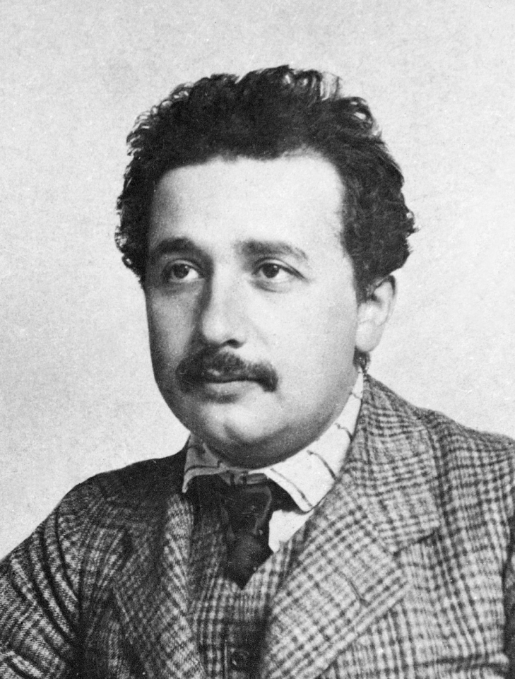
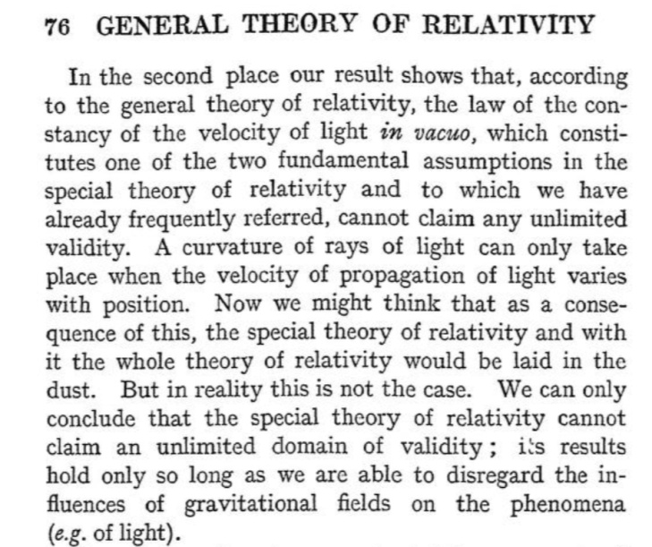
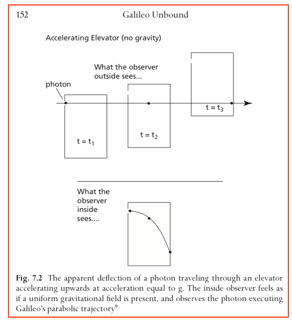
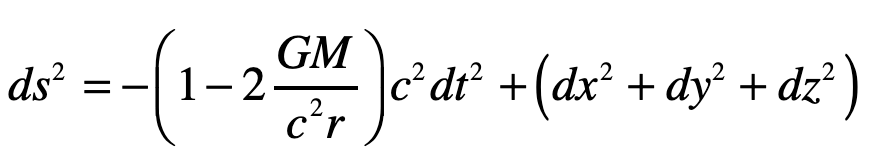
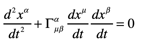
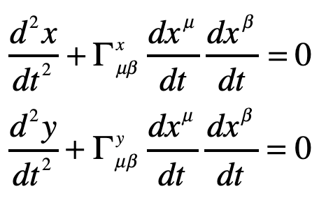
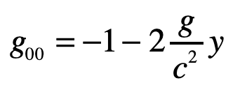
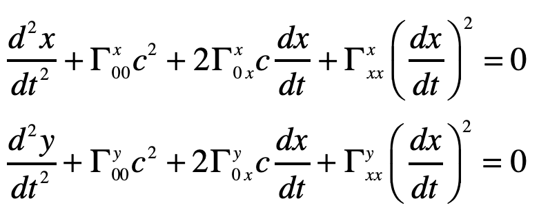
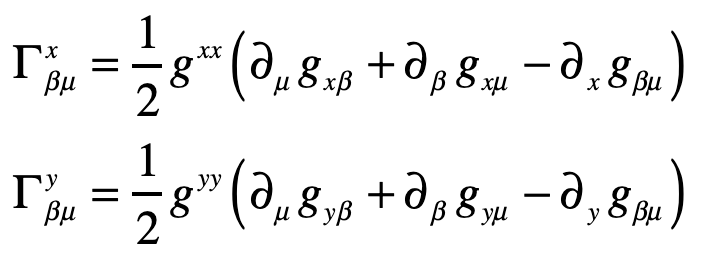
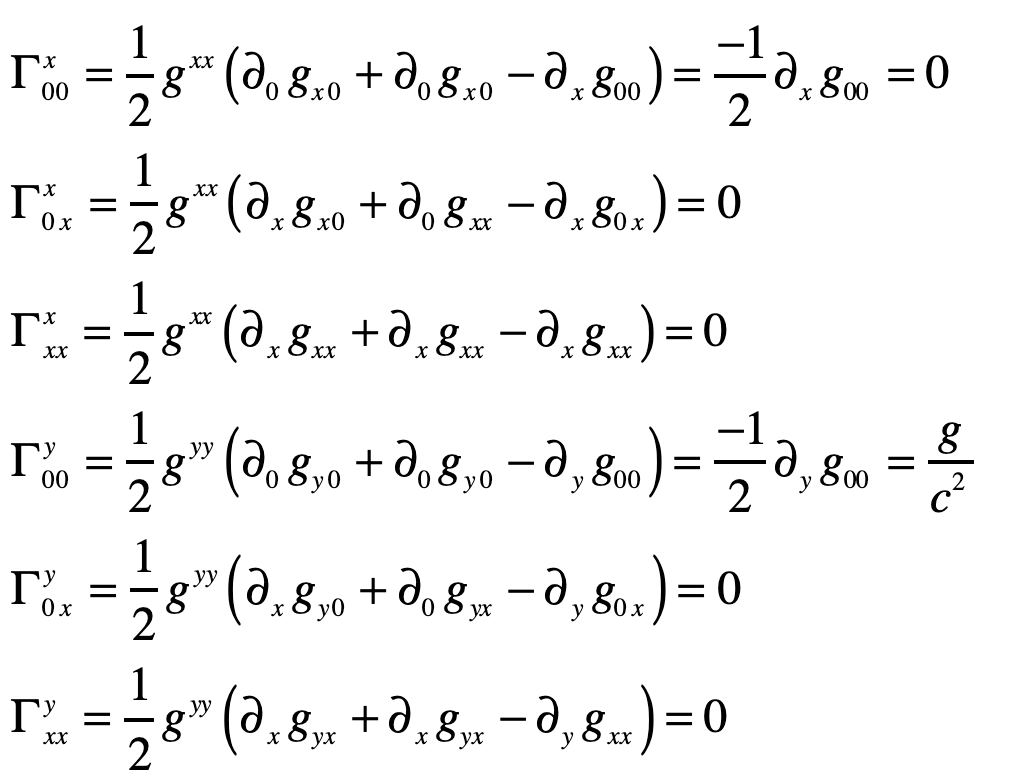
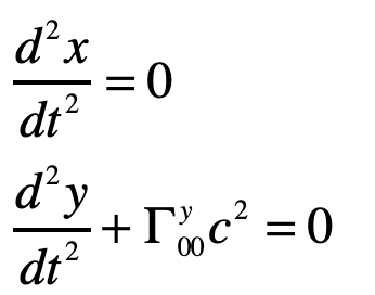
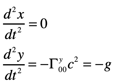
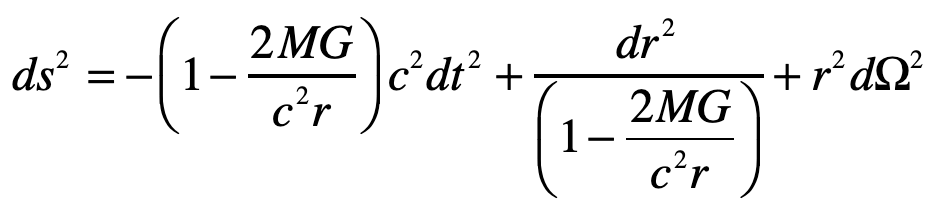
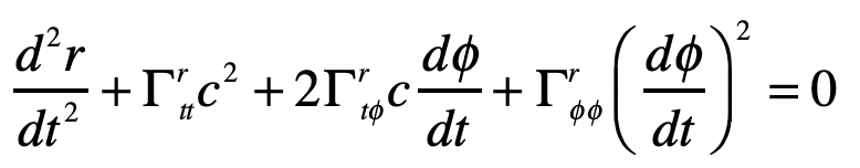
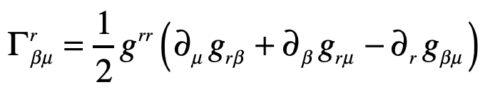
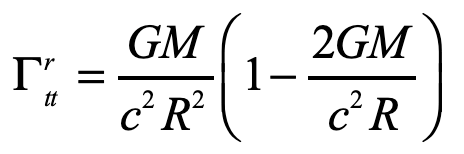
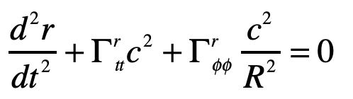
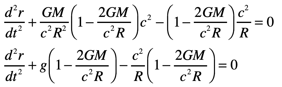
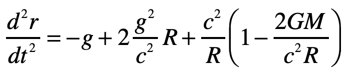
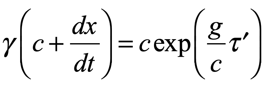
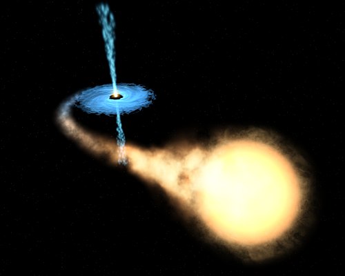
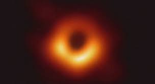
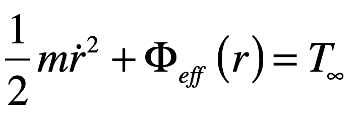
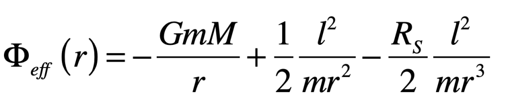
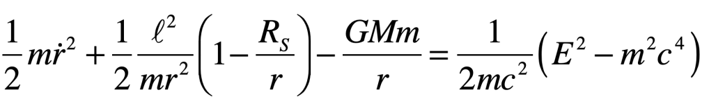
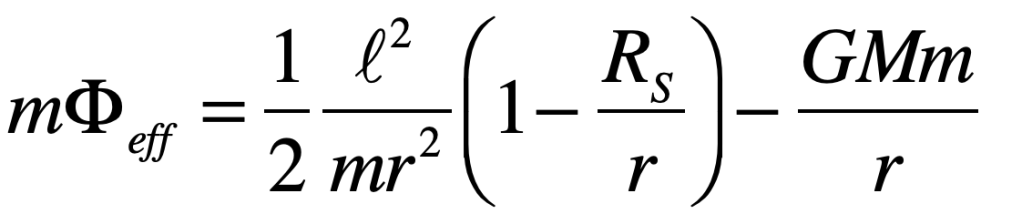
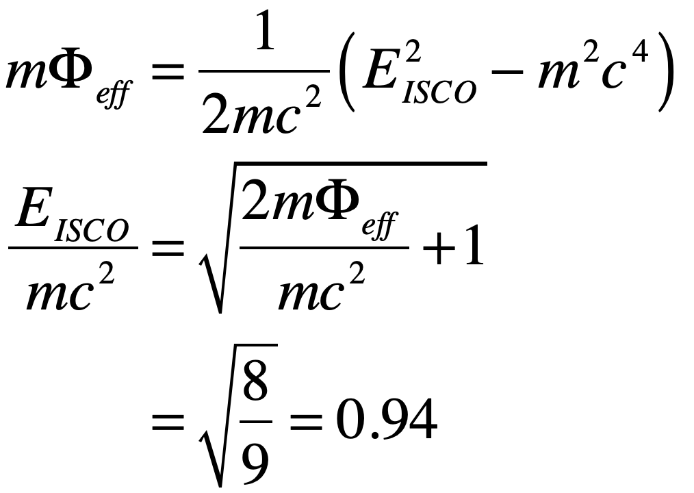
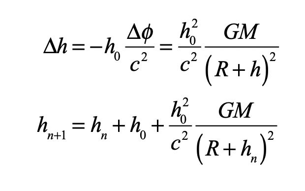
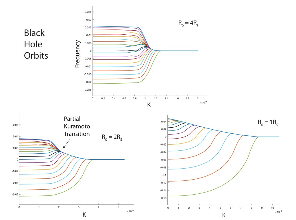
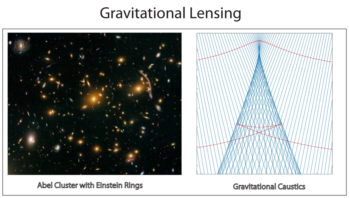
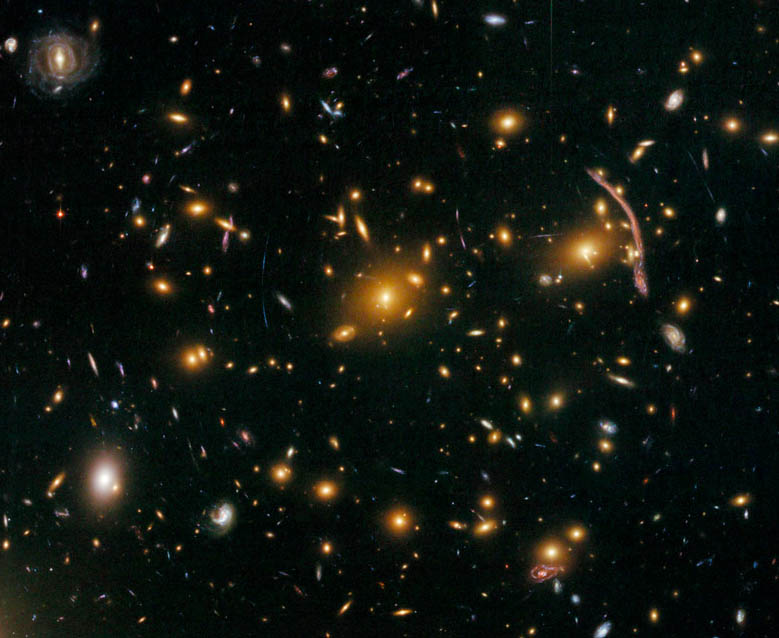
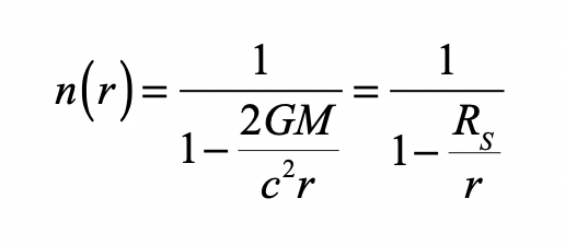
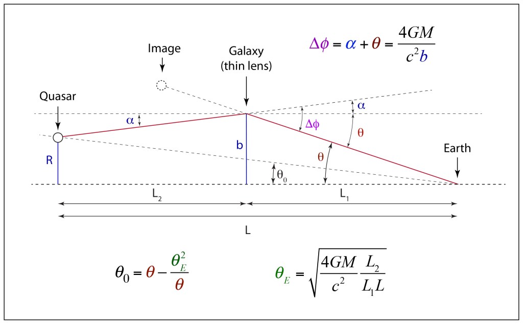
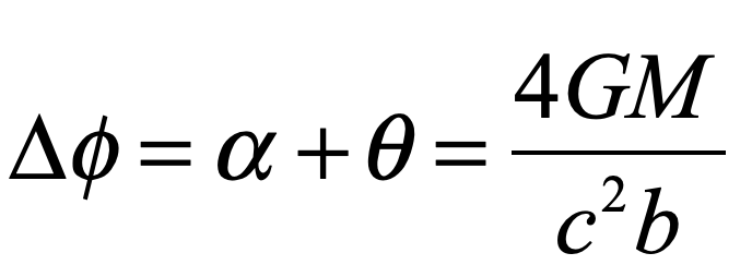
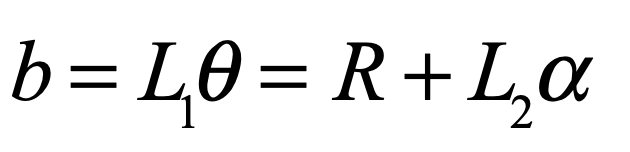
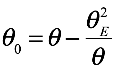
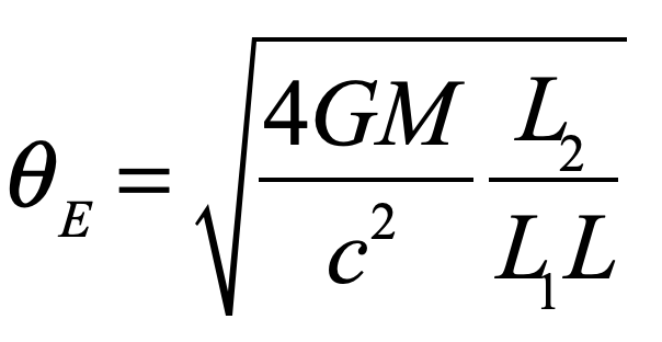
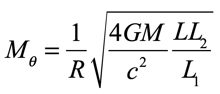
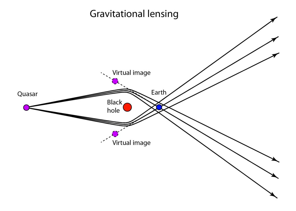
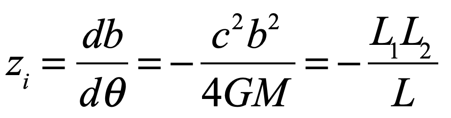
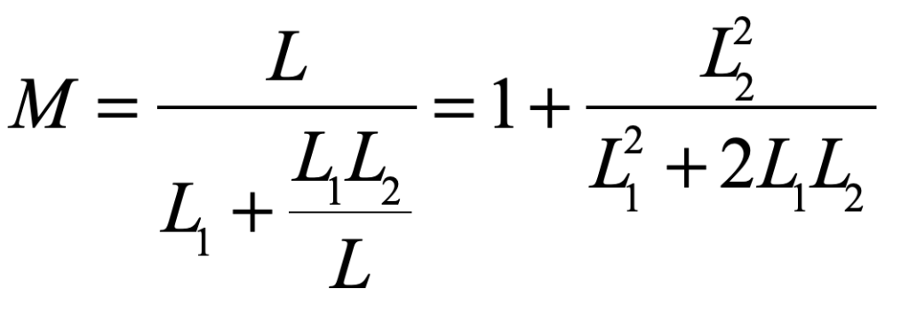
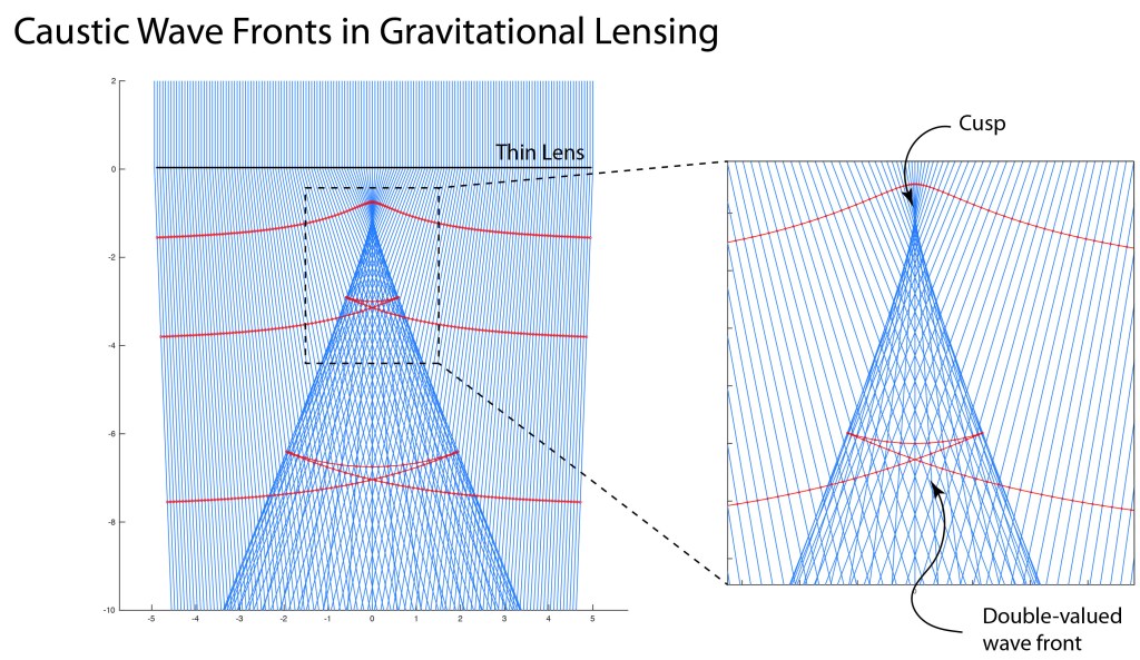
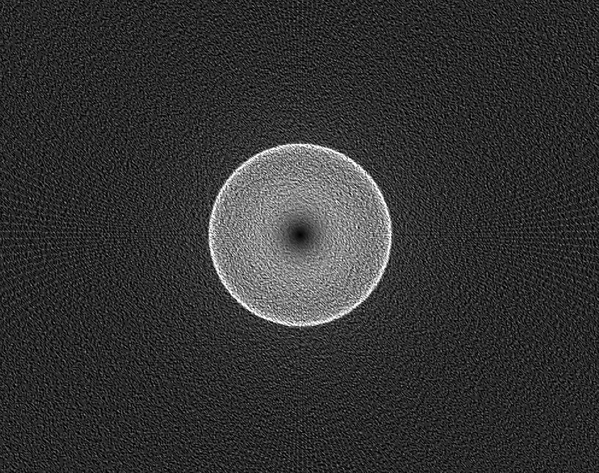
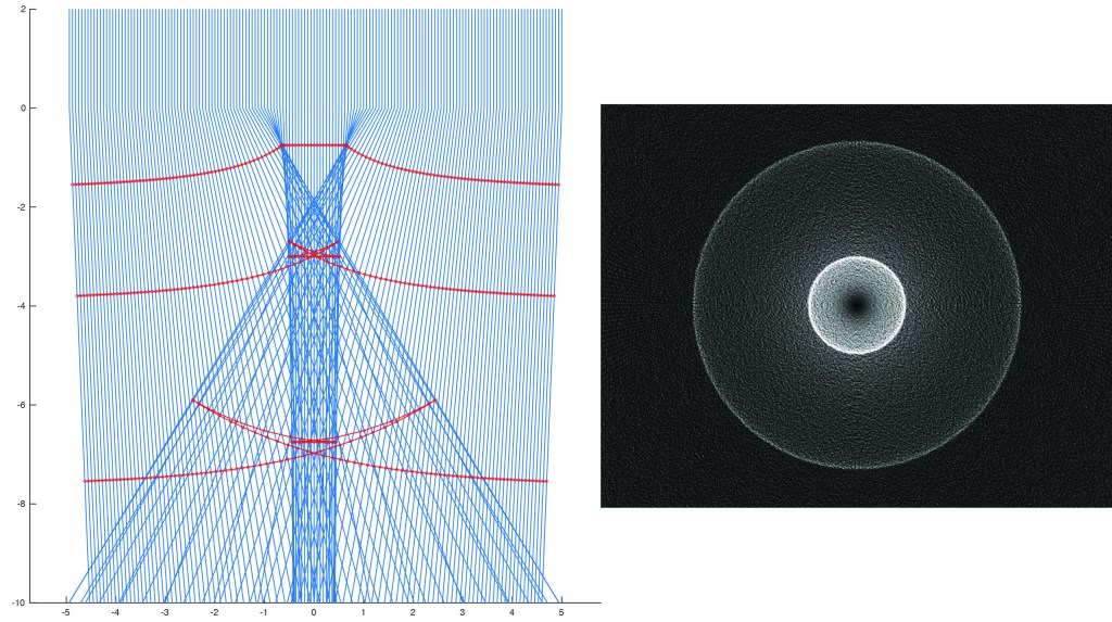
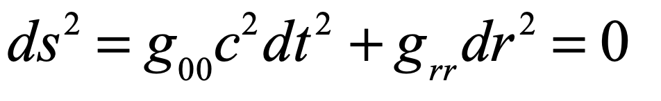
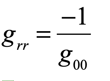
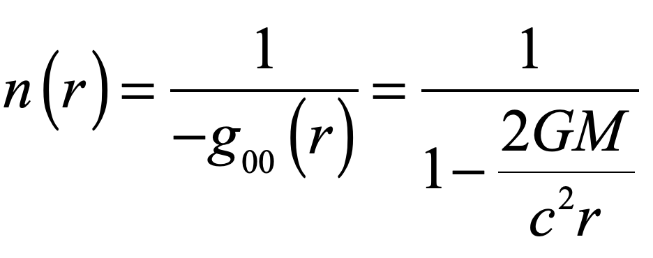
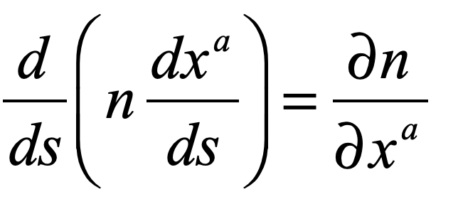
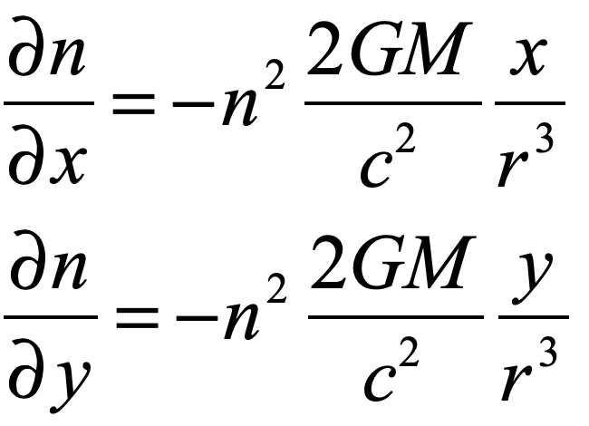
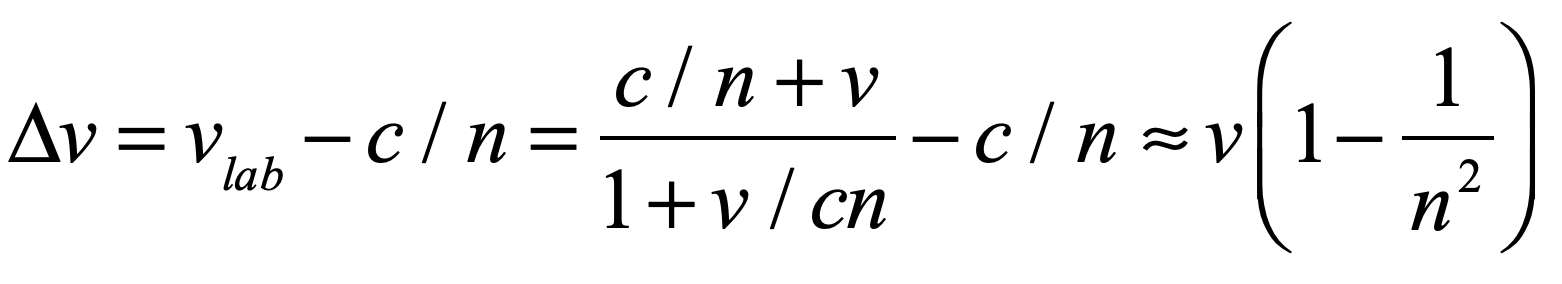
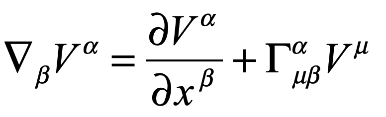
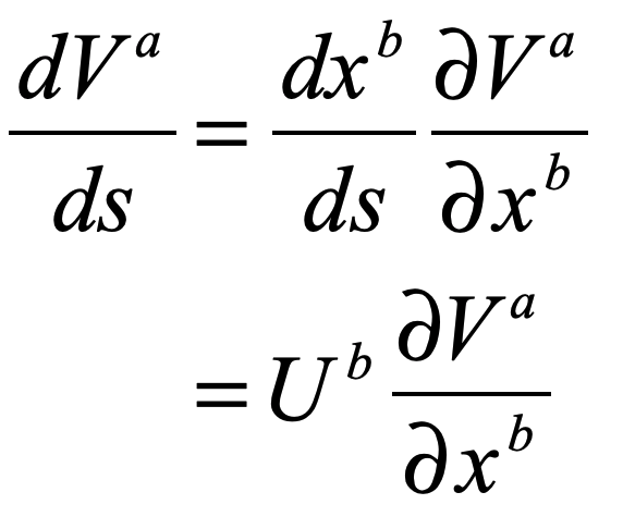
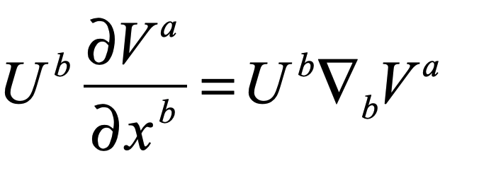
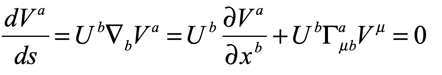
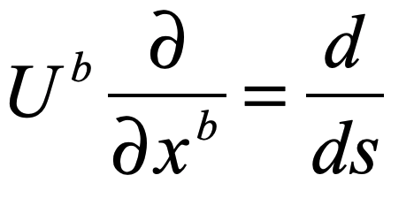
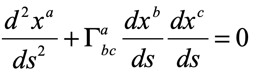
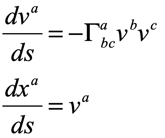
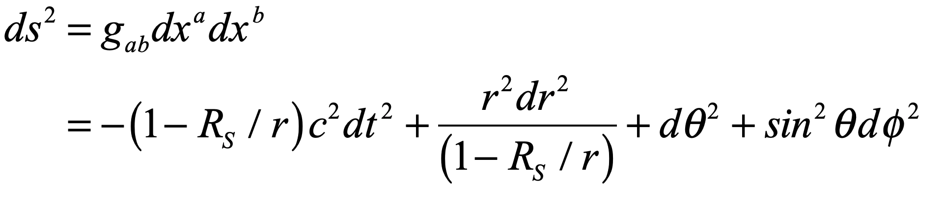
The Lens of Gravity

Gravity provided the backdrop for one of the most important paradigm shifts in the history of physics. Prior to Albert Einstein’s general theory of relativity, trajectories were paths described by geometry. After the theory of general relativity, trajectories are paths caused by geometry. This chapter explains how Einstein arrived at his theory of gravity, relying on the space-time geometry of Hermann Minkowski, whose work he had originally harshly criticized. The confirmation of Einstein’s theory was one of the dramatic high points in 20^th century history of physics when Arthur Eddington journeyed to an island off the coast of Africa to observe stellar deflections during a solar eclipse. If Galileo was the first rock star of physics, then Einstein was the first worldwide rock star of science.

1697 Johann Bernoulli was first to find solution to shortest path between two points on a curved surface (1697).

1728 Euler found the geodesic equation.

1783 The pair 40 Eridani B/C was discovered by William Herschel on 31 January

1783 John Michell explains infalling object would travel faster than speed of light

1796 Laplace describes “dark stars” in Exposition du system du Monde

1827 The first orbit of a binary star computed by Félix Savary for the orbit of Xi Ursae Majoris.

1827 Gauss curvature Theoriem Egregum

1844 Bessel notices periodic displacement of Sirius with period of half a century

1844 The name “geodesic line” is attributed to Liouville.

1845 Buys Ballot used musicians with absolute pitch for the first experimental verification of the Doppler effect

1854 Riemann’s habilitationsschrift

1862 Discovery of Sirius B (a white dwarf)

1868 Darboux suggested motions in n-dimensions

1872 Lipshitz first to apply Riemannian geometry to the principle of least action.

1895 Hilbert arrives in Göttingen

1902 Minkowski arrives in Göttingen

1905 Einstein’s miracle year

1906 Poincaré describes Lorentz transformations as rotations in 4D

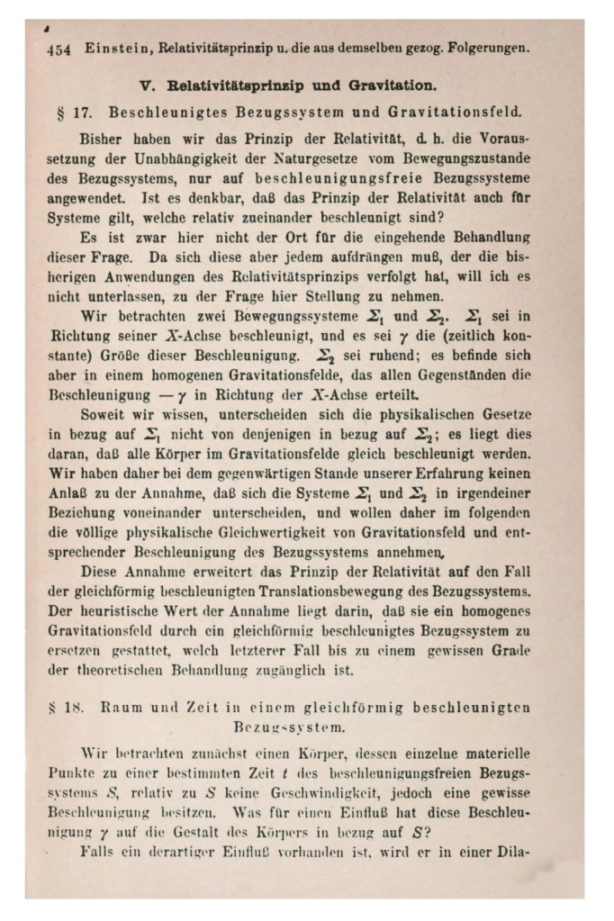
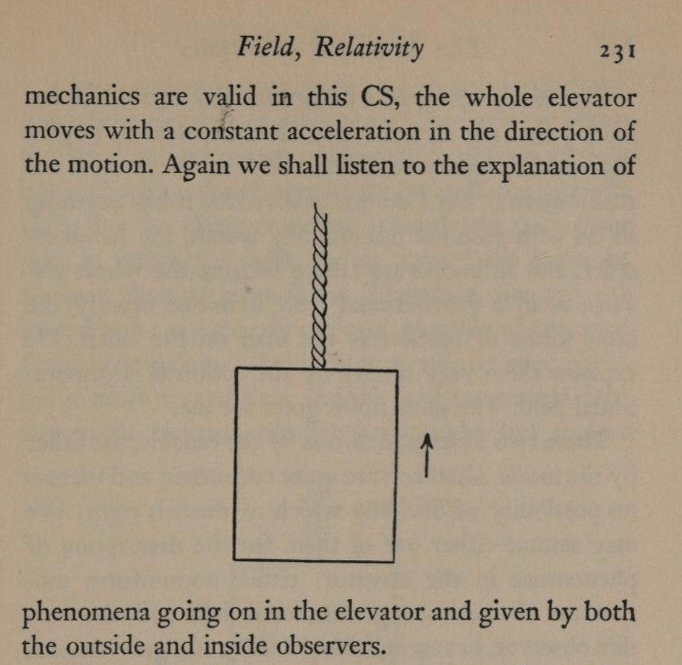
1907 Einstein has “happiest thought” in November

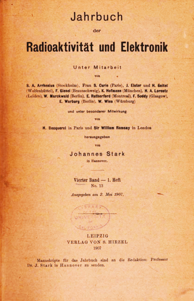
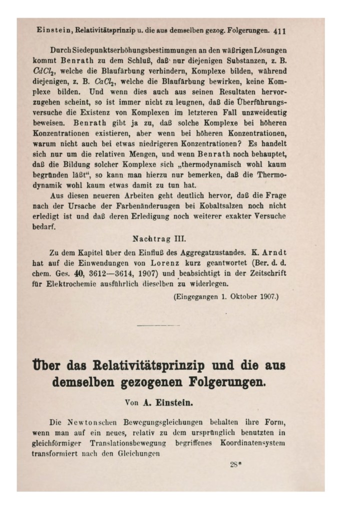
1907 Einstein’s relativity review in Jahrbuch

1908 Minkowski’s Space and Time lecture

1908 Einstein appointed to unpaid position at University of Bern

1909 Minkowski dies

1909 Einstein appointed associate professor of theoretical physics at U of Zürich

1910 40 Eridani B was discobered to be of spectral type A (white dwarf)

1910 Size and mass of Sirius B determined (heavy and small)

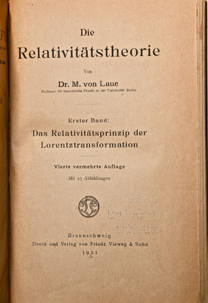
1911 Laue publishes first textbook on relativity theory

1911 Einstein accepts position at Prague

1911 Einstein goes to the limits of special relativity applied to gravitational fields

1912 Einstein’s two papers establish a scalar field theory of gravitation

1912 Einstein moves from Prague to ETH in Zürich in fall. Begins collaboration with Grossmann.

1913 Einstein EG paper

1914 Adams publishes spectrum of 40 Eridani B

1915 Sirius B determined to be also a low-luminosity type A white dwarf

1915 Einstein Completes paper

1916 Density of 40 Eridani B by Ernst Öpik

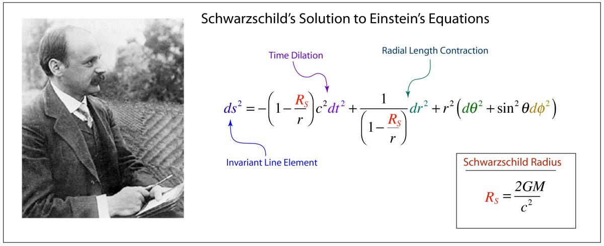
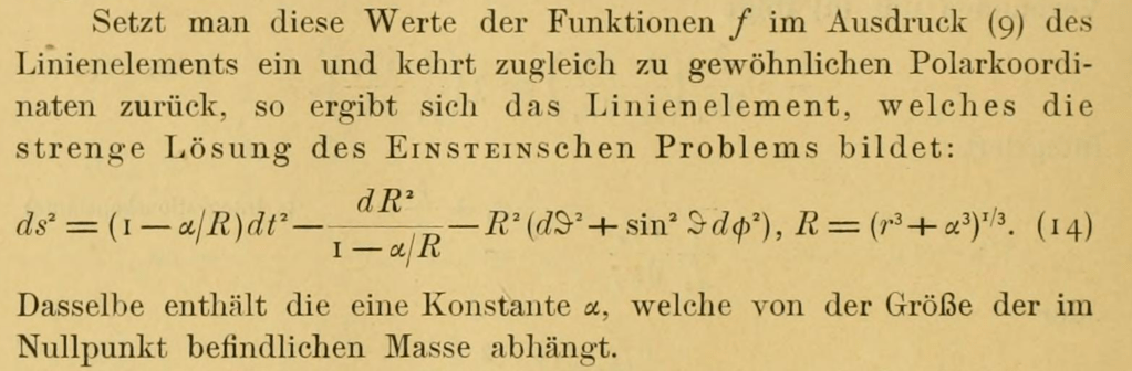
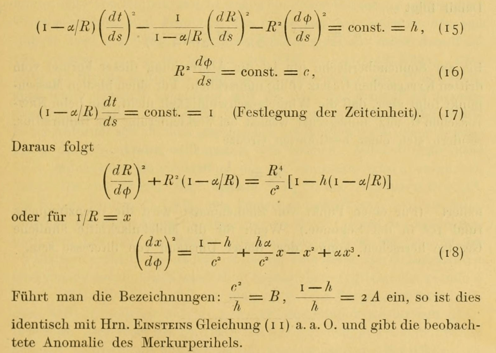
1916 Schwarzschild paper

1916 Einstein’s publishes theory of gravitational waves

1919 Eddington expedition to Principe

1920 Eddington paper on deflection of light by the sun

1922 Willem Luyten coins phrase “white dwarf”

1924 Eddington found a set of coordinates that eliminated the singularity at the Schwarzschild radius

1926 R. H. Fowler publishes paper on degenerate matter and composition of white dwarfs

1931 Chandrasekhar calculated the limit for collapse to white dwarf stars at 1.4MS

1933 Georges Lemaitre states the coordinate singularity was an artefact

1934 Walter Baade and Fritz Zwicky proposed the existence of the neutron star only a year after the discovery of the neutron by Sir James Chadwick.

1939 Oppenheimer and Snyder showed ultimate collapse of a 3M_S “frozen star”

1958 David Finkelstein paper

1965 Antony Hewish and Samuel Okoye discovered “an unusual source of high radio brightness temperature in the Crab Nebula”. This source turned out to be the Crab Nebula neutron star that resulted from the great supernova of 1054.

1967 Jocelyn Bell and Antony Hewish discovered regular radio pulses from CP 1919. This pulsar was later interpreted as an isolated, rotating neutron star.

1967 Wheeler’s “black hole” talk

1974 Joseph Taylor and Russell Hulse discovered the first binary pulsar, PSR B1913+16, which consists of two neutron stars (one seen as a pulsar) orbiting around their center of mass.

2015 LIGO detects gravitational waves on Sept. 14 from the merger of two black holes

2017 LIGO detects the merger of two neutron stars

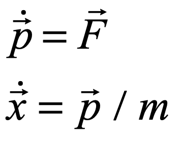
On the Quantum Footpath

The concept of the trajectory of a quantum particle almost vanished in the battle between Werner Heisenberg’s matrix mechanics and Erwin Schrödinger’s wave mechanics. It took Niels Bohr and his complementarity principle of wave-particle duality to cede back some reality to quantum trajectories. However, Schrödinger and Einstein were not convinced and conceived of quantum entanglement to refute the growing acceptance of the Copenhagen Interpretation of quantum physics. Schrödinger’s cat was meant to be an absurdity, but ironically it has become a central paradigm of practical quantum computers. Quantum trajectories took on new meaning when Richard Feynman constructed quantum theory based on the principle of least action, inventing his famous Feynman Diagrams to help explain quantum electrodynamics.

1885 Balmer Theory

1897 J. J. Thomson discovered the electron

1904 Thomson plum pudding model of the atom

1911 Bohr PhD thesis filed. Studies on the electron theory of metals. Visited England.

1911 Rutherford nuclear model

1911 First Solvay conference

1911 “ultraviolet catastrophe” coined by Ehrenfest

1913 Bohr combined Rutherford’s nuclear atom with Planck’s quantum hypothesis: 1913 Bohr model

1913 Ehrenfest adiabatic hypothesis

1914-1916 Bohr at Manchester with Rutherford

1916 Bohr appointed Chair of Theoretical Physics at University of Copenhagen: a position that was made just for him

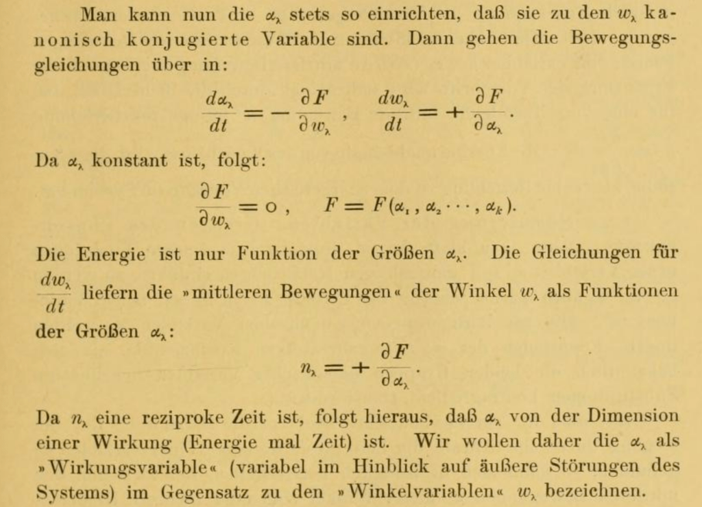
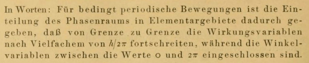
1916 Schwarzschild and Epstein introduce action-angle coordinates into quantum theory

1920 Heisenberg enters University of Munich to obtain his doctorate

1920 Bohr’s Correspondence principle: Classical physics for large quantum numbers

1921 Bohr Founded Institute of Theoretical Physics (Copenhagen)

1922-1923 Heisenberg studies with Born, Franck and Hilbert at Göttingen while Sommerfeld is in the US on sabbatical.

1923 Heisenberg Doctorate. The exam does not go well. Unable to derive the resolving power of a microscope in response to question by Wien. Becomes Born’s assistant at Göttingen.

1924 Heisenberg visits Niels Bohr in Copenhagen (and met Einstein?)

1924 Heisenberg Habilitation at Göttingen on anomalous Zeeman

1924 – 1925 Heisenberg worked with Bohr in Copenhagen, returned summer of 1925 to Göttiingen

1924 Pauli exclusion principle and state occupancy

1924 de Broglie hypothesis extended wave-particle duality to matter

1924 Bohr Predicted Halfnium (72)

1924 Kronig’s proposal for electron self spin

1924 Bose (Einstein)

1925 Heisenberg paper on quantum mechanics

1925 Dirac, reading proof from Heisenberg, recognized the analogy of noncommutativity with Poisson brackets and the correspondence with Hamiltonian mechanics.

1925 Uhlenbeck and Goudschmidt: spin

1926 Born, Heisenberg, Kramers: virtual oscillators at transition frequencies: Matrix mechanics (alternative to Bohr-Kramers-Slater 1924 model of orbits). Heisenberg was Born’s student at Göttingen.

1926 Schrödinger wave mechanics

Schrödinger-1926 Download

1927 de Broglie hypotehsis confirmed by Davisson and Germer

1927 Complementarity by Bohr: wave-particle duality “Evidence obtained under different experimental conditions cannot be comprehended within a single picture, but must be regarded as complementary in the sense that only the totality of the phenomena exhausts the possible information about the objects.”

1927 Heisenberg uncertainty principle (Heisenberg was in Copenhagen 1926 – 1927)

Heisenberg-1927 Download

1927 Solvay Conference in Brussels

1928 Heisenberg to University of Leipzig

1928 Dirac relativistic QM equation

1929 de Broglie Nobel Prize

1930 Solvay Conference

1932 Heisenberg Nobel Prize

1932 von Neumann operator algebra

1933 Dirac Lagrangian form of QM (basis of Feynman path integral)

1933 Schrödinger and Dirac Nobel Prize

1935 Einstein, Poldolsky and Rosen EPR paper

Einstein-1935 Download

1935 Bohr’s response to Einsteins “EPR” paradox

Bohr-1935 Download

1935 Schrodinger’s cat

SchrodingerNW35 Download

SchrodingerNW35-2 Download

SchrodingerNW35-3 Download

1939 Feynman graduates from MIT

1941 Heisenberg (head of German atomic project) visits Bohr in Copenhagen

1942 Feynman PhD at Princeton, “The Principle of Least Action in Quantum Mechanics“

1942 – 1945 Manhattan Project, Bethe-Feynman equation for fission yield

1943 Bohr escapes to Sweden in a fishing boat. Went on to England secretly.

1945 Pauli Nobel Prize

1945 Death of Feynman’s wife Arline (married 4 years)

1945 Fall, Feynman arrives at Cornell ahead of Hans Bethe

1947 Shelter Island conference: Lamb Shift, did Kramer’s give a talk suggesting that infinities could be subtracted?

1947 Fall, Dyson arrives at Cornell

1948 Pocono Manor, Pennsylvania, troubled unveiling of path integral formulation and Feynman diagrams, Schwinger’s master presentation

1948 Feynman and Dirac. Summer drive across the US with Dyson

1949 Dyson joins IAS as a postdoc, trains a cohort of theorists in Feynman’s technique

1949 Karplus and Kroll first g-factor calculation

1950 Feynman moves to Cal Tech

1965 Schwinger, Tomonaga and Feynman Nobel Prize

1967 Hans Bethe Nobel Prize

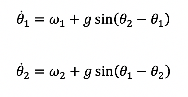
From Butterflies to Hurricanes

Half a century after Poincaré first glimpsed chaos in the three-body problem, the great Russian mathematician Andrey Kolmogorov presented a sketch of a theorem that could prove that orbits are stable. In the hands of Vladimir Arnold and Jürgen Moser, this became the KAM theory of Hamiltonian chaos. This chapter shows how KAM theory fed into topology in the hands of Stephen Smale and helped launch the new field of chaos theory. Edward Lorenz discovered chaos in numerical models of atmospheric weather and discovered the eponymous strange attractor. Mathematical aspects of chaos were further developed by Mitchell Feigenbaum studying bifurcations in the logistic map that describes population dynamics.

1760 Euler 3-body problem (two fixed centers and coplanar third body)

1763 Euler colinear 3-body problem

1772 Lagrange equilateral 3-body problem

1881-1886 Poincare memoires “Sur les courbes de ́finies par une equation differentielle”

1890 Poincare “Sur le probleme des trois corps et les equations de la dynamique”. First-return map, Poincare recurrence theorem, stable and unstable manifolds

1892 – 1899 Poincare New Methods in Celestial Mechanics

1892 Lyapunov The General Problem of the Stability of Motion

1899 Poincare homoclinic trajectory

1913 Birkhoff proves Poincaré’s last geometric theorem, a special case of the three-body problem.

1927 van der Pol and van der Mark

1937 Coarse systems, Andronov and Pontryagin

1938 Morse theory

1942 Hopf bifurcation

1945 Cartwright and Littlewood study the van der Pol equation (Radar during WWII)

1954 Kolmogorov A. N., On conservation of conditionally periodic motions for a small change in Hamilton’s function.

1960 Lorenz: 12 equations

1962 Moser On Invariant Curves of Area-Preserving Mappings of an Annulus.

1963 Arnold Small denominators and problems of the stability of motion in classical and celestial mechanics

1963 Lorenz: 3 equations

1964 Arnold diffusion

1965 Smale’s horseshoe

1969 Chirikov standard map

1971 Ruelle-Takens (Ruelle coins phrase “strange attractor”)

1972 “Butterfly Effect” given for Lorenz’ talk (by Philip Merilees)

1975 Gollub-Swinney observe route to turbulence along lines of Ruelle

1975 Yorke coins “chaos theory”

1976 Robert May writes review article of the logistic map

1977 New York conference on bifurcation theory

1987 James Gleick Chaos: Making a New Science

Darwin in the Clockworks

The preceding timelines related to the central role played by families of trajectories phase space to explain the time evolution of complex systems. These ideas are extended to explore the history and development of the theory of natural evolution by Charles Darwin. Darwin had many influences, including ideas from Thomas Malthus in the context of economic dynamics. After Darwin, the ideas of evolution matured to encompass broad topics in evolutionary dynamics and the emergence of the idea of fitness landscapes and game theory driving the origin of new species. The rise of genetics with Gregor Mendel supplied a firm foundation for molecular evolution, leading to the moleculer clock of Linus Pauling and the replicator dynamics of Richard Dawkins.

1202 Fibonacci

1766 Thomas Robert Malthus born

1776 Adam Smith The Wealth of Nations

1798 Malthus “An Essay on the Principle of Population”

1817 Ricardo Principles of Political Economy and Taxation

1838 Cournot early equilibrium theory in duopoly

1848 John Stuart Mill

1848 Karl Marx Communist Manifesto

1859 Darwin Origin of Species

1867 Karl Marx Das Kapital

1871 Darwin Descent of Man, and Selection in Relation to Sex

1871 Jevons Theory of Political Economy

1871 Menger Principles of Economics

1874 Walrus Éléments d’économie politique pure, or Elements of Pure Economics (1954)

1890 Marshall Principles of Economics

1908 Hardy constant genetic variance

1910 Brouwer fixed point theorem

1910 Alfred J. Lotka autocatylitic chemical reactions

1913 Zermelo determinancy in chess

1922 Fisher dominance ratio

1922 Fisher mutations

1925 Lotka predator-prey in biomathematics

1926 Vita Volterra published same equations independently

1927 JBS Haldane (1892—1964) mutations

1928 von Neumann proves the minimax theorem

1930 Fisher ratio of sexes

1932 Wright Adaptive Landscape

1932 Haldane The Causes of Evolution

1933 Kolmogorov Foundations of the Theory of Probability

1934 Rudolph Carnap The Logical Syntax of Language

1936 John Maynard Keynes, The General Theory of Employment, Interest and Money

1936 Kolmogorov generalized predator-prey systems

1938 Borel symmetric payoff matrix

1942 Sewall Wright Statistical Genetics and Evolution

1943 McCulloch and Pitts A Logical Calculus of Ideas Immanent in Nervous Activity

1944 von Neumann and Morgenstern Theory of Games and Economic Behavior

1950 Prisoner’s Dilemma simulated at Rand Corportation

1950 John Nash Equilibrium points in n-person games and The Bargaining Problem

1951 John Nash Non-cooperative Games

1952 McKinsey Introduction to the Theory of Games (first textbook)

1953 John Nash Two-Person Cooperative Games

1953 Watson and Crick DNA

1955 Braithwaite’s Theory of Games as a Tool for the Moral Philosopher

1961 Lewontin Evolution and the Theory of Games

1962 Patrick Moran The Statistical Processes of Evolutionary Theory

1962 Linus Pauling molecular clock

1968 Motoo Kimura neutral theory of molecular evolution

1972 Maynard Smith introduces the evolutionary stable solution (ESS)

1972 Gould and Eldridge Punctuated equilibrium

1973 Maynard Smith and Price The Logic of Animal Conflict

1973 Black Scholes

1977 Eigen and Schuster The Hypercycle

1978 Replicator equation (Taylor and Jonker)

1982 Hopfield network

1982 John Maynard Smith Evolution and the Theory of Games

1984 R. Axelrod The Evolution of Cooperation

The Measure of Life

This final topic extends the ideas of dynamics into abstract spaces of high dimension to encompass the idea of a trajectory of life. Health and disease become dynamical systems defined by all the proteins and nucleic acids that comprise the physical self. Concepts from network theory, autonomous oscillators and synchronization contribute to this viewpoint. Healthy trajectories are like stable limit cycles in phase space, but disease can knock the system trajectory into dangerous regions of health space, as doctors turn to new developments in personalized medicine try to return the individual to a healthy path. This is the ultimate generalization of Galileo’s simple parabolic trajectory.

1642 Galileo dies

1656 Huygens invents pendulum clock

1665 Huygens observes “odd kind of sympathy” in synchronized clocks

1673 Huygens publishes Horologium Oscillatorium sive de motu pendulorum

1736 Euler Seven Bridges of Königsberg

Euler-Sevenbridges Download

1845 Kirchhoff’s circuit laws

1852 Guthrie four color problem

1857 Cayley trees

1858 Hamiltonian cycles

1887 Cajal neural staining microscopy

1913 Michaelis Menten dynamics of enzymes

1924 Berger, Hans: neural oscillations (Berger invented the EEG)

1926 van der Pol dimensioness form of equation

1927 van der Pol periodic forcing

1943 McCulloch and Pits mathematical model of neural nets

1948 Wiener cybernetics

1952 Hodgkin and Huxley action potential model

1952 Turing instability model

1956 Sutherland cyclic AMP

1957 Broadbent and Hammersley bond percolation

1958 Rosenblatt perceptron

1959 Erdös and Renyi random graphs

1962 Cohen EGF discovered

1965 Sebeok coined zoosemiotics

1966 Mesarovich systems biology

1967 Winfree biological rythms and coupled oscillators

1969 Glass Moire patterns in perception

1970 Rodbell G-protein

1971 phrase “strange attractor” coined (Ruelle)

1972 phrase “signal transduction” coined (Rensing)

1975 phrase “chaos theory” coined (Yorke)

1975 Werbos backpropagation

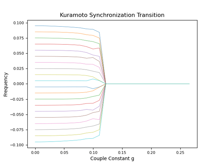
1975 Kuramoto transition

1976 Robert May logistic map

1977 Mackey-Glass equation and dynamical disease

1982 Hopfield network

1990 Strogatz and Murillo pulse-coupled oscillators

1997 Tomita systems biology of a cell

1998 Strogatz and Watts Small World network

1999 Barabasi Scale Free networks

2000 Sequencing of the human genome

The Physics of Life, the Universe and Everything:

Karl Schwarzschild’s Radius: How Fame Eclipsed a Physicist’s own Legacy

In an ironic twist of the history of physics, Karl Schwarzschild’s fame has eclipsed his own legacy. When asked who was Karl Schwarzschild (1873 – 1916), you would probably say he’s the guy who solved Einstein’s Field Equations of General Relativity and discovered the radius of black holes. You may also know that he accomplished this Herculean feat while dying slowly behind the German lines on the Eastern Front in WWI. But asked what else he did, and you would probably come up blank. Yet Schwarzschild was one of the most wide-ranging physicists at the turn of the 20^th century, which is saying something, because it places him into the same pantheon as Planck, Lorentz, Poincaré and Einstein. Let’s take a look at the part of his career that hides in the shadow of his own radius.

A Radius of Interest

Karl Schwarzschild was born in Frankfurt, Germany, shortly after the Franco-Prussian war thrust Prussia onto the world stage as a major political force in Europe. His family were Jewish merchants of longstanding reputation in the city, and Schwarzschild’s childhood was spent in the vibrant Jewish community. One of his father’s friends was a professor at a university in Frankfurt, whose son, Paul Epstein (1871 – 1939), became a close friend of Karl’s at the Gymnasium. Schwarzshild and Epstein would partially shadow each other’s careers despite the fact that Schwarzschild became an astronomer while Epstein became a famous mathematician and number theorist. This was in part because Schwarzschild had large radius of interests that spanned the breadth of current mathematics and science, practicing both experiments and theory.

Schwarzschild’s application of the Hamiltonian formalism for quantum systems set the stage for the later adoption of Hamiltonian methods in quantum mechanics. He came dangerously close to stating the uncertainty principle that catapulted Heisenberg to fame.

By the time Schwarzschild was sixteen, he had taught himself the mathematics of celestial mechanics to such depth that he published two papers on the orbits of binary stars. He also became fascinated in astronomy and purchased lenses and other materials to construct his own telescope. His interests were helped along by Epstein, two years older and whose father had his own private observatory. When Epstein went to study at the University of Strasbourg (then part of the German Federation) Schwarzschild followed him. But Schwarzschild’s main interest in astronomy diverged from Epstein’s main interest in mathematics, and Schwarzschild transferred to the University of Munich where he studied under Hugo von Seeliger (1849 – 1924), the premier German astronomer of his day. Epstein remained at Strasbourg where he studied under Bruno Christoffel (1829 – 1900) and eventually became a professor, but he was forced to relinquish the post when Strasbourg was ceded to France after WWI.

The Birth of Stellar Interferometry

Until the Hubble space telescope was launched in 1990 no star had ever been resolved as a direct image. Within a year of its launch, using its spectacular resolving power, the Hubble optics resolved—just barely—the red supergiant Betelgeuse. No other star (other than the Sun) is close enough or big enough to image the stellar disk, even for the Hubble far above our atmosphere. The reason is that the diameter of the optical lenses and mirrors of the Hubble—as big as they are at 2.4 meter diameter—still produce a diffraction pattern that smears the image so that stars cannot be resolved. Yet information on the size of a distant object is encoded as phase in the light waves that are emitted from the object, and this phase information is accessible to interferometry.

The first physicist who truly grasped the power of optical interferometry and who understood how to design the first interferometric metrology systems was the French physicist Armand Hippolyte Louis Fizeau (1819 – 1896). Fizeau became interested in the properties of light when he collaborated with his friend Léon Foucault (1819–1868) on early uses of photography. The two then embarked on a measurement of the speed of light but had a falling out before the experiment could be finished, and both continued the pursuit independently. Fizeau achieved the first measurement using a toothed wheel rotating rapidly [1], while Foucault came in second using a more versatile system with a spinning mirror [2]. Yet Fizeau surpassed Foucault in optical design and became an expert in interference effects. Interference apparatus had been developed earlier by Augustin Fresnel (the Fresnel bi-prism 1819), Humphrey Lloyd (Lloyd’s mirror 1834) and Jules Jamin (Jamin’s interferential refractor 1856). They had found ways of redirecting light using refraction and reflection to cause interference fringes. But Fizeau was one of the first to recognize that each emitting region of a light source was coherent with itself, and he used this insight and the use of lenses to design the first interferometer.

Fizeau’s interferometer used a lens with a with a tight focal spot masked off by an opaque screen with two open slits. When the masked lens device was focused on an intense light source it produced two parallel pencils of light that were mutually coherent but spatially separated. Fizeau used this apparatus to measure the speed of light in moving water in 1859 [3].

Fig. 1 Optical configuration of the source element of the Fizeau refractometer.

The working principle of the Fizeau refractometer is shown in Fig. 1. The light source is at the bottom, and it is reflected by the partially-silvered beam splitter to pass through the lens and the mask containing two slits. (Only the light paths that pass through the double-slit mask on the lens are shown in the figure.) The slits produce two pencils of mutually coherent light that pass through a system (in the famous Fizeau ether drag experiment it was along two tubes of moving water) and are returned through the same slits, and they intersect at the view port where they produce interference fringes. The fringe spacing is set by the separation of the two slits in the mask. The Rayleigh region of the lens defines a region of spatial coherence even for a so-called “incoherent” source. Therefore, this apparatus, by use of the lens, could convert an incoherent light source into a coherent probe to test the refractive index of test materials, which is why it was called a refractometer.

Fizeau became adept at thinking of alternative optical designs of his refractometer and alternative applications. In an address to the French Physical Society in 1868 he suggested that the double-slit mask could be used on a telescope to determine sizes of distant astronomical objects [4]. There were several subsequent attempts to use Fizeau’s configuration in astronomical observations, but none were conclusive and hence were not widely known.

An optical configuration and astronomical application that was very similar to Fizeau’s idea was proposed by Albert Michelson in 1890 [5]. He built the apparatus and used it to successfully measure the size of several moons of Jupiter [6]. The configuration of the Michelson stellar interferometer is shown in Fig. 2. Light from a distant star passes through two slits in the mask in front of the collecting optics of a telescope. When the two pencils of light intersect at the view port, they produce interference fringes. Because of the finite size of the stellar source, the fringes are partially washed out. By adjusting the slit separation, a certain separation can be found where the fringes completely wash out. The size of the star is then related to the separation of the slits for which the fringe visibility vanishes. This simple principle allows this type of stellar interferometry to measure the size of stars that are large and relatively close to Earth. However, if stars are too far away even this approach cannot be used to measure their sizes because telescopes aren’t big enough. This limitation is currently being bypassed by the use of long-baseline optical interferometers.

Fig. 2 Optical configuration of the Michelson stellar interferometer. Fringes at the view port are partially washed out by the finite size of the star. By adjusting the slit separation, the fringes can be made to vanish entirely, yielding an equation that can be solved for the size of the star.

One of the open questions in the history of interferometry is whether Michelson was aware of Fizeau’s proposal for the stellar interferometer made in 1868. Michelson was well aware of Fizeau’s published research and acknowledged him as a direct inspiration of his own work in interference effects. But Michelson also was unaware of the undercurrents in the French school of optical interference. When he visited Paris in 1881, he met with many of the leading figures in this school (including Lippmann and Cornu), but there is no mention or any evidence that he met with Fizeau. By this time Fizeau’s wife had passed away, and Fizeau spent most of his time in seclusion at his home outside Paris. Therefore, it is unlikely that he would have been present during Michelson’s visit. Because Michelson viewed Fizeau with such awe and respect, if he had met him, he most certainly would have mentioned it. Therefore, Michelson’s invention of the stellar interferometer can be considered with some confidence to be a case of independent discovery. It is perhaps not surprising that he hit on the same idea that Fizeau had in 1868, because Michelson was one of the few physicists who understood coherence and interference at the same depth as Fizeau.

Schwarzschild’s Stellar Interferometer

The physics of the Michelson stellar interferometer is very similar to the physics of Young’s double slit experiment. The two slits in the aperture mask of the telescope objective act to produce a simple sinusoidal interference pattern at the image plane of the optical system. The size of the stellar diameter is determined by using the wash-out effect of the fringes caused by the finite stellar size. However, it is well known to physicists who work with diffraction gratings that a multiple-slit interference pattern has a much greater resolving power than a simple double slit.

This realization must have hit von Seeliger and Schwarzschild, working together at Munich, when they saw the publication of Michelson’s theoretical analysis of his stellar interferometer in 1890, followed by his use of the apparatus to measure the size of Jupiter’s moons. Schwarzschild and von Seeliger realized that by replacing the double-slit mask with a multiple-slit mask, the widths of the interference maxima would be much narrower. Such a diffraction mask on a telescope would cause a star to produce a multiple set of images on the image plane of the telescope associated with the multiple diffraction orders. More interestingly, if the target were a binary star, the diffraction would produce two sets of diffraction maxima—a double image! If the “finesse” of the grating is high enough, the binary star separation could be resolved as a doublet in the diffraction pattern at the image, and the separation could be measured, giving the angular separation of the two stars of the binary system. Such an approach to the binary separation would be a direct measurement, which was a distinct and clever improvement over the indirect Michelson configuration that required finding the extinction of the fringe visibility.

Schwarzschild enlisted the help of a fine German instrument maker to create a multiple slit system that had an adjustable slit separation. The device is shown in Fig. 3 from Schwarzschild’s 1896 publication on the use of the stellar interferometer to measure the separation of binary stars [7]. The device is ingenious. By rotating the chain around the gear on the right-hand side of the apparatus, the two metal plates with four slits could be raised or lowered, cause the projection onto the objective plane to have variable slit spacings. In the operation of the telescope, the changing height of the slits does not matter, because they are near a conjugate optical plane (the entrance pupil) of the optical system. Using this adjustable multiple slit system, Schwarzschild (and two colleagues he enlisted) made multiple observations of well-known binary star systems, and they calculated the star separations. Several of their published results are shown in Fig. 4.

Fig. 3 Illustration from Schwarzschild’s 1896 paper describing an improvement of the Michelson interferometer for measuring the separation of binary star systems Ref. [7].

Fig. 4 Data page from Schwarzschild’s 1896 paper measuring the angular separation of two well-known binary star systems: gamma Leonis and chsi Ursa Major. Ref. [7]

Schwarzschild’s publication demonstrated one of the very first uses of stellar interferometry—well before Michelson himself used his own configuration to measure the diameter of Betelgeuse in 1920. Schwarzschild’s major achievement was performed before he had received his doctorate, on a topic orthogonal to his dissertation topic. Yet this fact is virtually unknown to the broader physics community outside of astronomy. If he had not become so famous later for his solution of Einstein’s field equations, Schwarzschild nonetheless might have been famous for his early contributions to stellar interferometry. But even this was not the end of his unique contributions to physics.

Adiabatic Physics

As Schwarzschild worked for his doctorate under von Seeliger, his dissertation topic was on new theories by Henri Poincaré (1854 – 1912) on celestial mechanics. Poincaré had made a big splash on the international stage with the publication of his prize-winning memoire in 1890 on the three-body problem. This is the publication where Poincaré first described what would later become known as chaos theory. The memoire was followed by his volumes on “New Methods in Celestial Mechanics” published between 1892 and 1899. Poincaré’s work on celestial mechanics was based on his earlier work on the theory of dynamical systems where he discovered important invariant theorems, such as Liouville’s theorem on the conservation of phase space volume. Schwarzshild applied Poincaré’s theorems to problems in celestial orbits. He took his doctorate in 1896 and received a post at an astronomical observatory outside Vienna.

While at Vienna, Schwarzschild performed his most important sustained contributions to the science of astronomy. Astronomical observations had been dominated for centuries by the human eye, but photographic techniques had been making steady inroads since the time of Hermann Carl Vogel (1841 – 1907) in the 1880’s at the Potsdam observatory. Photographic plates were used primarily to record star positions but were known to be unreliable for recording stellar intensities. Schwarzschild developed a “out-of-focus” technique that blurred the star’s image, while making it larger and easier to measure the density of the exposed and developed photographic emulsions. In this way, Schwarzschild measured the magnitudes of 367 stars. Two of these stars had variable magnitudes that he was able to record and track. Schwarzschild correctly explained the intensity variation caused by steady oscillations in heating and cooling of the stellar atmosphere. This work established the properties of these Cepheid variables which would become some of the most important “standard candles” for the measurement of cosmological distances. Based on the importance of this work, Schwarzschild returned to Munich as a teacher in 1899 and subsequently was appointed in 1901 as the director of the observatory at Göttingen established by Gauss eighty years earlier.

Schwarzschild’s years at Göttingen brought him into contact with some of the greatest mathematicians and physicists of that era. The mathematicians included Felix Klein, David Hilbert and Hermann Minkowski. The physicists included von Laue, a student of Woldemar Voigt. This period was one of several “golden ages” of Göttingen. The first golden age was the time of Gauss and Riemann in the mid-1800’s. The second golden age, when Schwarzschild was present, began when Felix Klein arrived at Göttingen and attracted the top mathematicians of the time. The third golden age of Göttingen was the time of Born and Jordan and Heisenberg at the birth of quantum mechanics in the mid 1920’s.

In 1906, the Austrian Physicist Paul Ehrenfest, freshly out of his PhD under the supervision of Boltzmann, arrived at Göttingen only weeks before Boltzmann took his own life. Felix Klein at Göttingen had been relying on Boltzmann to provide a comprehensive review of statistical mechanics for the Mathematical Encyclopedia, so he now entrusted this project to the young Ehrenfest. It was a monumental task, which was to take him and his physicist wife Tatyanya nearly five years to complete. Part of the delay was the desire by the Ehrenfests to close some open problems that remained in Boltzmann’s work. One of these was a mechanical theorem of Boltzmann’s that identified properties of statistical mechanical systems that remained unaltered through a very slow change in system parameters. These properties would later be called adiabatic invariants by Einstein.

Ehrenfest recognized that Wien’s displacement law, which had been a guiding light for Planck and his theory of black body radiation, had originally been derived by Wien using classical principles related to slow changes in the volume of a cavity. Ehrenfest was struck by the fact that such slow changes would not induce changes in the quantum numbers of the quantized states, and hence that the quantum numbers must be adiabatic invariants of the black body system. This not only explained why Wien’s displacement law continued to hold under quantum as well as classical considerations, but it also explained why Planck’s quantization of the energy of his simple oscillators was the only possible choice. For a classical harmonic oscillator, the ratio of the energy of oscillation to the frequency of oscillation is an adiabatic invariant, which is immediately recognized as Planck’s quantum condition .

Ehrenfest published his observations in 1913 [8], the same year that Bohr published his theory of the hydrogen atom, so Ehrenfest immediately applied the theory of adiabatic invariants to Bohr’s model and discovered that the quantum condition for the quantized energy levels was again the adiabatic invariants of the electron orbits, and not merely a consequence of integer multiples of angular momentum, which had seemed somewhat ad hoc.

After eight exciting years at Göttingen, Schwarzschild was offered the position at the Potsdam Observatory in 1909 upon the retirement from that post of the famous German astronomer Carl Vogel who had made the first confirmed measurements of the optical Doppler effect. Schwarzschild accepted and moved to Potsdam with a new family. His son Martin Schwarzschild would follow him into his profession, becoming a famous astronomer at Princeton University and a theorist on stellar structure. At the outbreak of WWI, Schwarzschild joined the German army out of a sense of patriotism. Because of his advanced education he was made an officer of artillery with the job to calculate artillery trajectories, and after a short time on the Western Front in Belgium was transferred to the Eastern Front in Russia. Though he was not in the trenches, he was in the midst of the chaos to the rear of the front. Despite this situation, he found time to pursue his science through the year 1915.

Schwarzschild was intrigued by Ehrenfest’s paper on adiabatic invariants and their similarity to several of the invariant theorems of Poincaré that he had studied for his doctorate. Up until this time, mechanics had been mostly pursued through the Lagrangian formalism which could easily handle generalized forces associated with dissipation. But celestial mechanics are conservative systems for which the Hamiltonian formalism is a more natural approach. In particular, the Hamilton-Jacobi canonical transformations made it particularly easy to find pairs of generalized coordinates that had simple periodic behavior. In his published paper [9], Schwarzschild called these “Action-Angle” coordinates because one was the action integral that was well-known in the principle of “Least Action”, and the other was like an angle variable that changed steadily in time (see Fig. 5). Action-angle coordinates have come to form the foundation of many of the properties of Hamiltonian chaos, Hamiltonian maps, and Hamiltonian tapestries.

Fig. 5 Description of the canonical transformation to action-angle coordinates (Ref. [9] pg. 549). Schwarzschild names the new coordinates “Wirkungsvariable” and “Winkelvariable”.

During lulls in bombardments, Schwarzschild translated the Hamilton-Jacobi methods of celestial mechanics to apply them to the new quantum mechanics of the Bohr orbits. The phrase “quantum mechanics” had not yet been coined (that would come ten years later in a paper by Max Born), but it was clear that the Bohr quantization conditions were a new type of mechanics. The periodicities that were inherent in the quantum systems were natural properties that could be mapped onto the periodicities of the angle variables, while Ehrenfest’s adiabatic invariants could be mapped onto the slowly varying action integrals. Schwarzschild showed that action-angle coordinates were the only allowed choice of coordinates, because they enabled the separation of the Hamilton-Jacobi equations and hence provided the correct quantization conditions for the Bohr electron orbits. Later, when Sommerfeld published his quantized elliptical orbits in 1916, the multiplicity of quantum conditions and orbits had caused concern, but Ehrenfest came to the rescue, showing that each of Sommerfeld’s quantum conditions were precisely Schwarzschild’s action-integral invariants of the classical electron dynamics [10].

The works by Schwarzschild, and a closely-related paper that amplified his ideas published by his friend Paul Epstein several months later [11], were the first to show the power of the Hamiltonian formulation of dynamics for quantum systems, foreshadowing the future importance of Hamiltonians for quantum theory. An essential part of the Hamiltonian formalism is the concept of phase space. In his paper, Schwarzschild showed that the phase space of quantum systems was divided into small but finite elementary regions whose areas were equal to Planck’s constant h-bar (see Fig. 6). The areas were products of a small change in momentum coordinate Delta-p and a corresponding small change in position coordinate Delta-x. Therefore, the product DxDp = h-bar. This observation, made in 1915 by Schwarzschild, was only one step away from Heisenberg’s uncertainty relation, twelve years before Heisenberg discovered it. However, in 1915 Born’s probabilistic interpretation of quantum mechanics had not yet been made, nor the idea of measurement uncertainty, so Schwarzschild did not have the appropriate context in which to have made the leap to the uncertainty principle. However, by introducing the action-angle coordinates as well as the Hamiltonian formalism applied to quantum systems, with the natural structure of phase space, Schwarzschild laid the foundation for the future developments in quantum theory made by the next generation.

Fig. 6 Expression of the division of phase space into elemental areas of action equal to h-bar (Ref. [9] pg. 550).

All Quiet on the Eastern Front

Towards the end of his second stay in Munich in 1900, prior to joining the Göttingen faculty, Schwarzschild had presented a paper at a meeting of the German Astronomical Society held in Heidelberg in August. The topic was unlike anything he had tackled before. It considered the highly theoretical question of whether the universe was non-Euclidean, and more specifically if it had curvature. He concluded from observation that if the universe were curved, the radius of curvature must be larger than between 50 light years and 2000 light years, depending on whether the geometry was hyperbolic or elliptical. Schwarzschild was working out ideas of differential geometry and applying them to the universe at large at a time when Einstein was just graduating from the ETH where he skipped his math classes and had his friend Marcel Grossmann take notes for him.

The topic of Schwarzschild’s talk tells an important story about the warping of historical perspective by the “great man” syndrome. In this case the great man is Einstein who is today given all the credit for discovering the warping of space. His development of General Relativity is often portrayed as by a lone genius in the wilderness performing a blazing act of creation out of the void. In fact, non-Euclidean geometry had been around for some time by 1900—five years before Einstein’s Special Theory and ten years before his first publications on the General Theory. Gauss had developed the idea of intrinsic curvature of a manifold fifty years earlier, amplified by Riemann. By the turn of the century alternative geometries were all the rage, and Schwarzschild considered whether there were sufficient astronomical observations to set limits on the size of curvature of the universe. But revisionist history is just as prevalent in physics as in any field, and when someone like Einstein becomes so big in the mind’s eye, his shadow makes it difficult to see all the people standing behind him.

This is not meant to take away from the feat that Einstein accomplished. The General Theory of Relativity, published by Einstein in its full form in 1915 was spectacular [12]. Einstein had taken vague notions about curved spaces and had made them specific, mathematically rigorous and intimately connected with physics through the mass-energy source term in his field equations. His mathematics had gone beyond even what his mathematician friend and former collaborator Grossmann could achieve. Yet Einstein’s field equations were nonlinear tensor differential equations in which the warping of space depended on the strength of energy fields, but the configuration of those energy fields depended on the warping of space. This type of nonlinear equation is difficult to solve in general terms, and Einstein was not immediately aware of how to find the solutions to his own equations.

Therefore, it was no small surprise to him when he received a letter from the Eastern Front from an astronomer he barely knew who had found a solution—a simple solution (see Fig. 7) —to his field equations. Einstein probably wondered how he could have missed it, but he was generous and forwarded the letter to the Reports of the Prussian Physical Society where it was published in 1916 [13].

Fig. 7 Schwarzschild’s solution of the Einstein Field Equations (Ref. [13] pg. 194).

In the same paper, Schwarzschild used his exact solution to find the exact equation that described the precession of the perihelion of Mercury that Einstein had only calculated approximately. The dynamical equations for Mercury are shown in Fig. 8.

Fig. 8 Explanation for the precession of the perihelion of Mercury ( Ref. [13] pg. 195)

Schwarzschild’s solution to Einstein’s Field Equation of General Relativity was not a general solution, even for a point mass. He had constants of integration that could have arbitrary values, such as the characteristic length scale that Schwarzschild called “alpha”. It was David Hilbert who later expanded upon Schwarzschild’s work, giving the general solution and naming the characteristic length scale (where the metric diverges) after Schwarzschild. This is where the phrase “Schwarzschild Radius” got its name, and it stuck. In fact it stuck so well that Schwarzschild’s radius has now eclipsed much of the rest of Schwarzschild’s considerable accomplishments.

Unfortunately, Schwarzschild’s accomplishments were cut short when he contracted an autoimmune disease that may have been hereditary. It is ironic that in the carnage of the Eastern Front, it was a genetic disease that caused his death at the age of 42. He was already suffering from the effects of the disease as he worked on his last publications. He was sent home from the front to his family in Potsdam where he passed away several months later having shepherded his final two papers through the publication process. His last paper, on the action-angle variables in quantum systems , was published on the day that he died.

Schwarzschild’s Legacy

Schwarzschild’s legacy was assured when he solved Einstein’s field equations and Einstein communicated it to the world. But his hidden legacy is no less important.

Schwarzschild’s application of the Hamiltonian formalism of canonical transformations and phase space for quantum systems set the stage for the later adoption of Hamiltonian methods in quantum mechanics. He came dangerously close to stating the uncertainty principle that catapulted Heisenberg to later fame, although he could not express it in probabilistic terms because he came too early.

Schwarzschild is considered to be the greatest German astronomer of the last hundred years. This is in part based on his work at the birth of stellar interferometry and in part on his development of stellar photometry and the calibration of the Cepheid variable stars that went on to revolutionize our view of our place in the universe. Solving Einsteins field equations was just a sideline for him, a hobby to occupy his active and curious mind.

The Physics of Life, the Universe and Everyting:

References

[1] Fizeau, H. L. (1849). “Sur une expérience relative à la vitesse de propagation de la lumière.” Comptes rendus de l’Académie des sciences 29: 90–92, 132.

[2] Foucault, J. L. (1862). “Détermination expérimentale de la vitesse de la lumière: parallaxe du Soleil.” Comptes rendus de l’Académie des sciences 55: 501–503, 792–596.

[3] Fizeau, H. (1859). “Sur les hypothèses relatives à l’éther lumineux.” Ann. Chim. Phys. Ser. 4 57: 385–404.

[4] Fizeau, H. (1868). “Prix Bordin: Rapport sur le concours de l’annee 1867.” C. R. Acad. Sci. 66: 932.

[5] Michelson, A. A. (1890). “I. On the application of interference methods to astronomical measurements.” The London, Edinburgh, and Dublin Philosophical Magazine and Journal of Science 30(182): 1-21.

[6] Michelson, A. A. (1891). “Measurement of Jupiter’s Satellites by Interference.” Nature 45(1155): 160-161.

[7] Schwarzschild, K. (1896). “Über messung von doppelsternen durch interferenzen.” Astron. Nachr. 3335: 139.

[8] P. Ehrenfest, “Een mechanische theorema van Boltzmann en zijne betrekking tot de quanta theorie (A mechanical theorem of Boltzmann and its relation to the theory of energy quanta),” Verslag van de Gewoge Vergaderingen der Wis-en Natuurkungige Afdeeling, vol. 22, pp. 586-593, 1913.

[9] Schwarzschild, K. (1916). “Quantum hypothesis.” Sitzungsberichte Der Koniglich Preussischen Akademie Der Wissenschaften: 548-568.

[10] P. Ehrenfest, “Adiabatic invariables and quantum theory,” Annalen Der Physik, vol. 51, pp. 327-352, Oct 1916.

[11] Epstein, P. S. (1916). “The quantum theory.” Annalen Der Physik 51(18): 168-188.

[12] Einstein, A. (1915). “On the general theory of relativity.” Sitzungsberichte Der Koniglich Preussischen Akademie Der Wissenschaften: 778-786.

[13] Schwarzschild, K. (1916). “Über das Gravitationsfeld eines Massenpunktes nach der Einstein’schen Theorie.” Sitzungsberichte der Königlich-Preussischen Akademie der Wissenschaften: 189.

July 29, 2019October 24, 2023 by David D. Nolte

Orbiting Photons around a Black Hole

The physics of a path of light passing a gravitating body is one of the hardest concepts to understand in General Relativity, but it is also one of the easiest. It is hard because there can be no force of gravity on light even though the path of a photon bends as it passes a gravitating body. It is easy, because the photon is following the simplest possible path—a geodesic equation for force-free motion.

This blog picks up where my last blog left off, having there defined the geodesic equation and presenting the Schwarzschild metric. With those two equations in hand, we could simply solve for the null geodesics (a null geodesic is the path of a light beam through a manifold). But there turns out to be a simpler approach that Einstein came up with himself (he never did like doing things the hard way). He just had to sacrifice the fundamental postulate that he used to explain everything about Special Relativity.

Throwing Special Relativity Under the Bus

The fundamental postulate of Special Relativity states that the speed of light is the same for all observers. Einstein posed this postulate, then used it to derive some of the most astonishing consequences of Special Relativity—like E = mc². This postulate is at the rock core of his theory of relativity and can be viewed as one of the simplest “truths” of our reality—or at least of our spacetime.

Yet as soon as Einstein began thinking how to extend SR to a more general situation, he realized almost immediately that he would have to throw this postulate out. While the speed of light measured locally is always equal to c, the apparent speed of light observed by a distant observer (far from the gravitating body) is modified by gravitational time dilation and length contraction. This means that the apparent speed of light, as observed at a distance, varies as a function of position. From this simple conclusion Einstein derived a first estimate of the deflection of light by the Sun, though he initially was off by a factor of 2. (The full story of Einstein’s derivation of the deflection of light by the Sun and the confirmation by Eddington is in Chapter 7 of Galileo Unbound (Oxford University Press, 2018).)

The “Optics” of Gravity

The invariant element for a light path moving radially in the Schwarzschild geometry is

The apparent speed of light is then

where c(r) is always less than c, when observing it from flat space. The “refractive index” of space is defined, as for any optical material, as the ratio of the constant speed divided by the observed speed

Because the Schwarzschild metric has the property

the effective refractive index of warped space-time is

with a divergence at the Schwarzschild radius.

The refractive index of warped space-time in the limit of weak gravity can be used in the ray equation (also known as the Eikonal equation described in an earlier blog)

where the gradient of the refractive index of space is

The ray equation is then a four-variable flow

These equations represent a 4-dimensional flow for a light ray confined to a plane. The trajectory of any light path is found by using an ODE solver subject to the initial conditions for the direction of the light ray. This is simple for us to do today with Python or Matlab, but it was also that could be done long before the advent of computers by early theorists of relativity like Max von Laue (1879 – 1960).

The Relativity of Max von Laue

In the Fall of 1905 in Berlin, a young German physicist by the name of Max Laue was sitting in the physics colloquium at the University listening to another Max, his doctoral supervisor Max Planck, deliver a seminar on Einstein’s new theory of relativity. Laue was struck by the simplicity of the theory, in this sense “simplistic” and hence hard to believe, but the beauty of the theory stuck with him, and he began to think through the consequences for experiments like the Fizeau experiment on partial ether drag.

Armand Hippolyte Louis Fizeau (1819 – 1896) in 1851 built one of the world’s first optical interferometers and used it to measure the speed of light inside moving fluids. At that time the speed of light was believed to be a property of the luminiferous ether, and there were several opposing theories on how light would travel inside moving matter. One theory would have the ether fully stationary, unaffected by moving matter, and hence the speed of light would be unaffected by motion. An opposite theory would have the ether fully entrained by matter and hence the speed of light in moving matter would be a simple sum of speeds. A middle theory considered that only part of the ether was dragged along with the moving matter. This was Fresnel’s partial ether drag hypothesis that he had arrived at to explain why his friend Francois Arago had not observed any contribution to stellar aberration from the motion of the Earth through the ether. When Fizeau performed his experiment, the results agreed closely with Fresnel’s drag coefficient, which seemed to settle the matter. Yet when Michelson and Morley performed their experiments of 1887, there was no evidence for partial drag.

Even after the exposition by Einstein on relativity in 1905, the disagreement of the Michelson-Morley results with Fizeau’s results was not fully reconciled until Laue showed in 1907 that the velocity addition theorem of relativity gave complete agreement with the Fizeau experiment. The velocity observed in the lab frame is found using the velocity addition theorem of special relativity. For the Fizeau experiment, water with a refractive index of n is moving with a speed v and hence the speed in the lab frame is

The difference in the speed of light between the stationary and the moving water is the difference

where the last term is precisely the Fresnel drag coefficient. This was one of the first definitive “proofs” of the validity of Einstein’s theory of relativity, and it made Laue one of relativity’s staunchest proponents. Spurred on by his success with the Fresnel drag coefficient explanation, Laue wrote the first monograph on relativity theory, publishing it in 1910.

Fig. 1 Front page of von Laue’s textbook, first published in 1910, on Special Relativity (this is a 4-th edition published in 1921).

A Nobel Prize for Crystal X-ray Diffraction

In 1909 Laue became a Privatdozent under Arnold Sommerfeld (1868 – 1951) at the university in Munich. In the Spring of 1912 he was walking in the Englischer Garten on the northern edge of the city talking with Paul Ewald (1888 – 1985) who was finishing his doctorate with Sommerfed studying the structure of crystals. Ewald was considering the interaction of optical wavelength with the periodic lattice when it struck Laue that x-rays would have the kind of short wavelengths that would allow the crystal to act as a diffraction grating to produce multiple diffraction orders. Within a few weeks of that discussion, two of Sommerfeld’s students (Friedrich and Knipping) used an x-ray source and photographic film to look for the predicted diffraction spots from a copper sulfate crystal. When the film was developed, it showed a constellation of dark spots for each of the diffraction orders of the x-rays scattered from the multiple periodicities of the crystal lattice. Two years later, in 1914, Laue was awarded the Nobel prize in physics for the discovery. That same year his father was elevated to the hereditary nobility in the Prussian empire and Max Laue became Max von Laue.

Von Laue was not one to take risks, and he remained conservative in many of his interests. He was immensely respected and played important roles in the administration of German science, but his scientific contributions after receiving the Nobel Prize were only modest. Yet as the Nazis came to power in the early 1930’s, he was one of the few physicists to stand up and resist the Nazi take-over of German physics. He was especially disturbed by the plight of the Jewish physicists. In 1933 he was invited to give the keynote address at the conference of the German Physical Society in Wurzburg where he spoke out against the Nazi rejection of relativity as they branded it “Jewish science”. In his speech he likened Einstein, the target of much of the propaganda, to Galileo. He said, “No matter how great the repression, the representative of science can stand erect in the triumphant certainty that is expressed in the simple phrase: And yet it moves.” Von Laue believed that truth would hold out in the face of the proscription against relativity theory by the Nazi regime. The quote “And yet it moves” is supposed to have been muttered by Galileo just after his abjuration before the Inquisition, referring to the Earth moving around the Sun. Although the quote is famous, it is believed to be a myth.

In an odd side-note of history, von Laue sent his gold Nobel prize medal to Denmark for its safe keeping with Niels Bohr so that it would not be paraded about by the Nazi regime. Yet when the Nazis invaded Denmark, to avoid having the medals fall into the hands of the Nazis, the medal was dissolved in aqua regia by a member of Bohr’s team, George de Hevesy. The gold completely dissolved into an orange liquid that was stored in a beaker high on a shelf through the war. When Denmark was finally freed, the dissolved gold was precipitated out and a new medal was struck by the Nobel committee and re-presented to von Laue in a ceremony in 1951.

The Orbits of Light Rays

Von Laue’s interests always stayed close to the properties of light and electromagnetic radiation ever since he was introduced to the field when he studied with Woldemor Voigt at Göttingen in 1899. This interest included the theory of relativity, and only a few years after Einstein published his theory of General Relativity and Gravitation, von Laue added to his earlier textbook on relativity by writing a second volume on the general theory. The new volume was published in 1920 and included the theory of the deflection of light by gravity.

One of the very few illustrations in his second volume is of light coming into interaction with a super massive gravitational field characterized by a Schwarzschild radius. (No one at the time called it a “black hole”, nor even mentioned Schwarzschild. That terminology came much later.) He shows in the drawing, how light, if incident at just the right impact parameter, would actually loop around the object. This is the first time such a diagram appeared in print, showing the trajectory of light so strongly affected by gravity.

Fig. 2 A page from von Laue’s second volume on relativity (first published in 1920) showing the orbit of a photon around a compact mass with “gravitational cutoff” (later known as a “black hole:”). The figure is drawn semi-quantitatively, but the phenomenon was clearly understood by von Laue.

Python Code: gravlens.py

#!/usr/bin/env python3
# -*- coding: utf-8 -*-
"""
gravlens.py
Created on Tue May 28 11:50:24 2019
@author: nolte
D. D. Nolte, Introduction to Modern Dynamics: Chaos, Networks, Space and Time, 2nd ed. (Oxford,2019)
"""

import numpy as np
import matplotlib as mpl
from mpl_toolkits.mplot3d import Axes3D
from scipy import integrate
from matplotlib import pyplot as plt
from matplotlib import cm
import time
import os

plt.close('all')

def create_circle():
	circle = plt.Circle((0,0), radius= 10, color = 'black')
	return circle

def show_shape(patch):
	ax=plt.gca()
	ax.add_patch(patch)
	plt.axis('scaled')
	plt.show()
    
def refindex(x,y):
    
    A = 10
    eps = 1e-6
    
    rp0 = np.sqrt(x**2 + y**2);
        
    n = 1/(1 - A/(rp0+eps))
    fac = np.abs((1-9*(A/rp0)**2/8))   # approx correction to Eikonal
    nx = -fac*n**2*A*x/(rp0+eps)**3
    ny = -fac*n**2*A*y/(rp0+eps)**3
     
    return [n,nx,ny]

def flow_deriv(x_y_z,tspan):
    x, y, z, w = x_y_z
    
    [n,nx,ny] = refindex(x,y)
        
    yp = np.zeros(shape=(4,))
    yp[0] = z/n
    yp[1] = w/n
    yp[2] = nx
    yp[3] = ny
    
    return yp
                
for loop in range(-5,30):
    
    xstart = -100
    ystart = -2.245 + 4*loop
    print(ystart)
    
    [n,nx,ny] = refindex(xstart,ystart)


    y0 = [xstart, ystart, n, 0]

    tspan = np.linspace(1,400,2000)

    y = integrate.odeint(flow_deriv, y0, tspan)

    xx = y[1:2000,0]
    yy = y[1:2000,1]


    plt.figure(1)
    lines = plt.plot(xx,yy)
    plt.setp(lines, linewidth=1)
    plt.show()
    plt.title('Photon Orbits')
    
c = create_circle()
show_shape(c)
axes = plt.gca()
axes.set_xlim([-100,100])
axes.set_ylim([-100,100])

# Now set up a circular photon orbit
xstart = 0
ystart = 15

[n,nx,ny] = refindex(xstart,ystart)

y0 = [xstart, ystart, n, 0]

tspan = np.linspace(1,94,1000)

y = integrate.odeint(flow_deriv, y0, tspan)

xx = y[1:1000,0]
yy = y[1:1000,1]

plt.figure(1)
lines = plt.plot(xx,yy)
plt.setp(lines, linewidth=2, color = 'black')
plt.show()

One of the most striking effects of gravity on photon trajectories is the possibility for a photon to orbit a black hole in a circular orbit. This is shown in Fig. 3 as the black circular ring for a photon at a radius equal to 1.5 times the Schwarzschild radius. This radius defines what is known as the photon sphere. However, the orbit is not stable. Slight deviations will send the photon spiraling outward or inward.

The Eikonal approximation does not strictly hold under strong gravity, but the Eikonal equations with the effective refractive index of space still yield semi-quantitative behavior. In the Python code, a correction factor is used to match the theory to the circular photon orbits, while still agreeing with trajectories far from the black hole. The results of the calculation are shown in Fig. 3. For large impact parameters, the rays are deflected through a finite angle. At a critical impact parameter, near 3 times the Schwarzschild radius, the ray loops around the black hole. For smaller impact parameters, the rays are captured by the black hole.

Fig. 3 Photon orbits near a black hole calculated using the Eikonal equation and the effective refractive index of warped space. One ray, near the critical impact parameter, loops around the black hole as predicted by von Laue. The central black circle is the black hole with a Schwarzschild radius of 10 units. The black ring is the circular photon orbit at a radius 1.5 times the Schwarzschild radius.

Photons pile up around the black hole at the photon sphere. The first image ever of the photon sphere of a black hole was made earlier this year (announced April 10, 2019). The image shows the shadow of the supermassive black hole in the center of Messier 87 (M87), an elliptical galaxy 55 million light-years from Earth. This black hole is 6.5 billion times the mass of the Sun. Imaging the photosphere required eight ground-based radio telescopes placed around the globe, operating together to form a single telescope with an optical aperture the size of our planet. The resolution of such a large telescope would allow one to image a half-dollar coin on the surface of the Moon, although this telescope operates in the radio frequency range rather than the optical.

Fig. 4 Scientists have obtained the first image of a black hole, using Event Horizon Telescope observations of the center of the galaxy M87. The image shows a bright ring formed as light bends in the intense gravity around a black hole that is 6.5 billion times more massive than the Sun.

By David D. Nolte, July 29, 2019

New from Oxford University Press: Interference and the History of Light and Optics (2023)

Read Today

July 15, 2019June 1, 2023 by David D. Nolte

How to Teach General Relativity to Undergraduate Physics Majors

As a graduate student in physics at Berkeley in the 1980’s, I took General Relativity (aka GR), from Bruno Zumino, who was a world-famous physicist known as one of the originators of super-symmetry in quantum gravity (not to be confused with super-asymmetry of Cooper-Fowler Big Bang Theory fame). The class textbook was Gravitation and cosmology: principles and applications of the general theory of relativity, by Steven Weinberg, another world-famous physicist, in this case known for grand unification of the electro-weak force with electromagnetism. With so much expertise at hand, how could I fail but to absorb the simple essence of general relativity?

The answer is that I failed miserably. Somehow, I managed to pass the course, but I walked away with nothing! And it bugged me for years. What was so hard about GR? It took me almost a decade teaching undergraduate physics classes at Purdue in the 90’s before I realized that it my biggest obstacle had been language: I kept mistaking the words and terms of GR as if they were English. Words like “general covariance” and “contravariant” and “contraction” and “covariant derivative”. They sounded like English, with lots of “co” prefixes that were hard to keep straight, but they actually are part of a very different language that I call Physics-ese,

Physics-ese is a language that has lots of words that sound like English, and so you think you know what the words mean, but the words have sometimes opposite meanings than what you would guess. And the meanings of Physics-ese are precisely defined, and not something that can be left to interpretation. I learned this while teaching the intro courses to non-majors, because so many times when the students were confused, it turned out that it was because they had mistaken a textbook jargon term to be English. If you told them that the word wasn’t English, but just a token standing for a well-defined object or process, it would unshackle them from their misconceptions.

Then, in the early 00’s when I started to explore the physics of generalized trajectories related to some of my own research interests, I realized that the primary obstacle to my learning anything in the Gravitation course was Physics-ese. So this raised the question in my mind: what would it take to teach GR to undergraduate physics majors in a relatively painless manner? This is my answer.

More on this topic can be found in Chapter 11 of the textbook IMD2: Introduction to Modern Dynamics, 2^nd Edition, Oxford University Press, 2019

Trajectories as Flows

One of the culprits for my mind block learning GR was Newton himself. His ubiquitous second law, taught as F = ma, is surprisingly misleading if one wants to have a more general understanding of what a trajectory is. This is particularly the case for light paths, which can be bent by gravity, yet clearly cannot have any forces acting on them.

The way to fix this is subtle yet simple. First, express Newton’s second law as

which is actually closer to the way that Newton expressed the law in his Principia. In three dimensions for a single particle, these equations represent a 6-dimensional dynamical space called phase space: three coordinate dimensions and three momentum dimensions. Then generalize the vector quantities, like the position vector, to be expressed as x^a for the six dynamics variables: x, y, z, p_x, p_y, and p_z.

Now, as part of Physics-ese, putting the index as a superscript instead as a subscript turns out to be a useful notation when working in higher-dimensional spaces. This superscript is called a “contravariant index” which sounds like English but is uninterpretable without a Physics-ese-to-English dictionary. All “contravariant index” means is “column vector component”. In other words, x^a is just the position vector expressed as a column vector

This superscripted index is called a “contravariant” index, but seriously dude, just forget that “contravariant” word from Physics-ese and just think “index”. You already know it’s a column vector.

Then Newton’s second law becomes

where the index a runs from 1 to 6, and the function F^a is a vector function of the dynamic variables. To spell it out, this is

so it’s a lot easier to write it in the one-line form with the index notation.

The simple index notation equation is in the standard form for what is called, in Physics-ese, a “mathematical flow”. It is an ODE that can be solved for any set of initial conditions for a given trajectory. Or a whole field of solutions can be considered in a phase-space portrait that looks like the flow lines of hydrodynamics. The phase-space portrait captures the essential physics of the system, whether it is a rock thrown off a cliff, or a photon orbiting a black hole. But to get to that second problem, it is necessary to look deeper into the way that space is described by any set of coordinates, especially if those coordinates are changing from location to location.

What’s so Fictitious about Fictitious Forces?

Freshmen physics students are routinely admonished for talking about “centrifugal” forces (rather than centripetal) when describing circular motion, usually with the statement that centrifugal forces are fictitious—only appearing to be forces when the observer is in the rotating frame. The same is said for the Coriolis force. Yet for being such a “fictitious” force, the Coriolis effect is what drives hurricanes and the colossal devastation they cause. Try telling a hurricane victim that they were wiped out by a fictitious force! Looking closer at the Coriolis force is a good way of understanding how taking derivatives of vectors leads to effects often called “fictitious”, yet it opens the door on some of the simpler techniques in the topic of differential geometry.

To start, consider a vector in a uniformly rotating frame. Such a frame is called “non-inertial” because of the angular acceleration associated with the uniform rotation. For an observer in the rotating frame, vectors are attached to the frame, like pinning them down to the coordinate axes, but the axes themselves are changing in time (when viewed by an external observer in a fixed frame). If the primed frame is the external fixed frame, then a position in the rotating frame is

where R is the position vector of the origin of the rotating frame and r is the position in the rotating frame relative to the origin. The funny notation on the last term is called in Physics-ese a “contraction”, but it is just a simple inner product, or dot product, between the components of the position vector and the basis vectors. A basis vector is like the old-fashioned i, j, k of vector calculus indicating unit basis vectors pointing along the x, y and z axes. The format with one index up and one down in the product means to do a summation. This is known as the Einstein summation convention, so it’s just

Taking the time derivative of the position vector gives

and by the chain rule this must be

where the last term has a time derivative of a basis vector. This is non-zero because in the rotating frame the basis vector is changing orientation in time. This term is non-inertial and can be shown fairly easily (see IMD2 Chapter 1) to be

which is where the centrifugal force comes from. This shows how a so-called fictitious force arises from a derivative of a basis vector. The fascinating point of this is that in GR, the force of gravity arises in almost the same way, making it tempting to call gravity a fictitious force, despite the fact that it can kill you if you fall out a window. The question is, how does gravity arise from simple derivatives of basis vectors?

The Geodesic Equation

To teach GR to undergraduates, you cannot expect them to have taken a course in differential geometry, because most of them just don’t have the time in their schedule to take such an advanced mathematics course. In addition, there is far more taught in differential geometry than is needed to make progress in GR. So the simple approach is to teach what they need to understand GR with as little differential geometry as possible, expressed with clear English-to-Physics-ese translations.

For example, consider the partial derivative of a vector expressed in index notation as

Taking the partial derivative, using the always-necessary chain rule, is

where the second term is just like the extra time-derivative term that showed up in the derivation of the Coriolis force. The basis vector of a general coordinate system may change size and orientation as a function of position, so this derivative is not in general zero. Because the derivative of a basis vector is so central to the ideas of GR, they are given their own symbol. It is

where the new “Gamma” symbol is called a Christoffel symbol. It has lots of indexes, both up and down, which looks daunting, but it can be interpreted as the beta-th derivative of the alpha-th component of the mu-th basis vector. The partial derivative is now

For those of you who noticed that some of the indexes flipped from alpha to mu and vice versa, you’re right! Swapping repeated indexes in these “contractions” is allowed and helps make derivations a lot easier, which is probably why Einstein invented this notation in the first place.

The last step in taking a partial derivative of a vector is to isolate a single vector component V^a as

where a new symbol, the del-operator has been introduced. This del-operator is known as the “covariant derivative” of the vector component. Again, forget the “covariant” part and just think “gradient”. Namely, taking the gradient of a vector in general includes changes in the vector component as well as changes in the basis vector.

Now that you know how to take the partial derivative of a vector using Christoffel symbols, you are ready to generate the central equation of General Relativity: The geodesic equation.

Everyone knows that a geodesic is the shortest path between two points, like a great circle route on the globe. But it also turns out to be the straightest path, which can be derived using an idea known as “parallel transport”. To start, consider transporting a vector along a curve in a flat metric. The equation describing this process is

Because the Christoffel symbols are zero in a flat space, the covariant derivative and the partial derivative are equal, giving

If the vector is transported parallel to itself, then there is no change in V along the curve, so that

Finally, recognizing

and substituting this in gives

This is the geodesic equation!

Fig. 1 The geodesic equation of motion is for force-free motion through a metric space. The curvature of the trajectory is analogous to acceleration, and the generalized gradient is analogous to a force. The geodesic equation is the “F = ma” of GR.

Putting this in the standard form of a flow gives the geodesic flow equations

The flow defines an ordinary differential equation that defines a curve that carries its own tangent vector onto itself. The curve is parameterized by a parameter s that can be identified with path length. It is the central equation of GR, because it describes how an object follows a force-free trajectory, like free fall, in any general coordinate system. It can be applied to simple problems like the Coriolis effect, or it can be applied to seemingly difficult problems, like the trajectory of a light path past a black hole.

The Metric Connection

Arriving at the geodesic equation is a major accomplishment, and you have done it in just a few pages of this blog. But there is still an important missing piece before we are doing General Relativity of gravitation. We need to connect the Christoffel symbol in the geodesic equation to the warping of space-time around a gravitating object.

The warping of space-time by matter and energy is another central piece of GR and is often the central focus of a graduate-level course on the subject. This part of GR does have its challenges leading up to Einstein’s Field Equations that explain how matter makes space bend. But at an undergraduate level, it is sufficient to just describe the bent coordinates as a starting point, then use the geodesic equation to solve for so many of the cool effects of black holes.

So, stating the way that matter bends space-time is as simple as writing down the length element for the Schwarzschild metric of a spherical gravitating mass as

where R_S = GM/c² is the Schwarzschild radius. (The connection between the metric tensor g_ab and the Christoffel symbol can be found in Chapter 11 of IMD2.) It takes only a little work to find that

This means that if we have the Schwarzschild metric, all we have to do is take first partial derivatives and we will arrive at the Christoffel symbols that go into the geodesic equation. Solving for any type of force-free trajectory is then just a matter of solving ODEs with initial conditions (performed routinely with numerical ODE solvers in Python, Matlab, Mathematica, etc.).

The first problem we will tackle using the geodesic equation is the deflection of light by gravity. This is the quintessential problem of GR because there cannot be any gravitational force on a photon, yet the path of the photon surely must bend in the presence of gravity. This is possible through the geodesic motion of the photon through warped space time. I’ll take up this problem in my next Blog.

Proxima Centauri b

Breakthrough Starshot

Special Relativity of Acceleration

Relativistic Flight

Matlab alphacentaur.m

To Centauri and Beyond

Further Reading

Black Hole Accretion Disks

The Innermost Stable Circular Orbit (ISCO)

Binding Energy of a Particle at the ISCO

Synchronization of Oscillators

Kuramoto versus the Neutron Star

Kuramoto versus the Black Hole

Note from the Editor:

Bibliography

The History of Gravitational Lensing

The Optics of Gravity and Light

The Caustic Curves of Einstein Rings

Python Code gravfront.py

References

New from Oxford Press: Interference (2023)

Galileo: A New Scientist

Galileo’s Trajectory

On the Shoulders of Giants

Geometry on My Mind

The Tangled Tale of Phase Space

The Lens of Gravity

On the Quantum Footpath

From Butterflies to Hurricanes

Darwin in the Clockworks

The Measure of Life

The Physics of Life, the Universe and Everything:

Read more about the history of modern dynamics in Galileo Unbound from Oxford University Press.

A Radius of Interest

The Birth of Stellar Interferometry

Schwarzschild’s Stellar Interferometer

Adiabatic Physics

All Quiet on the Eastern Front

Schwarzschild’s Legacy

The Physics of Life, the Universe and Everyting:

Read more about the history of general relativity in Galileo Unbound from Oxford University Press

References

Throwing Special Relativity Under the Bus

The “Optics” of Gravity

The Relativity of Max von Laue

A Nobel Prize for Crystal X-ray Diffraction

The Orbits of Light Rays

Python Code: gravlens.py

Further Reading

New from Oxford University Press: Interference and the History of Light and Optics (2023)

Trajectories as Flows

What’s so Fictitious about Fictitious Forces?

The Geodesic Equation

The Metric Connection