When it comes to questions about the human condition, the question of intelligence is at the top. What is the origin of our intelligence? How intelligent are we? And how intelligent can we make other things…things like artificial neural networks?
This is a short history of the science and technology of neural networks, not just artificial neural networks but also the natural, organic type, because theories of natural intelligence are at the core of theories of artificial intelligence. Without understanding our own intelligence, we probably have no hope of creating the artificial type.
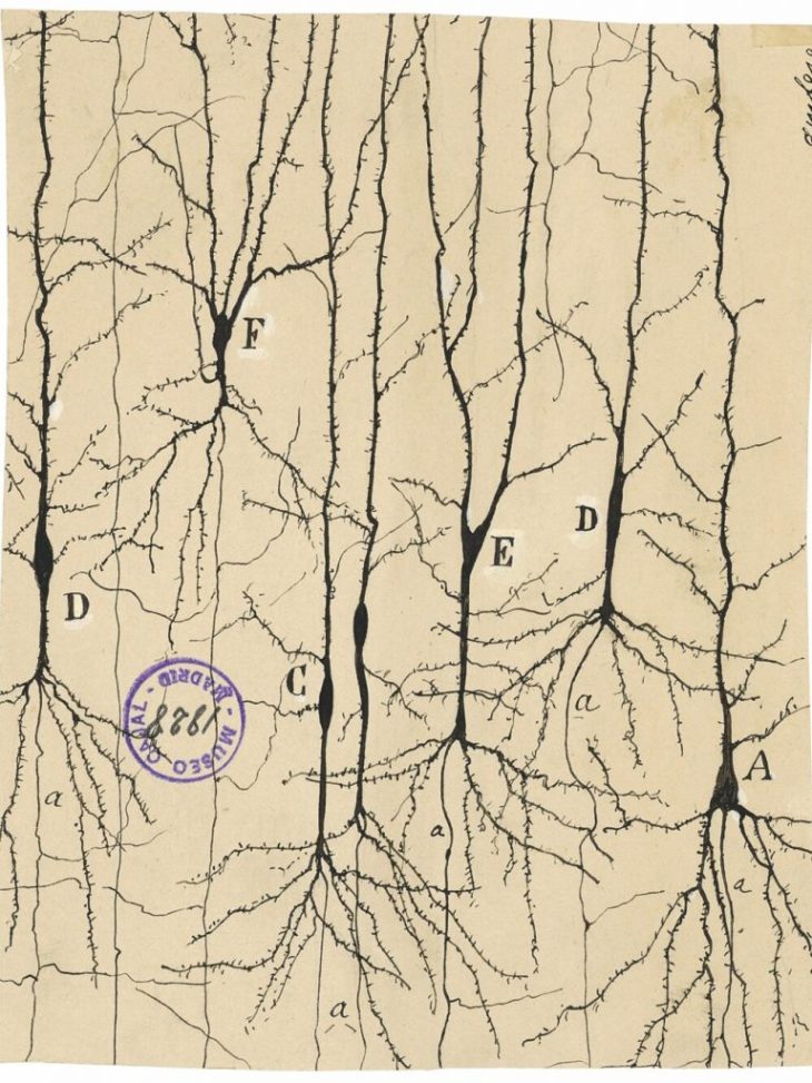
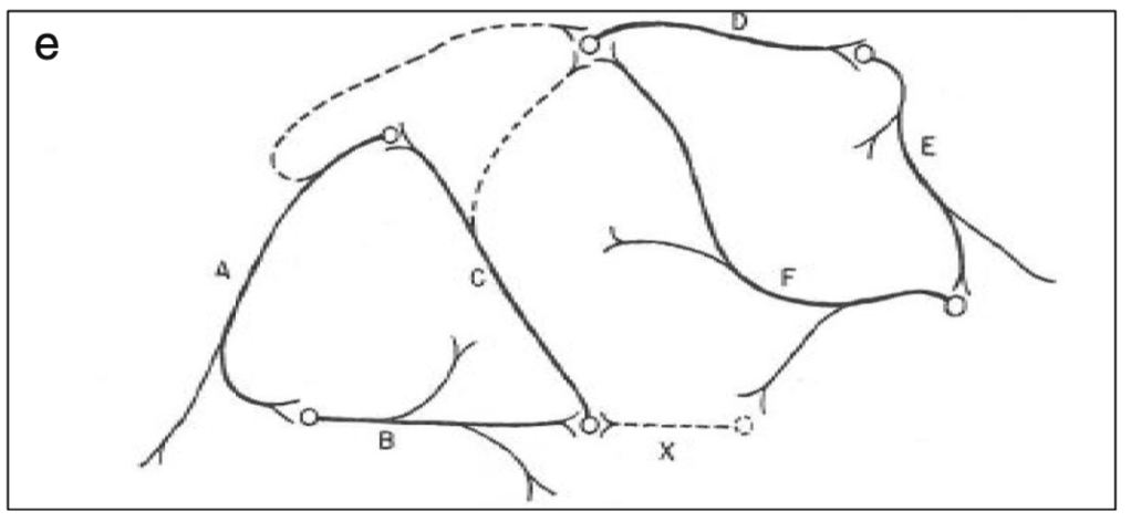
Ramon y Cajal (1888): Visualizing Neurons
The story begins with Santiago Ramon y Cajal (1853 – 1934) who received the Nobel Prize in physiology in 1906 for his work illuminating natural neural networks. He built on work by Camillo Golgi, using a stain to give intracellular components contrast [1], and then went further to developed his own silver emulsions like those of early photography (which was one of his hobbies). Cajal was the first to show that neurons were individual constituents of neural matter and that their contacts were sequential: axons of sets of neurons contacted the dendrites of other sets of neurons, never axon-to-axon or dendrite-to-dendrite, to create a complex communication network. This became known as the neuron doctrine, and it is a central idea of neuroscience today.
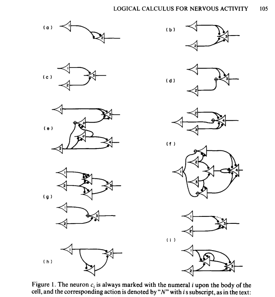
McCulloch and Pitts (1943): Mathematical Models
In 1941, Warren S. McCulloch (1898–1969) arrived at the Department of Psychiatry at the University of Illinois at Chicago where he met with the mathematical biology group at the University of Chicago led by Nicolas Rashevsky (1899–1972), widely acknowledged as the father of mathematical biophysics in the United States.
An itinerant member of Rashevsky’s group at the time was a brilliant, young and unusual mathematician, Walter Pitts (1923– 1969). He was not enrolled as a student at Chicago, but had simply “showed up” one day as a teenager at Rashevsky’s office door. Rashevsky was so impressed by Pitts that he invited him to attend the group meetings, and Pitts became interested in the application of mathematical logic to biological information systems.
When McCulloch met Pitts, he realized that Pitts had the mathematical background that complemented his own views of brain activity as computational processes. Pitts was homeless at the time, so McCulloch invited him to live with his family, giving the two men ample time to work together on their mutual obsession to provide a logical basis for brain activity in the way that Turing had provided it for computation.
McColloch and Pitts simplified the operation of individual neurons to their most fundamental character, envisioning a neural computing unit with multiple inputs (received from upstream neurons) and a single on-off output (sent to downstream neurons) with the additional possibility of feedback loops as downstream neurons fed back onto upstream neurons. They also discretized the dynamics in time, using discrete logic and time-difference equations, succeeding in devising a logical structure with rules and equations for the general operation of nets of neurons. They published their results a 1943 in the paper titled “A logical calculus of the ideas immanent in nervous activity,” [2] introducing computational language and logic to neuroscience. Their simplified neural unit became the basis for discrete logic, picked up a few years later by von Neumann as an elemental example of a logic gate upon which von Neumann began constructing the theory and design of the modern electronic computer.
Donald Hebb (1949): Hebbian Learning
The basic model for learning and adjustment of synaptic weights among neurons was put forward in 1949 by the physiological psychologist Donald Hebb (1904-1985) of McGill University in Canada in a book titled The Organization of Behavior [3].
In Hebbian learning, an initially untrained network consists of many neurons with many synapses having random synaptic weights. During learning, a synapse between two neurons is strengthened when both the pre-synaptic and post-synaptic neurons are firing simultaneously. In this model, it is essential that each neuron makes many synaptic contacts with other neurons because it requires many input neurons acting in concert to trigger the output neuron. In this way, synapses are strengthened when there is collective action among the neurons. The synaptic strengths are therefore altered through a form of self-organization. A collective response of the network strengthens all those synapses that are responsible for the response, while the other synapses that do not contribute, weaken. Despite the simplicity of this model, it has been surprisingly robust, standing up as a general principle for the training of artificial neural networks.
Hodgkin and Huxley (1952): Neuron Transporter Models
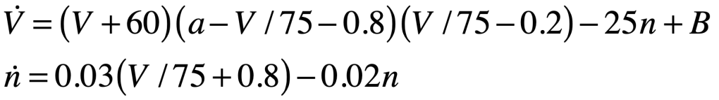
Alan Hodgkin (1914 – 1998) and Andrew Huxley (1917 – 2012) were English biophysicists who received the 1963 Nobel Prize in physiology for their work on the physics behind neural activation. They constructed a differential equation for the spiking action potential for which their biggest conceptual challenge was the presence of time delays in the voltage signals that were not explained by linear models of the neural conductance. As they began exploring nonlinear models, using their experiments to guide the choice of parameters, they settled on a dynamical model in a four-dimensional phase space. One dimension was voltage, while another was inhibitory current. The two remaining dimensions were sodium and potassium conductances, which they had determined were the major ions participating in the generation and propagation of the action potential. The nonlinear conductances of their model described the observed time delays and captured the essential neural behavior of the fast spike followed by a slow recovery. Huxley solved the equations on a hand-cranked calculator, taking over three months of tedious cranking to plot the numerical results.

Hodgkin and Huxley published [4] their measurements and their model (known as the Hodgkin-Huxley model) in a series of six papers in 1952 that led to an explosion of research in electrophysiology, for which Hodgkin and Huxley won the 1963 Nobel Prize in physiology or medicine. The four-dimensional Hodgkin–Huxley model stands as a classic example of the power of phenomenological modeling when combined with accurate experimental observation. Hodgkin and Huxley were able to ascertain not only the existence of ion channels in the cell membrane, but also their relative numbers, long before these molecular channels were ever directly observed using electron microscopes. The Hodgkin–Huxley model lent itself to simplifications that could capture the essential behavior of neurons while stripping off the details.
Frank Rosenblatt (1958): The Perceptron
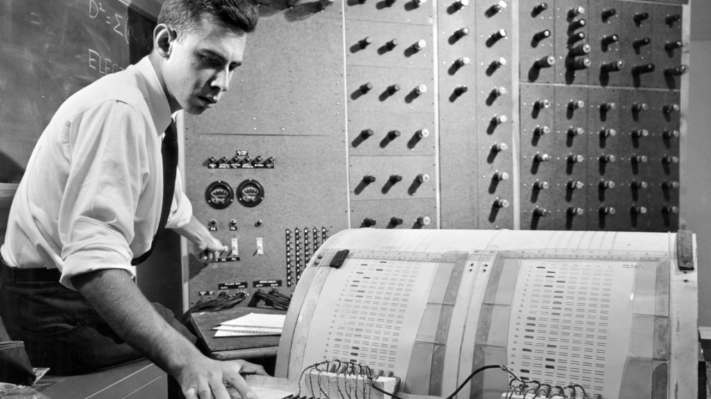
Frank Rosenblatt (1928–1971) had a PhD in psychology from Cornell University and was in charge of the cognitive systems section of the Cornell Aeronautical Laboratory (CAL) located in Buffalo, New York. He was tasked with fulfilling a contract from the Navy to develop an analog image processor. Drawing from the work of McCulloch and Pitts, his team constructed a software system and then constructed a hardware model that adaptively updated the strength of the inputs, that they called neural weights, as it was trained on test images. The machine was dubbed the Mark I Perceptron, and its announcement in 1958 created a small media frenzy [5]. A New York Times article reported the perceptron was “the embryo of an electronic computer that [the navy] expects will be able to walk, talk, see, write, reproduce itself and be conscious of its existence.”
The perceptron had a simple architecture, with two layers of neurons consisting of an input layer and a processing layer, and it was programmed by adjusting the synaptic weights to the inputs. This computing machine was the first to adaptively learn its functions, as opposed to following predetermined algorithms like digital computers. It seemed like a breakthrough in cognitive science and computing, as trumpeted by the New York Times. But within a decade, the development had stalled because the architecture was too restrictive.
Richard Fitzhugh and Jin-Ichi Nagumo (1961): Neural van der Pol Oscillators
In 1961 Richard FitzHugh (1922–2007), a neurophysiology researcher at the National Institute of Neurological Disease and Blindness (NINDB) of the National Institutes of Health (NIH), created a surprisingly simple model of the neuron that retained only a third order nonlinearity, just like the third-order nonlinearity that Rayleigh had proposed and solved in 1883, and that van der Pol extended in 1926. Around the same time that FitzHugh proposed his mathematical model [6], the electronics engineer Jin-Ichi Nagumo (1926-1999) in Japan created an electronic diode circuit with an equivalent circuit model that mimicked neural oscillations [7]. Together, this work by FitzHugh and Nagumo led to the so-called FitzHugh–Nagumo model. The conceptual importance of this model is that it demonstrated that the neuron was a self-oscillator, just like a violin string or wheel shimmy or the pacemaker cells of the heart. Once again, self-oscillators showed themselves to be common elements of a complex world—and especially of life.
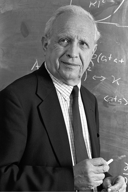
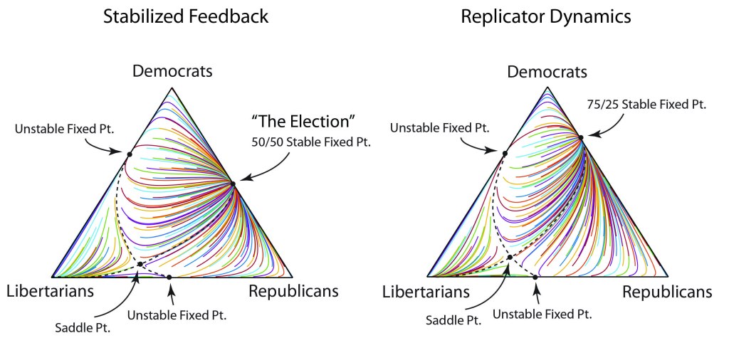
John Hopfield (1982): Spin Glasses and Recurrent Networks
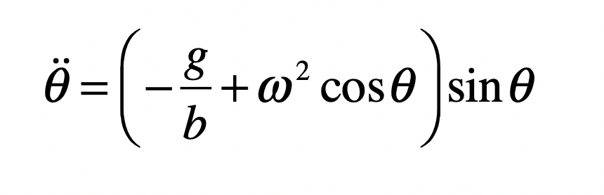
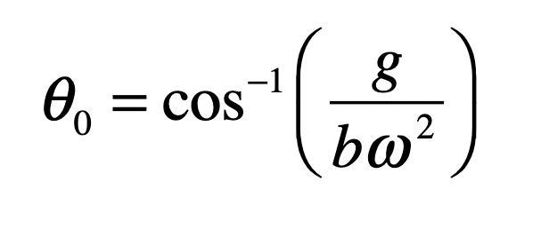
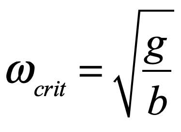
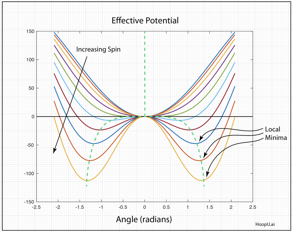
John Hopfield (1933–) received his PhD from Cornell University in 1958, advised by Al Overhauser in solid state theory, and he continued to work on a broad range of topics in solid state physics as he wandered from appointment to appointment at Bell Labs, Berkeley, Princeton, and Cal Tech. In the 1970s Hopfield’s interests broadened into the field of biophysics, where he used his expertise in quantum tunneling to study quantum effects in biomolecules, and expanded further to include information transfer processes in DNA and RNA. In the early 1980s, he became aware of aspects of neural network research and was struck by the similarities between McColloch and Pitts’ idealized neuronal units and the physics of magnetism. For instance, there is a type of disordered magnetic material called a spin glass in which a large number of local regions of magnetism are randomly oriented. In the language of solid-state physics, one says that the potential energy function of a spin glass has a large number of local minima into which various magnetic configurations can be trapped. In the language of dynamics, one says that the dynamical system has a large number of basins of attraction [8].
The Parallel Distributed Processing Group (1986): Backpropagation
David Rumelhart, a mathematical psychologist at UC San Diego, was joined by James McClelland in 1974 and then by Geoffrey Hinton in 1978 to become what they called the Parallel Distributed Processing (PDP) group. The central tenets of the PDP framework they developed were: 1) processing is distributed across many semi-autonomous neural units, that 2) learn by adjusting the weights of their interconnections based on the strengths of their signals (i.e., Hebbian learning), whose memories and behaviors are 3) an emergent property of the distributed learned weights.
PDP was an exciting framework for artificial intelligence, and it captured the general behavior of natural neural networks, but it had a serious problem: How could all of the neural weights be trained?
In 1986, Rumelhart and Hinton with the mathematician Ronald Williams developed a mathematical procedure for training neural weights called error backpropagation [9]. The idea is actually very simple: create a mean squared error of the response of a neural network compared to an ideal response, then tweak one of the neural weights and see if the error increases or decreases. If the error decreases, keep the tweak for that weight and move to the next, working iteratively, tweak by tweak, to minimize the mean squared error. In this way, large numbers of neural weights can be adjusted as the network is trained to perform a specified task.
Error backpropagation has come a long way from that early 1986 paper, and it now lies at the core of the AI revolution we are experiencing today as tens of millions of neural weights are trained on massive datasets.
Yann LeCun (1989): Convolutional Neural Networks
In 1988, I was a new post-doc at AT&T Bell Labs at Holmdel, New Jersey fresh out of my PhD in physics from Berkeley. Bell Labs liked to give its incoming employees inspirational talks and tours of their facilities, and one of the tours I took was of the neural network lab run by Lawrence Jackel that was working on computer recognition of zip-code digits. The team’s new post-doc, arriving at Bell Labs the same time as me, was Yann LeCun. It is very possible that the demo our little group watched was run by him, or at least he was there, but at the time he was a nobody, so even if I had heard his name, it wouldn’t have meant anything to me.
Fast forward to today, and Yann LeCun’s name is almost synonomous with AI. He is the Chief AI Scientist at Facebook and his google scholar page reports that he gets 50,000 citations per year.
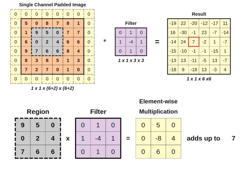
LeCun is famous for developing the convolutional neural network (CNN) in work that he published from Bell Labs in 1989 [10]. It is a biomimetic neural network that takes its inspiration from the receptive fields of the neural networks in the retina. What you think you see, when you look at something, is actually reconstructed by your brain. Your retina is a neural processor with receptive fields that are a far cry from one-to-one. Most prominent in the retina are center-surround fields, or kernels, that respond to the derivatives of the focused image instead of the image itself. It’s the derivatives that are sent up your optic neuron to your brain which then reconstructs the image. It works as a form of image compression so that broad uniform areas in an image are reduced to its edges.
The convolutional neural network works in the same way, it’s just engineered specifically to produce compressed and multiscale codes that capture broad areas as well as the fine details of an image. By constructing many different “kernel” operators at many different scales, it creates a set of features that capture the nuances of the image in quantitative form that is then processed by training neural weights in downstream neural networks.
Geoff Hinton (2006): Deep Belief
It seems like Geoff Hinton has had his finger in almost every pie when it comes to how we do AI today. Backpropagation? Geoff Hinton. Rectified Linear Units? Geoff Hinton. Boltzmann Machines? Geoff Hinton. t-SNE? Geoff Hinton. Dropout regularization? Geoff Hinton. AlexNet? Geoff Hinton. The 2024 Nobel Prize in Physics? Geoff Hinton! He may not have invented all of these, but he was in the midst of it all.
Hinton received his PhD in Artificial Intelligence (ar rare field at the time) from the University of Edinburgh in 1978 after which he joined the PDP group at UCSD (see above) as a post-doc. After a time at Carnegie-Mellon, he joined the University of Toronto, Canada, in 1987 where he established one of the leading groups in the world on neural network research. It was from here that he launched so many of the ideas and techniques that have become the core of deep learning.
A central idea of deep learning came from Hinton’s work on Boltzmann Machines that learn statistical distributions of complex data. This type of neural network is known as an energy-based model, similar to a Hopfield network, and it has strong ties to the statistical mechanics of spin-glass systems. Unfortunately, it is a bitch to train! So Hinton simplified it into a Restricted Boltzmann Machine (RBM) that was much more tractable and layers of RBMs could be stacked into “Deep Belief Networks” [11] that had a hierarchical structure that allowed the neural nets to learn layers of abstractions. These were among the first deep networks that were able to do complex tasks at the level of human capabilities (and sometimes beyond).
The breakthrough that propelled Geoff Hinton to world-wide acclaim was the success of AlexNet, a neural network constructed by his graduate student Alex Krizhevsky at Toronto in 2012 consisting of 650,000 neurons with 60 million parameters that were trained using two early Nvidia GPUs. It won the ImageNet challenge that year, enabled by its deep architecture and representing a marked advancement that has been proceeding unabated today.
Deep learning is now the rule in AI, supported by the Attention mechanism and Transformers that underpin the large language models, like ChatGPT and others, that are poised to disrupt all the legacy business models based on the previous silicon revolution of 50 years ago.
Further Reading

References
[1] Ramón y Cajal S. (1888). Estructura de los centros nerviosos de las aves. Rev. Trim. Histol. Norm. Pat. 1, 1–10.
[2] McCulloch, W.S. and W. Pitts, A Logical Calculus of the Ideas Immanent in Nervous Activity. Bull. Math. Biophys., 1943. 5: p. 115.
[3] Hebb, D. O. (1949). The Organization of Behavior: A Neuropsychological Theory. New York: Wiley and Sons. ISBN 978-0-471-36727-7 – via Internet Archive.
[4] Hodgkin AL, Huxley AF (August 1952). “A quantitative description of membrane current and its application to conduction and excitation in nerve”. The Journal of Physiology. 117 (4): 500–44.
[5] Rosenblatt, Frank (1957). “The Perceptron—a perceiving and recognizing automaton”. Report 85-460-1. Cornell Aeronautical Laboratory.
[6] FitzHugh, Richard (July 1961). “Impulses and Physiological States in Theoretical Models of Nerve Membrane”. Biophysical Journal. 1 (6): 445–466.
[7] Nagumo, J.; Arimoto, S.; Yoshizawa, S. (October 1962). “An Active Pulse Transmission Line Simulating Nerve Axon”. Proceedings of the IRE. 50 (10): 2061–2070.
[8] Hopfield, J. J. (1982). “Neural networks and physical systems with emergent collective computational abilities”. Proceedings of the National Academy of Sciences. 79 (8): 2554–2558.
[9] Rumelhart, D.E. et al. Nature 323, 533-536 (1986).
[10] Y. LeCun, B. Boser, J. S. Denker, D. Henderson, R. E. Howard, W. Hubbard and L. D. Jackel: Backpropagation Applied to Handwritten Zip Code Recognition, Neural Computation, 1(4):541–551, Winter 1989.
[11] G. E. Hinton, S. Osindero, and Y. W. Teh, “A fast learning algorithm for deep belief nets,” Neural Computation 18, 1527-1554 (2006).