This is the fourth installment in a series of blogs on the population dynamics of COVID-19. In my first blog I looked at a bifurcation physics model that held the possibility (and hope) that with sufficient preventive action the pandemic could have died out and spared millions. That hope was in vain.
What will it be like to live with COVID-19 as a constant factor of modern life for years to come?
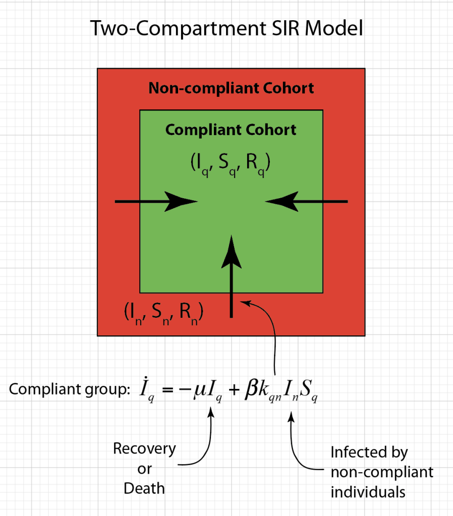
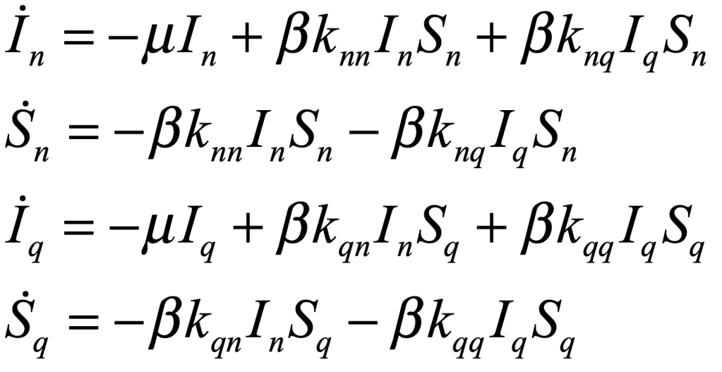
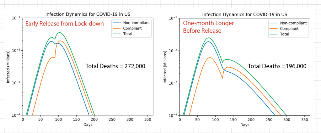
In my second blog I looked at a two-component population dynamics model that showed the importance of locking down and not emerging too soon. It predicted that waiting only a few extra weeks before opening could have saved tens of thousands of lives. Unfortunately, because states like Texas and Florida opened too soon and refused to mandate the wearing of masks, thousands of lives were lost.
In my third blog I looked at a network physics model that showed the importance of rapid testing and contact tracing to remove infected individuals to push the infection rate low — not only to flatten the curve, but to drive it down. While most of the developed world is succeeding in achieving this, the United States is not.
In this fourth blog, I am looking at a simple mean-field model that shows what it will be like to live with COVID-19 as a constant factor of modern life for years to come. This is what will happen if the period of immunity to the disease is short and people who recover from the disease can get it again. Then the disease will never go away and the world will need to learn to deal with it. How different that world will look from the one we had just a year ago will depend on the degree of immunity that is acquired after infection, how long a vaccine will provide protection before booster shots are needed, and how many people will get the vaccine or will refus.
SIRS for SARS
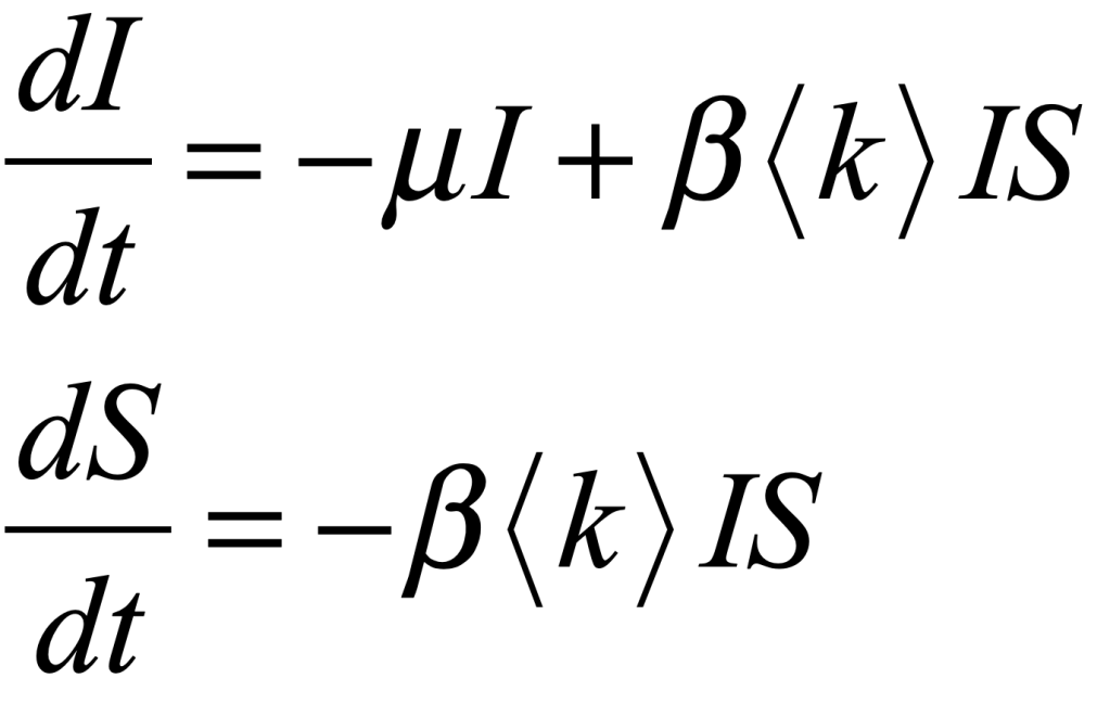
COVID-19 is a SARS corona virus known as SARS-CoV-2. SARS stands for Severe Acute Respiratory Syndrome. There is a simple and well-established mean-field model for an infectious disease like SARS that infects individuals, from which they recover, but after some lag period they become susceptible again. This is called the SIRS model, standing for Susceptible-Infected-Recovered-Susceptible. This model is similar to the SIS model of my first blog, but it now includes a mean lifetime for the acquired immunity, after an individual recovers from the infection and then becomes susceptible again. The bifurcation threshold is the same for the SIRS model as the SIS model, but with SIRS there is a constant susceptible population. The mathematical flow equations for this model are

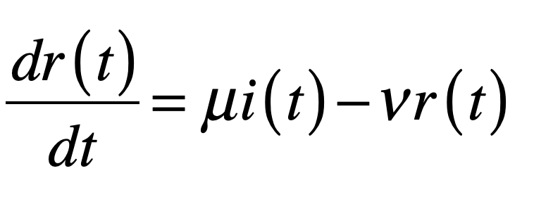
where i is the infected fraction, r is the recovered fraction, and 1 – i – r = s is the susceptible fraction. The infection rate for an individual who has k contacts is βk. The recovery rate is μ and the mean lifetime of acquired immunity after recovery is τlife = 1/ν. This model assumes that all individuals are equivalent (no predispositions) and there is no vaccine–only natural immunity that fades in time after recovery.
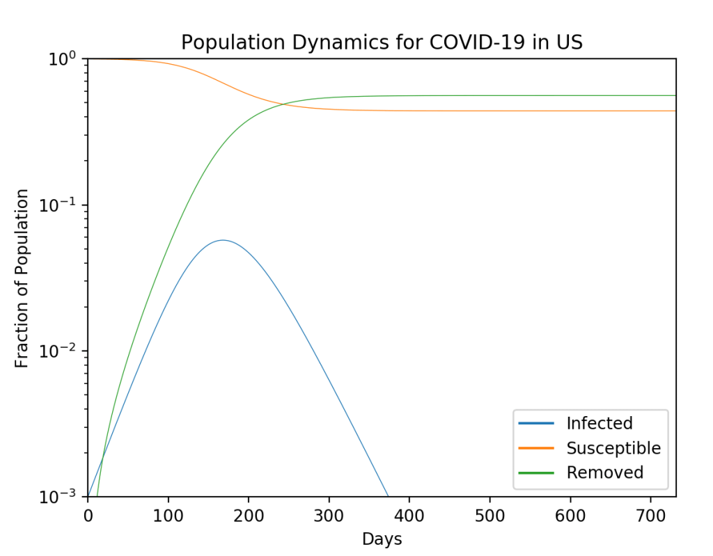
The population trajectories for this model are shown in Fig. 1. The figure on the left is a 3-simplex where every point in the triangle stands for a 3-tuple (i, r, s). Our own trajectory starts at the right bottom vertex and generates the green trajectory that spirals into the fixed point. The parameters are chosen to be roughly equivalent to what is known about the virus (but with big uncertainties in the model parameters). One of the key results is that the infection will oscillate over several years, settling into a steady state after about 4 years. Thereafter, there is a steady 3% infected population with 67% of the population susceptible and 30% recovered. The decay time for the immunity is assumed to be one year in this model. Note that the first peak in the infected numbers will be about 1 year, or around March 2021. There is a second smaller peak (the graph on the right is on a vertical log scale) at about 4 years, or sometime in 2024.

Although the recovered fraction is around 30% for these parameters, it is important to understand that this is a dynamic equilibrium. If there is no vaccine, then any individual who was once infected can be infected again after about a year. So if they don’t get the disease in the first year, they still have about a 4% chance to get it every following year. In 50 years, a 20-year-old today would have almost a 90% chance of having been infected at least once and an 80% chance of having gotten it at least twice. In other words, if there is never a vaccine, and if immunity fades after each recovery, then almost everyone will eventually get the disease several times in their lifetime. Furthermore, COVID will become the third most likely cause of death in the US after heart disease (first) and cancer (second). The sad part of this story is that it all could have been avoided if the government leaders of several key nations, along with their populations, had behaved responsibly.
The Asymmetry of Personal Cost under COVID
The nightly news in the US during the summer of 2020 shows endless videos of large parties, dense with people, mostly young, wearing no masks. This is actually understandable even though regrettable. It is because of the asymmetry of personal cost. Here is what that means …
On any given day, an individual who goes out and about in the US has only about a 0.01 percent chance of contracting the virus. In the entire year, there is only about a 3% chance that that individual will get the disease. And even if they get the virus, they only have a 2% chance of dying. So the actual danger per day per person is so minuscule that it is hard to understand why it is so necessary to wear a mask and socially distance. Therefore, if you go out and don’t wear a mask, almost nothing bad will happen to YOU. So why not? Why not screw the masks and just go out!
And this is why that’s such a bad idea: because if no-one wears a mask, then tens or hundreds of thousands of OTHERS will die.
This is the asymmetry of personal cost. By ignoring distancing, nothing is likely to happen to YOU, but thousands of OTHERS will die. How much of your own comfort are you willing to give up to save others? That is the existential question.
This year is the 75th anniversary of the end of WW II. During the war everyone rationed and recycled, not because they needed it for themselves, but because it was needed for the war effort. Almost no one hesitated back then. It was the right thing to do even though it cost personal comfort. There was a sense of community spirit and doing what was good for the country. Where is that spirit today? The COVID-19 pandemic is a war just as deadly as any war since WW II. There is a community need to battle it. All anyone has to do is wear a mask and behave responsibly. Is this such a high personal cost?
The Vaccine
All of this can change if a reliable vaccine can be developed. There is no guarantee that this can be done. For instance, there has never been a reliable vaccine for the common cold. A more sobering thought is to realize is that there has never been a vaccine for the closely related virus SARS-CoV-1 that broke out in 2003 in China but was less infectious. But the need is greater now, so there is reason for optimism that a vaccine can be developed that elicits the production of antibodies with a mean lifetime at least as long as for naturally-acquired immunity.
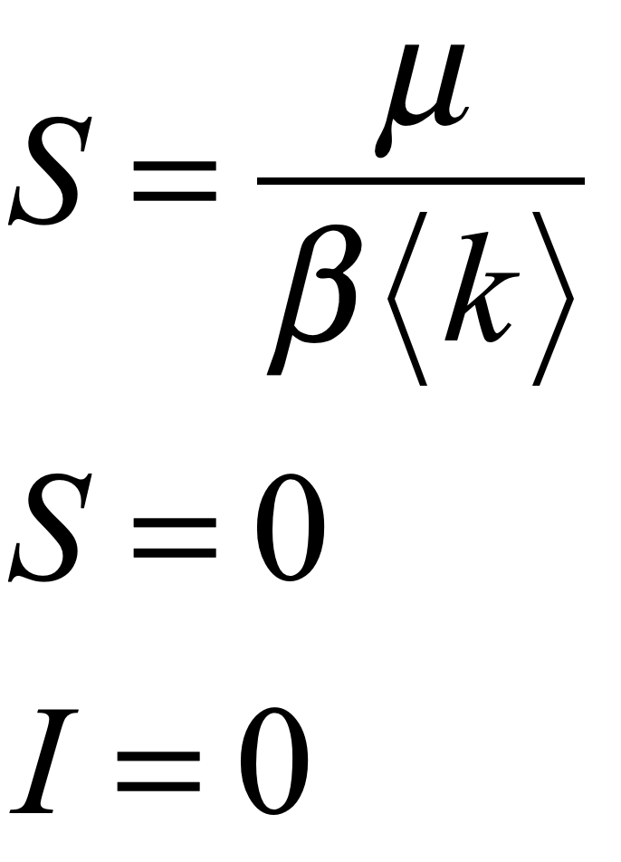
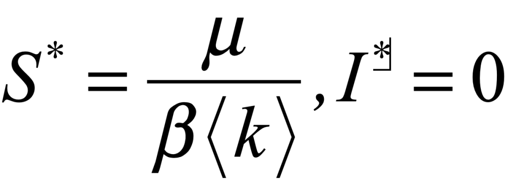
The SIRS model has the same bifurcation threshold as the SIS model that was discussed in a previous blog. If the infection rate can be made slower than the recovery rate, then the pandemic can be eliminated entirely. The threshold is
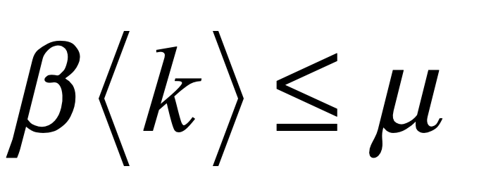
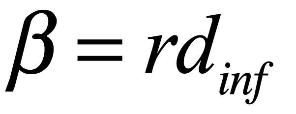
The parameter μ, the recovery rate, is intrinsic and cannot be changed. The parameter β, the infection rate per contact, can be reduced by personal hygiene and wearing masks. The parameter <k>, the average number of contacts to a susceptible person, can be significantly reduced by vaccinating a large fraction of the population.
To simulate the effect of vaccination, the average <k> per person can be reduced at the time of vaccination. This lowers the average infection rate. The results are shown in Fig. 2 for the original dynamics, a vaccination of 20% of the populace, and a vaccination of 40% of the populace. For 20% vaccination, the epidemic is still above threshold, although the long-time infection is lower. For 40% of the population vaccinated, the disease falls below threshold and would decay away and vanish.
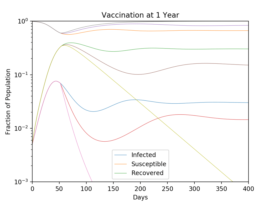
In this model, the vaccination is assumed to decay at the same rate as naturally acquired immunity (one year), so booster shots would be needed every year. Getting 40% of the population to get vaccinated may be achieved. Roughly that fraction get yearly flu shots in the US, so the COVID vaccine could be added to the list. But at 40% it would still be necessary for everyone to wear face masks and socially distance until the pandemic fades away. Interestingly, if the 40% got vaccinated all on the same date (across the world), then the pandemic would be gone in a few months. Unfortunately, that’s unrealistic, so with a world-wide push to get 40% of the World’s population vaccinated within five years, it would take that long to eliminate the disease, taking us to 2025 before we could go back to the way things were in November of 2019. But that would take a world-wide vaccination blitz the likes of which the world has never seen.
Python Code: SIRS.py
#!/usr/bin/env python3
# -*- coding: utf-8 -*-
"""
SIRS.py
Created on Fri July 17 2020
D. D. Nolte, "Introduction to Modern Dynamics:
    Chaos, Networks, Space and Time, 2nd Edition (Oxford University Press, 2019)
@author: nolte
"""

import numpy as np
from scipy import integrate
from matplotlib import pyplot as plt

plt.close('all')

def tripartite(x,y,z):

    sm = x + y + z
    xp = x/sm
    yp = y/sm

    f = np.sqrt(3)/2

    y0 = f*xp
    x0 = -0.5*xp - yp + 1;

    lines = plt.plot(x0,y0)
    plt.setp(lines, linewidth=0.5)
    plt.plot([0, 1],[0, 0],'k',linewidth=1)
    plt.plot([0, 0.5],[0, f],'k',linewidth=1)
    plt.plot([1, 0.5],[0, f],'k',linewidth=1)
    plt.show()

print(' ')
print('SIRS.py')

def solve_flow(param,max_time=1000.0):

    def flow_deriv(x_y,tspan,mu,betap,nu):
        x, y = x_y

        return [-mu*x + betap*x*(1-x-y),mu*x-nu*y]

    x0 = [del1, del2]

    # Solve for the trajectories
    t = np.linspace(0, int(tlim), int(250*tlim))
    x_t = integrate.odeint(flow_deriv, x0, t, param)

    return t, x_t

 # rates per week
betap = 0.3;   # infection rate
mu = 0.2;      # recovery rate
nu = 0.02      # immunity decay rate

print('beta = ',betap)
print('mu = ',mu)
print('nu =',nu)
print('betap/mu = ',betap/mu)

del1 = 0.005         # initial infected
del2 = 0.005         # recovered

tlim = 600          # weeks (about 12 years)

param = (mu, betap, nu)    # flow parameters

t, y = solve_flow(param)
I = y[:,0]
R = y[:,1]
S = 1 - I - R

plt.figure(1)
lines = plt.semilogy(t,I,t,S,t,R)
plt.ylim([0.001,1])
plt.xlim([0,tlim])
plt.legend(('Infected','Susceptible','Recovered'))
plt.setp(lines, linewidth=0.5)
plt.xlabel('Days')
plt.ylabel('Fraction of Population')
plt.title('Population Dynamics for COVID-19')
plt.show()

plt.figure(2)
plt.hold(True)
for xloop in range(0,10):
    del1 = xloop/10.1 + 0.001
    del2 = 0.01

    tlim = 300
    param = (mu, betap, nu)    # flow parameters
    t, y = solve_flow(param)
    I = y[:,0]
    R = y[:,1]
    S = 1 - I - R

    tripartite(I,R,S);

for yloop in range(1,6):
    del1 = 0.001;
    del2 = yloop/10.1
    t, y = solve_flow(param)
    I = y[:,0]
    R = y[:,1]
    S = 1 - I - R

    tripartite(I,R,S);

for loop in range(2,10):
    del1 = loop/10.1
    del2 = 1 - del1 - 0.01
    t, y = solve_flow(param)
    I = y[:,0]
    R = y[:,1]
    S = 1 - I - R

    tripartite(I,R,S);

plt.hold(False)
plt.title('Simplex Plot of COVID-19 Pop Dynamics')

vac = [1, 0.8, 0.6]
for loop in vac:

    # Run the epidemic to the first peak
    del1 = 0.005
    del2 = 0.005
    tlim = 52
    param = (mu, betap, nu)
    t1, y1 = solve_flow(param)

    # Now vaccinate a fraction of the population
    st = np.size(t1)
    del1 = y1[st-1,0]
    del2 = y1[st-1,1]
    tlim = 400

    param = (mu, loop*betap, nu)
    t2, y2 = solve_flow(param)

    t2 = t2 + t1[st-1]

    tc = np.concatenate((t1,t2))
    yc = np.concatenate((y1,y2))

    I = yc[:,0]
    R = yc[:,1]
    S = 1 - I - R

    plt.figure(3)
    plt.hold(True)
    lines = plt.semilogy(tc,I,tc,S,tc,R)
    plt.ylim([0.001,1])
    plt.xlim([0,tlim])
    plt.legend(('Infected','Susceptible','Recovered'))
    plt.setp(lines, linewidth=0.5)
    plt.xlabel('Weeks')
    plt.ylabel('Fraction of Population')
    plt.title('Vaccination at 1 Year')
    plt.show()

plt.hold(False)
Caveats and Disclaimers
No effort was made to match parameters to the actual properties of the COVID-19 pandemic. The SIRS model is extremely simplistic and can only show general trends because it homogenizes away all the important spatial heterogeneity of the disease across the cities and states of the country. If you live in a hot spot, this model says little about what you will experience locally. The decay of immunity is also a completely open question and the decay rate is completely unknown. It is easy to modify the Python program to explore the effects of differing decay rates and vaccination fractions. The model also can be viewed as a “compartment” to model local variations in parameters.
