Since my last Blog on the bifurcation physics of COVID-19, most of the US has approached the crest of “the wave”, with the crest arriving sooner in hot spots like New York City and a few weeks later in rural areas like Lafayette, Indiana where I live. As of the posting of this Blog, most of the US is in lock-down with only a few hold-out states. Fortunately, this was sufficient to avoid the worst case scenarios of my last Blog, but we are still facing severe challenges.

There is good news! The second wave can be managed and minimized if we don’t come out of lock-down too soon.

One fall-out of the (absolutely necessary) lock-down is the serious damage done to the economy that is now in its greatest retraction since the Great Depression. The longer the lock-down goes, the deeper the damage and the longer to recover. The single-most important question at this point in time, as we approach the crest, is when we can emerge from lock down? This is a critical question. If we emerge too early, then the pandemic will re-kindle into a second wave that could exceed the first. But if we emerge later than necessary, then the economy may take a decade to fully recover. We need a Goldilocks solution: not too early and not too late. How do we assess that?

The Value of Qualitative Physics

In my previous Blog I laid out a very simple model called the Susceptible-Infected-Removed (SIR) model and provided a Python program whose parameters can be tweaked to explore the qualitatitive behavior of the model, answering questions like: What is the effect of longer or shorter quarantine periods? What role does social distancing play in saving lives? What happens if only a small fraction of the population pays attention and practice social distancing?

It is necessary to wait from releasing the lock-down at least several weeks after the crest has passed to avoid the second wave.

It is important to note that none of the parameters in that SIR model are reliable and no attempt was made to fit the parameters to the actual data. To expert epidemiological modelers, this simplistic model is less than useless and potentially dangerous if wrong conclusions are arrived at and disseminated on the internet.

But here is the point: The actual numbers are less important than the functional dependences. What matters is how the solution changes as a parameter is changed. The Python programs allow non-experts to gain an intuitive understanding of the qualitative physics of the pandemic. For instance, it is valuable to gain a feeling of how sensitive the pandemic is to small changes in parameters. This is especially important because of the bifurcation physics of COVID-19 where very small changes can cause very different trajectories of the population dynamics.

In the spirit of the value of qualitative physics, I am extending here that simple SIR model to a slightly more sophisticated model that can help us understand the issues and parametric dependences of this question of when to emerge from lock-down. Again, no effort is made to fit actual data of this pandemic, but there are still important qualitative conclusions to be made.

The Two-Compartment SIR Model of COVID-19

To approach a qualitative understanding of what happens by varying the length of time of the country-wide shelter-in-place, it helps to think of two cohorts of the public: those who are compliant and conscientious valuing the lives of others, and those who don’t care and are non-compliant.

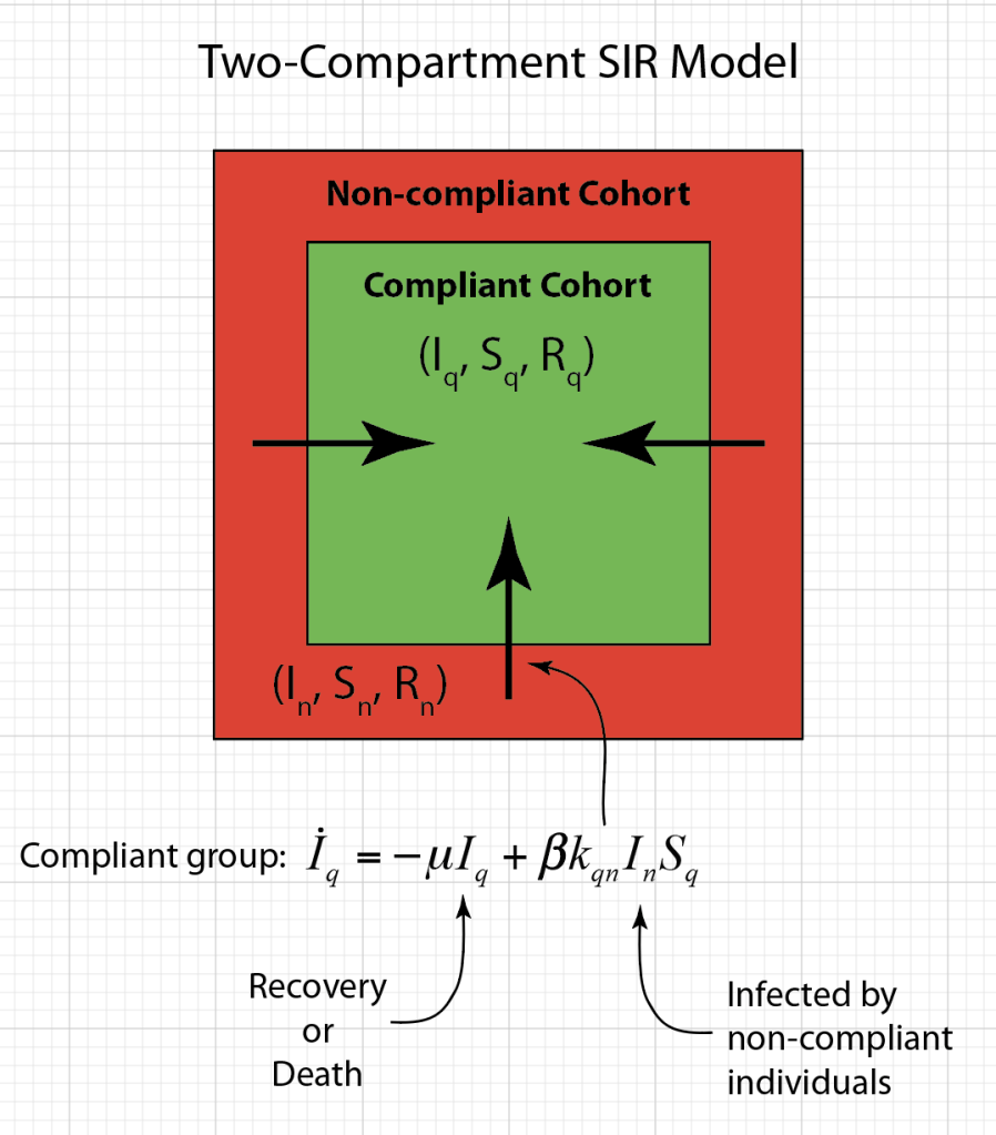
These two cohorts can each be modeled separately by their own homogeneous SIR models, but with a coupling between them because even those who shelter in place must go out for food and medicines. The equations of this two-compartment model are

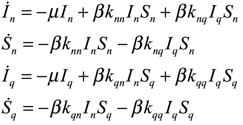
where n and q refer to the non-compliant and the compliant cohorts, respectively. I and S are the susceptible populations. The coupling parameters are knn for the coupling between non-compliants individuals, knq for the effect of the compliant individuals on the non-compliant, kqn for the effect of the non-compliant individuals on the compliant, and kqq for the effect of the compliant cohort on themselves.

There are two time frames for the model. The first time frame is the time of lock-down when the compliant cohort is sheltering in place and practicing good hygiene, but they still need to go out for food and medicines. (This model does not include the first responders. They are an important cohort, but do not make up a large fraction of the national population). The second time frame is after the lock-down is removed. Even then, good practices by the compliant group are expected to continue with the purpose to lower infections among themselves and among others.

This two-compartment model has roughly 8 adjustable parameters, all of which can be varied to study their effects on the predictions. None of them are well known, but general trends still can be explored.

Python Code: SIRWave.py

#!/usr/bin/env python3
# -*- coding: utf-8 -*-
"""
SIRWave.py
Created on Sat March 21 2020
@author: nolte
D. D. Nolte, Introduction to Modern Dynamics: Chaos, Networks, Space and Time, 2nd ed. (Oxford,2019)
"""

import numpy as np
from scipy import integrate
from matplotlib import pyplot as plt

plt.close('all')

print(' ')
print('SIRWave.py')

def solve_flow(param,max_time=1000.0):

    def flow_deriv(x_y_z_w,tspan):
        In, Sn, Iq, Sq = x_y_z_w
        
        Inp = -mu*In + beta*knn*In*Sn + beta*knq*Iq*Sn
        Snp = -beta*knn*In*Sn - beta*knq*Iq*Sn
        
        Iqp = -mu*Iq + beta*kqn*In*Sq + beta*kqq*Iq*Sq
        Sqp = -beta*kqn*In*Sq - beta*kqq*Iq*Sq
        
        return [Inp, Snp, Iqp, Sqp]
    
    x0 = [In0, Sn0, Iq0, Sq0]
    
    # Solve for the trajectories
    t = np.linspace(tlo, thi, thi-tlo)
    x_t = integrate.odeint(flow_deriv, x0, t)

    return t, x_t

beta = 0.02   # infection rate
dill = 5      # mean days infectious
mu = 1/dill   # decay rate
fnq = 0.3     # fraction not quarantining
fq = 1-fnq    # fraction quarantining
P = 330       # Population of the US in millions
mr = 0.002    # Mortality rate
dq = 90       # Days of lock-down (this is the key parameter)

# During quarantine
knn = 50      # Average connections per day for non-compliant group among themselves
kqq = 0       # Connections among compliant group
knq = 0       # Effect of compliaht group on non-compliant
kqn = 5       # Effect of non-clmpliant group on compliant

initfrac = 0.0001          # Initial conditions:
In0 = initfrac*fnq         # infected non-compliant
Sn0 = (1-initfrac)*fnq     # susceptible non-compliant
Iq0 = initfrac*fq          # infected compliant
Sq0 = (1-initfrac)*fq      # susceptivle compliant

tlo = 0
thi = dq

param = (mu, beta, knn, knq, kqn, kqq)    # flow parameters

t1, y1 = solve_flow(param)

In1 = y1[:,0]
Sn1 = y1[:,1]
Rn1 = fnq - In1 - Sn1
Iq1 = y1[:,2]
Sq1 = y1[:,3]
Rq1 = fq - Iq1 - Sq1

# Lift the quarantine: Compliant group continues social distancing
knn = 50      # Adjusted coupling parameters
kqq = 5
knq = 20
kqn = 15

fin1 = len(t1)
In0 = In1[fin1-1]
Sn0 = Sn1[fin1-1]
Iq0 = Iq1[fin1-1]
Sq0 = Sq1[fin1-1]

tlo = fin1
thi = fin1 + 365-dq

param = (mu, beta, knn, knq, kqn, kqq)

t2, y2 = solve_flow(param)

In2 = y2[:,0]
Sn2 = y2[:,1]
Rn2 = fnq - In2 - Sn2
Iq2 = y2[:,2]
Sq2 = y2[:,3]
Rq2 = fq - Iq2 - Sq2

fin2 = len(t2)
t = np.zeros(shape=(fin1+fin2,))
In = np.zeros(shape=(fin1+fin2,))
Sn = np.zeros(shape=(fin1+fin2,))
Rn = np.zeros(shape=(fin1+fin2,))
Iq = np.zeros(shape=(fin1+fin2,))
Sq = np.zeros(shape=(fin1+fin2,))
Rq = np.zeros(shape=(fin1+fin2,))

t[0:fin1] = t1
In[0:fin1] = In1
Sn[0:fin1] = Sn1
Rn[0:fin1] = Rn1
Iq[0:fin1] = Iq1
Sq[0:fin1] = Sq1
Rq[0:fin1] = Rq1

t[fin1:fin1+fin2] = t2
In[fin1:fin1+fin2] = In2
Sn[fin1:fin1+fin2] = Sn2
Rn[fin1:fin1+fin2] = Rn2
Iq[fin1:fin1+fin2] = Iq2
Sq[fin1:fin1+fin2] = Sq2
Rq[fin1:fin1+fin2] = Rq2

plt.figure(1)
lines = plt.semilogy(t,In,t,Iq,t,(In+Iq))
plt.ylim([0.0001,.1])
plt.xlim([0,thi])
plt.legend(('Non-compliant','Compliant','Total'))
plt.setp(lines, linewidth=0.5)
plt.xlabel('Days')
plt.ylabel('Infected')
plt.title('Infection Dynamics for COVID-19 in US')
plt.show()

plt.figure(2)
lines = plt.semilogy(t,Rn*P*mr,t,Rq*P*mr)
plt.ylim([0.001,1])
plt.xlim([0,thi])
plt.legend(('Non-compliant','Compliant'))
plt.setp(lines, linewidth=0.5)
plt.xlabel('Days')
plt.ylabel('Deaths')
plt.title('Total Deaths for COVID-19 in US')
plt.show()

D = P*mr*(Rn[fin1+fin2-1] + Rq[fin1+fin2-1])
print('Deaths = ',D)

plt.figure(3)
lines = plt.semilogy(t,In/fnq,t,Iq/fq)
plt.ylim([0.0001,.1])
plt.xlim([0,thi])
plt.legend(('Non-compliant','Compliant'))
plt.setp(lines, linewidth=0.5)
plt.xlabel('Days')
plt.ylabel('Fraction of Sub-Population')
plt.title('Population Dynamics for COVID-19 in US')
plt.show()

Trends

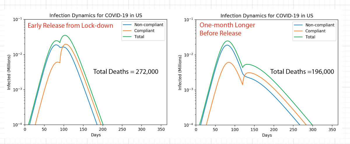
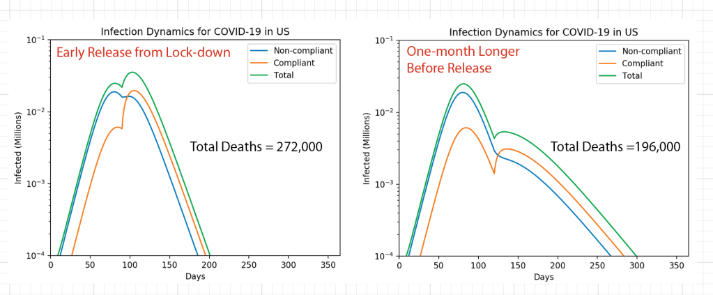
The obvious trend to explore is the effect of changing the quarantine period. Fig. 2 shows the results of a an early release from shelter-in-place compared to pushing the release date one month longer. The trends are:

• If the lock-down is released early, the second wave can be larger than the first wave
• If the lock-down is released early, the compliant cohort will be mostly susceptible and will have the majority of new cases
• There are 40% more deaths when the lock-down is released early

If the lock-down is ended just after the crest, this is too early. It is necessary to wait at least several weeks after the crest has passed to avoid the second wave. There are almost 40% more deaths for the 90-day period than the 120-day period. In addition, for the case when the quarantine is stopped too early, the compliant cohort, since they are the larger fraction and are mostly susceptible, will suffer a worse number of new infections than the non-compliant group who put them at risk in the first place. In addition, the second wave for the compliant group would be worse than the first wave. This would be a travesty! But by pushing the quarantine out by just 1 additional month, the compliant group will suffer fewer total deaths than the non-compliant group. Most importantly, the second wave would be substantially smaller than the first wave for both cohorts.

The lesson from this simple model is simple: push the quarantine date out as far as the economy can allow! There is good news! The second wave can be managed and minimized if we don’t come out of lock-down too soon.

Caveats and Disclaimers

This model is purely qualitative and only has value for studying trends that depend on changing parameters. Absolute numbers are not meant to be taken too seriously. For instance, the total number of deaths in this model are about 2x larger than what we are hearing from Dr. Fauci of NIAID at this time, so this simple model overestimates fatalities. Also, it doesn’t matter whether the number of quarantine days should be 60, 90 or 120 … what matters is that an additional month makes a large difference in total number of deaths. If someone does want to model the best possible number of quarantine days — the Goldilocks solution — then they need to get their hands on a professional epidemiological model (or an actual epidemiologist). The model presented here is not appropriate for that purpose.

Note added in postscript on April 8: Since posting the original blog on April 6, Dr, Fauci announced that as many as 90% of individuals are practicing some form of social distancing. In addition, many infections are not being reported because of lack of testing, which means that the mortality rate is lower than thought. Therefore, I have changed the mortality rate and figures with numbers that better reflect the current situation (that is changing daily), but still without any attempt to fit the numerous other parameters.