

If you are a fan of the Doppler effect, then time trials at the Indy 500 Speedway will floor you. Even if you have experienced the fall in pitch of a passing train whistle while stopped in your car at a railroad crossing, or heard the falling whine of a jet passing overhead, I can guarantee that you have never heard anything like an Indy car passing you by at 225 miles an hour.
Indy 500 Time Trials and the Doppler Effect
The Indy 500 time trials are the best way to experience the effect, rather than on race day when there is so much crowd noise and the overlapping sounds of all the cars. During the week before the race, the cars go out on the track, one by one, in time trials to decide the starting order in the pack on race day. Fans are allowed to wander around the entire complex, so you can get right up to the fence at track level on the straight-away. The cars go by only thirty feet away, so they are coming almost straight at you as they approach and straight away from you as they leave. The whine of the car as it approaches is 43% higher than when it is standing still, and it drops to 33% lower than the standing frequency—a ratio almost approaching a factor of two. And they go past so fast, it is almost a step function, going from a steady high note to a steady low note in less than a second. That is the Doppler effect!
But as obvious as the acoustic Doppler effect is to us today, it was far from obvious when it was proposed in 1842 by Christian Doppler at a time when trains, the fastest mode of transport at the time, ran at 20 miles per hour or less. In fact, Doppler’s theory generated so much controversy that the Academy of Sciences of Vienna held a trial in 1853 to decide its merit—and Doppler lost! For the surprising story of Doppler and the fate of his discovery, see my Physics Today article.
From that fraught beginning, the effect has expanded in such importance, that today it is a daily part of our lives. From Doppler weather radar, to speed traps on the highway, to ultrasound images of babies—Doppler is everywhere.
Development of the Doppler-Fizeau Effect
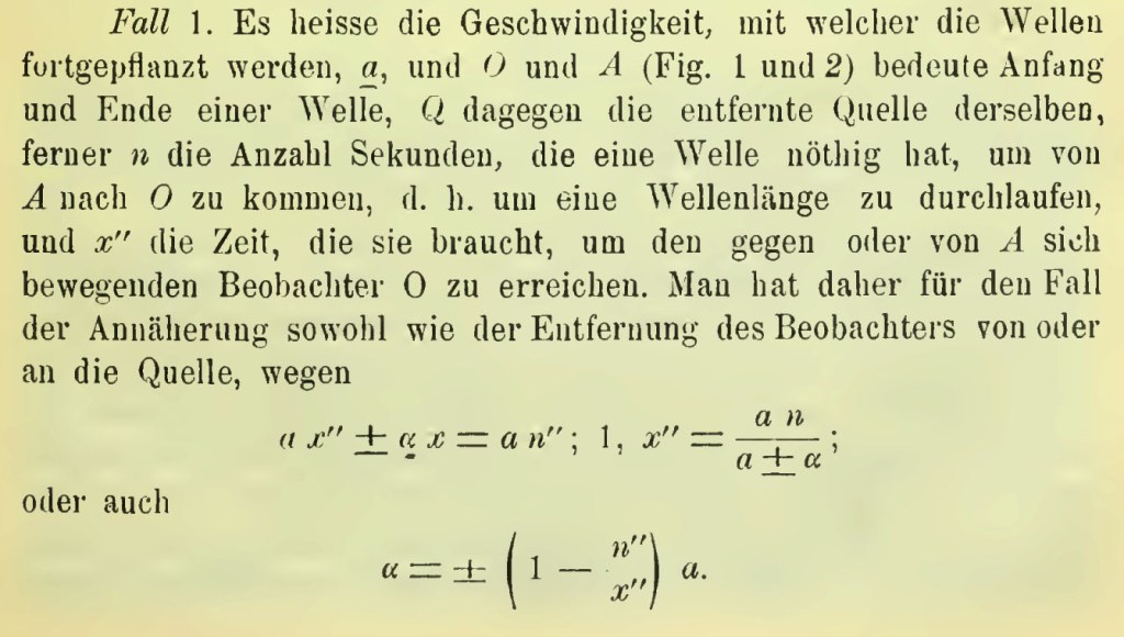
When Doppler proposed the shift in color of the light from stars in 1842 [1], depending on their motion towards or away from us, he may have been inspired by his walk to work every morning, watching the ripples on the surface of the Vltava River in Prague as the water slipped by the bridge piers. The drawings in his early papers look reminiscently like the patterns you see with compressed ripples on the upstream side of the pier and stretched out on the downstream side. Taking this principle to the night sky, Doppler envisioned that binary stars, where one companion was blue and the other was red, was caused by their relative motion. He could not have known at that time that typical binary star speeds were too small to cause this effect, but his principle was far more general, applying to all wave phenomena.
Six years later in 1848 [2], the French physicist Armand Hippolyte Fizeau, soon to be famous for making the first direct measurement of the speed of light, proposed the same principle, unaware of Doppler’s publications in German. As Fizeau was preparing his famous measurement, he originally worked with a spinning mirror (he would ultimately use a toothed wheel instead) and was thinking about what effect the moving mirror might have on the reflected light. He considered the effect of star motion on starlight, just as Doppler had, but realized that it was more likely that the speed of the star would affect the locations of the spectral lines rather than change the color. This is in fact the correct argument, because a Doppler shift on the black-body spectrum of a white or yellow star shifts a bit of the infrared into the visible red portion, while shifting a bit of the ultraviolet out of the visible, so that the overall color of the star remains the same, but Fraunhofer lines would shift in the process. Because of the independent development of the phenomenon by both Doppler and Fizeau, and because Fizeau was a bit clearer in the consequences, the effect is more accurately called the Doppler-Fizeau Effect, and in France sometimes only as the Fizeau Effect. Here in the US, we tend to forget the contributions of Fizeau, and it is all Doppler.

Doppler and Exoplanet Discovery
It is fitting that many of today’s applications of the Doppler effect are in astronomy. His original idea on binary star colors was wrong, but his idea that relative motion changes frequencies was right, and it has become one of the most powerful astrometric techniques in astronomy today. One of its important recent applications was in the discovery of extrasolar planets orbiting distant stars.
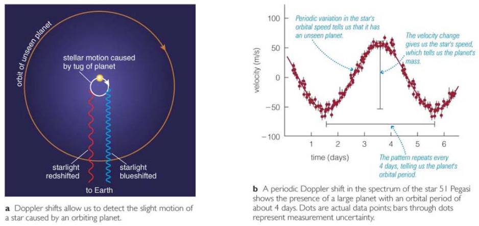
When a large planet like Jupiter orbits a star, the center of mass of the two-body system remains at a constant point, but the individual centers of mass of the planet and the star both orbit the common point. This makes it look like the star has a wobble, first moving towards our viewpoint on Earth, then moving away. Because of this relative motion of the star, the light can appear blueshifted caused by the Doppler effect, then redshifted with a set periodicity. This was observed by Queloz and Mayer in 1995 for the star 51 Pegasi, which represented the first detection of an exoplanet [3]. The duo won the Nobel Prize in 2019 for the discovery.
Doppler and Vera Rubins’ Galaxy Velocity Curves
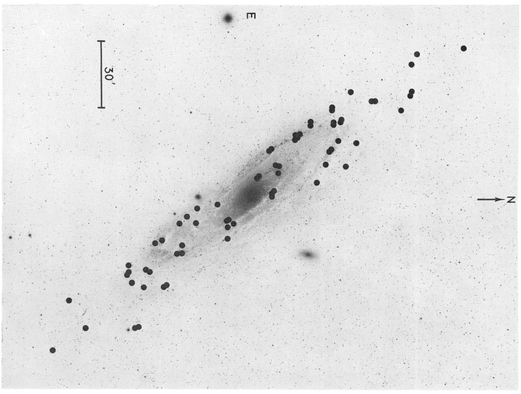
In the late 1960’s and early 1970’s Vera Rubin at the Carnegie Institution of Washington used newly developed spectrographs to use the Doppler effect to study the speeds of ionized hydrogen gas surrounding massive stars in individual galaxies [4]. From simple Newtonian dynamics it is well understood that the speed of stars as a function of distance from the galactic center should increase with increasing distance up to the average radius of the galaxy, and then should decrease at larger distances. This trend in speed as a function of radius is called a rotation curve. As Rubin constructed the rotation curves for many galaxies, the increase of speed with increasing radius at small radii emerged as a clear trend, but the stars farther out in the galaxies were all moving far too fast. In fact, they are moving so fast that they exceeded escape velocity and should have flown off into space long ago. This disturbing pattern was repeated consistently in one rotation curve after another for many galaxies.
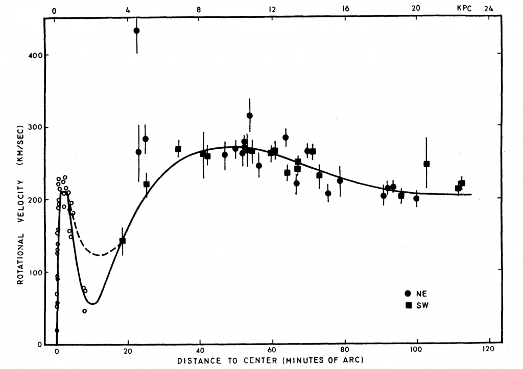

A simple fix to the problem of the rotation curves is to assume that there is significant mass present in every galaxy that is not observable either as luminous matter or as interstellar dust. In other words, there is unobserved matter, dark matter, in all galaxies that keeps all their stars gravitationally bound. Estimates of the amount of dark matter needed to fix the velocity curves is about five times as much dark matter as observable matter. In short, 80% of the mass of a galaxy is not normal. It is neither a perturbation nor an artifact, but something fundamental and large. The discovery of the rotation curve anomaly by Rubin using the Doppler effect stands as one of the strongest evidence for the existence of dark matter.
There is so much dark matter in the Universe that it must have a major effect on the overall curvature of space-time according to Einstein’s field equations. One of the best probes of the large-scale structure of the Universe is the afterglow of the Big Bang, known as the cosmic microwave background (CMB).
Doppler and the Big Bang
The Big Bang was astronomically hot, but as the Universe expanded it cooled. About 380,000 years after the Big Bang, the Universe cooled sufficiently that the electron-proton plasma that filled space at that time condensed into hydrogen. Plasma is charged and opaque to photons, while hydrogen is neutral and transparent. Therefore, when the hydrogen condensed, the thermal photons suddenly flew free and have continued unimpeded, continuing to cool. Today the thermal glow has reached about three degrees above absolute zero. Photons in thermal equilibrium with this low temperature have an average wavelength of a few millimeters corresponding to microwave frequencies, which is why the afterglow of the Big Bang got its name: the Cosmic Microwave Background (CMB).
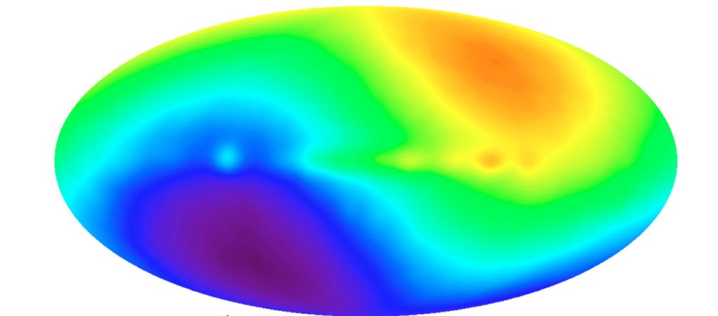
Not surprisingly, the CMB has no preferred reference frame, because every point in space is expanding relative to every other point in space. In other words, space itself is expanding. Yet soon after the CMB was discovered by Arno Penzias and Robert Wilson (for which they were awarded the Nobel Prize in Physics in 1978), an anisotropy was discovered in the background that had a dipole symmetry caused by the Doppler effect as the Solar System moves at 368±2 km/sec relative to the rest frame of the CMB. Our direction is towards galactic longitude 263.85o and latitude 48.25o, or a bit southwest of Virgo. Interestingly, the local group of about 100 galaxies, of which the Milky Way and Andromeda are the largest members, is moving at 627±22 km/sec in the direction of galactic longitude 276o and latitude 30o. Therefore, it seems like we are a bit slack in our speed compared to the rest of the local group. This is in part because we are being pulled towards Andromeda in roughly the opposite direction, but also because of the speed of the solar system in our Galaxy.
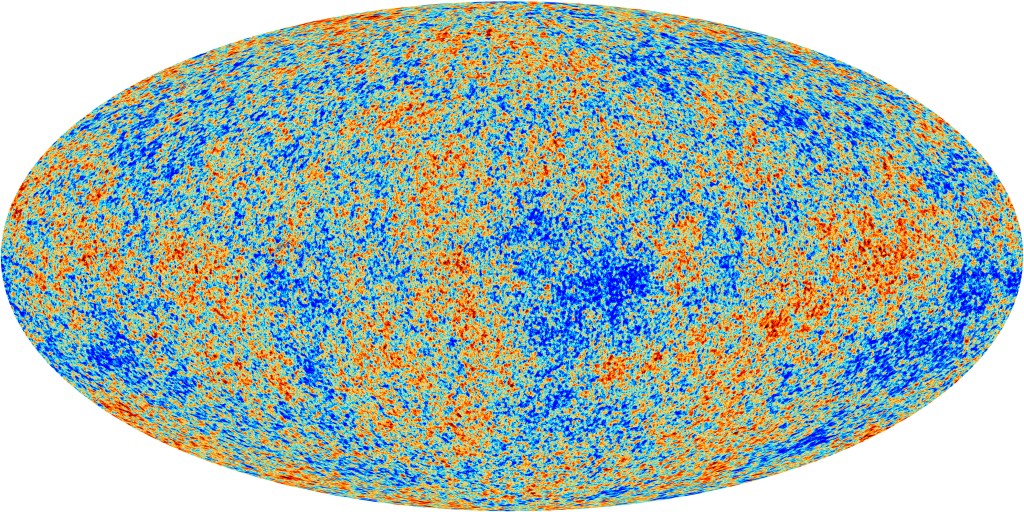
Aside from the dipole anisotropy, the CMB is amazingly uniform when viewed from any direction in space, but not perfectly uniform. At the level of 0.005 percent, there are variations in the temperature depending on the location on the sky. These fluctuations in background temperature are called the CMB anisotropy, and they help interpret current models of the Universe. For instance, the average angular size of the fluctuations is related to the overall curvature of the Universe. This is because, in the early Universe, not all parts of it were in communication with each other. This set an original spatial size to thermal discrepancies. As the Universe continued to expand, the size of the regional variations expanded with it, and the sizes observed today would appear larger or smaller, depending on how the universe is curved. Therefore, to measure the energy density of the Universe, and hence to find its curvature, required measurements of the CMB temperature that were accurate to better than a part in 10,000.
Equivalently, parts of the early universe had greater mass density than others, causing the gravitational infall of matter towards these regions. Then, through the Doppler effect, light emitted (or scattered) by matter moving towards these regions contributes to the anisotropy. They contribute what are known as “Doppler peaks” in the spatial frequency spectrum of the CMB anisotropy.
The examples discussed in this blog (exoplanet discovery, galaxy rotation curves, and cosmic background) are just a small sampling of the many ways that the Doppler effect is used in Astronomy. But clearly, Doppler has played a key role in the long history of the universe.
By David D. Nolte, Jan. 23, 2022
References:
[1] C. A. DOPPLER, “Über das farbige Licht der Doppelsterne und einiger anderer Gestirne des Himmels (About the coloured light of the binary stars and some other stars of the heavens),” Proceedings of the Royal Bohemian Society of Sciences, vol. V, no. 2, pp. 465–482, (Reissued 1903) (1842)
[2] H. Fizeau, “Acoustique et optique,” presented at the Société Philomathique de Paris, Paris, 1848.
[3] M. Mayor and D. Queloz, “A JUPITER-MASS COMPANION TO A SOLAR-TYPE STAR,” Nature, vol. 378, no. 6555, pp. 355-359, Nov (1995)
[4] Rubin, Vera; Ford, Jr., W. Kent (1970). “Rotation of the Andromeda Nebula from a Spectroscopic Survey of Emission Regions”. The Astrophysical Journal. 159: 379
Further Reading
D. D. Nolte, “The Fall and Rise of the Doppler Effect,” Physics Today, vol. 73, no. 3, pp. 31-35, Mar (2020)
M. Tegmark, “Doppler peaks and all that: CMB anisotropies and what they can tell us,” in International School of Physics Enrico Fermi Course 132 on Dark Matter in the Universe, Varenna, Italy, Jul 25-Aug 04 1995, vol. 132, in Proceedings of the International School of Physics Enrico Fermi, 1996, pp. 379-416

[…] perpendicular to the line of sight to an observer. This effect had not been predicted either by Christian Doppler (1803 – 1853) or by Woldemar Voigt (1850 – […]
LikeLike