

One of the most important conclusions from chaos theory is that not all random-looking processes are actually random. In deterministic chaos, structures such as strange attractors are not random at all but are fractal structures determined uniquely by the dynamics. But sometimes, in nature, processes really are random, or at least have to be treated as such because of their complexity. Brownian motion is a perfect example of this. At the microscopic level, the jostling of the Brownian particle can be understood in terms of deterministic momentum transfers from liquid atoms to the particle. But there are so many liquid particles that their individual influences cannot be directly predicted. In this situation, it is more fruitful to view the atomic collisions as a stochastic process with well-defined physical parameters and then study the problem statistically. This is what Einstein did in his famous 1905 paper that explained the statistical physics of Brownian motion.
Then there is the middle ground between deterministic mechanics and stochastic mechanics, where complex dynamics gains a stochastic component. This is what Paul Langevin did in 1908 when he generalized Einstein.
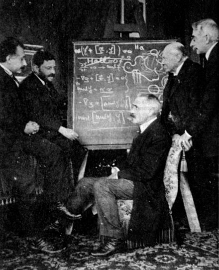
Paul Langevin
Paul Langevin (1872 – 1946) had the fortune to stand at the cross-roads of modern physics, making key contributions, while serving as a commentator expanding on the works of the giants like Einstein and Lorentz and Bohr. He was educated at the École Normale Supérieure and at the Sorbonne with a year in Cambridge studying with J. J. Thompson. At the Sorbonne he worked in the laboratory of Jean Perrin (1870 – 1942) who received the Nobel Prize in 1926 for the experimental work on Brownian motion that had set the stage for Einstein’s crucial analysis of the problem confirming the atomic nature of matter.
Langevin received his PhD in 1902 on the topic of x-ray ionization of gases and was appointed as a lecturer at the College de France to substitute in for Éleuthère Mascart (who was an influential French physicist in optics). In 1905 Langevin published several papers that delved into the problems of Lorentz contraction, coming very close to expressing the principles of relativity. This work later led Einstein to say that, had he delayed publishing his own 1905 paper on the principles of relativity, then Langevin might have gotten there first [1].
Also in 1905, Langevin published his most influential work, providing the theoretical foundations for the physics of paramagnetism and diamagnetism. He was working closely with Pierre Curie whose experimental work on magnetism had established the central temperature dependence of the phenomena. Langevin used the new molecular model of matter to derive the temperature dependence as well as the functional dependence on magnetic field. One surprising result was that only the valence electrons, moving relativistically, were needed to contribute to the molecular magnetic moment. This later became one of the motivations for Bohr’s model of multi-electron atoms.
Langevin suffered personal tragedy during World War II when the Vichy government arrested him because of his outspoken opposition to fascism. He was imprisoned and eventually released to house arrest. In 1942, his son-in-law was executed by the Nazis, and in 1943 his daughter was sent to Auschwitz. Fearing for his own life, Langevin escaped to Switzerland. He returned shortly after the liberation of Paris and was joined after the end of the war by his daughter who had survived Auschwitz and later served in the Assemblée Consultative as a communist member. Langevin passed away in 1946 and received a national funeral. His remains lie today in the Pantheon.
The Langevin Equation
In 1908, Langevin realized that Einstein’s 1905 theory on Brownian motion could be simplified while at the same time generalized. Langevin introduced a new quantity into theoretical physics—the stochastic force [2]. With this new theoretical tool, he was able to work with diffusing particles in momentum space as dynamical objects with inertia buffeted by random forces, providing a Newtonian formulation for short-time effects that were averaged out and lost in Einstein’s approach.
Stochastic processes are understood by considering a dynamical flow that includes a random function. The resulting set of equations are called the Langevin equation, namely

where fa is a set of N regular functions, and σa is the standard deviation of the a-th process out of N. The stochastic functions ξa are in general non-differentiable but are integrable. They have zero mean, and no temporal correlations. The solution is an N-dimensional trajectory that has properties of a random walk superposed on the dynamics of the underlying mathematical flow.
As an example, take the case of a particle moving in a one-dimensional potential, subject to drag and to an additional stochastic force

where γ is the drag coefficient, U is a potential function and B is the velocity diffusion coefficient. The second term in the bottom equation is the classical force from a potential function, while the third term is the stochastic force. The crucial point is that the stochastic force causes jumps in velocity that integrate into displacements, creating a random walk superposed on the deterministic mechanics.

Random Walk in a Harmonic Potential
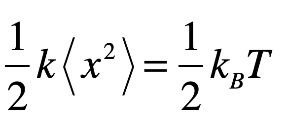
Diffusion of a particle in a weak harmonic potential is equivalent to a mass on a weak spring in a thermal bath. For short times, the particle motion looks like a random walk, but for long times, the mean-squared displacement must satisfy the equipartition relation
The Langevin equation is the starting point of motion under a stochastic force F’
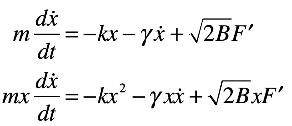
where the second equation has been multiplied through by x. For a spherical particle of radius a, the viscous drag factor is
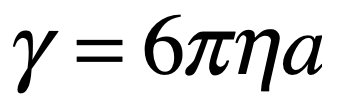
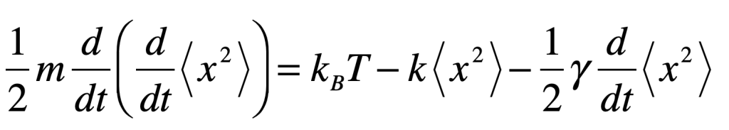
and η is the viscosity. The term on the left of the dynamical equation can be rewritten to give

It is then necessary to take averages. The last term on the right vanishes because of the random signs of xF’. However, the buffeting from the random force can be viewed as arising from an effective temperature. Then from equipartition on the velocity

this gives
Making the substitution y = <x2> gives
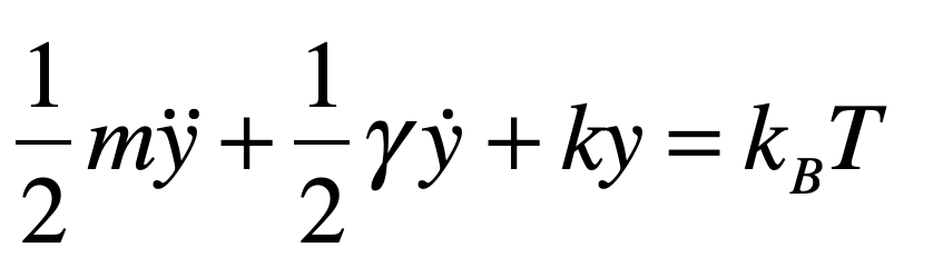
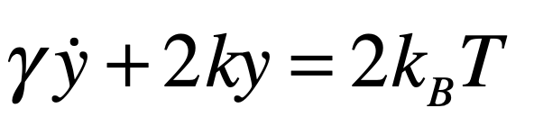
which is the dynamical equation for a particle in a harmonic potential subject to a constant effective force kBT. For small objects in viscous fluids, the inertial terms are negligible relative to the other terms (see Life at small Reynolds Number [3]), so the dynamic equation is
with the general solution
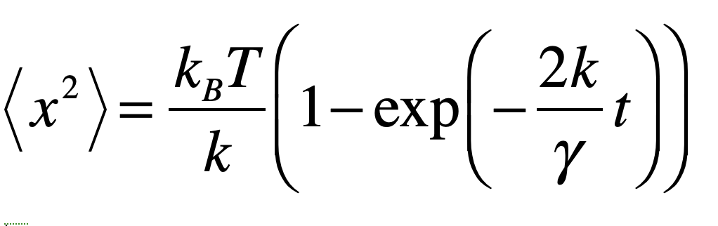
For short times, this is expanded by the Taylor series to
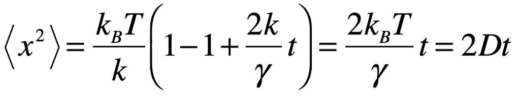
This solution at short times describes a diffusing particle (Fickian behavior) with a diffusion coefficient D. However, for long times the solution asymptotes to an equipartition value of <x2> = kBT/k. In the intermediate time regime, the particle is walking randomly, but the mean-squared displacement is no longer growing linearly with time.
Constrained motion shows clear saturation to the size set by the physical constraints (equipartition for an oscillator or compartment size for a freely diffusing particle [4]). However, if the experimental data do not clearly extend into the saturation time regime, then the fit to anomalous diffusion can lead to exponents that do not equal unity. This is illustrated in Fig. 3 with asymptotic MSD compared with the anomalous diffusion equation fit for the exponent β. Care must be exercised in the interpretation of the exponents obtained from anomalous diffusion experiments. In particular, all constrained motion leads to subdiffusive interpretations if measured at intermediate times.

Random Walk in a Double Potential
The harmonic potential has well-known asymptotic dynamics which makes the analytic treatment straightforward. However, the Langevin equation is general and can be applied to any potential function. Take a double-well potential as another example
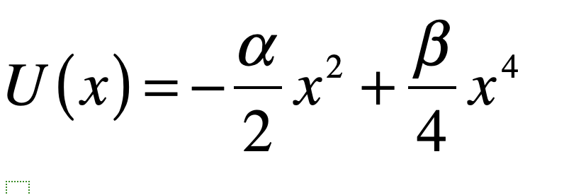
The resulting Langevin equation can be solved numerically in the presence of random velocity jumps. A specific stochastic trajectory is shown in Fig. 4 that applies discrete velocity jumps using a normal distribution of jumps of variance 2B. The notable character of this trajectory, besides the random-walk character, is the ability of the particle to jump the barrier between the wells. In the deterministic system, the initial condition dictates which stable fixed point would be approached. In the stochastic system, there are random fluctuations that take the particle from one basin of attraction to the other.

The stochastic long-time probability distribution p(x,v) in Fig. 5 introduces an interesting new view of trajectories in state space that have a different character than typical state-space flows. If we think about starting a large number of systems with the same initial conditions, and then letting the stochastic dynamics take over, we can define a time-dependent probability distribution p(x,v,t) that describes the likely end-positions of an ensemble of trajectories on the state plane as a function of time. This introduces the idea of the trajectory of a probability cloud in state space, which has a strong analogy to time-dependent quantum mechanics. The Schrödinger equation can be viewed as a diffusion equation in complex time, which is the basis of a technique known as quantum Monte Carlo that solves for ground state wave functions using concepts of random walks. This goes beyond the topics of classical mechanics, and it shows how such diverse fields as econophysics, diffusion, and quantum mechanics can share common tools and language.

Stochastic Chaos
“Stochastic Chaos” sounds like an oxymoron. “Chaos” is usually synonymous with “deterministic chaos”, meaning that every next point on a trajectory is determined uniquely by its previous location–there is nothing random about the evolution of the dynamical system. It is only when one looks at long times, or at two nearby trajectories, that non-repeatable and non-predictable behavior emerges, so there is nothing stochastic about it.
On the other hand, there is nothing wrong with adding a stochastic function to the right-hand side of a deterministic flow–just as in the Langevin equation. One question immediately arises: if chaos has sensitivity to initial conditions (SIC), wouldn’t it be highly susceptible to constant buffeting by a stochastic force? Let’s take a look!
To the well-known Rössler model, add a stochastic function to one of the three equations,
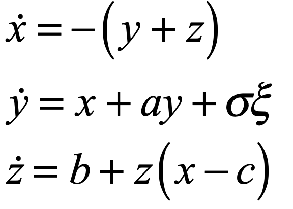
in this case to the y-dot equation. This is just like the stochastic term in the random walks in the harmonic and double-well potentials. The solution is shown in Fig. 6. In addition to the familiar time-series of the Rössler model, there are stochastic jumps in the y-variable. An x-y projection similarly shows the familiar signature of the model, and the density of trajectory points is shown in the density plot on the right. The rms jump size for this simulation is approximately 10%.

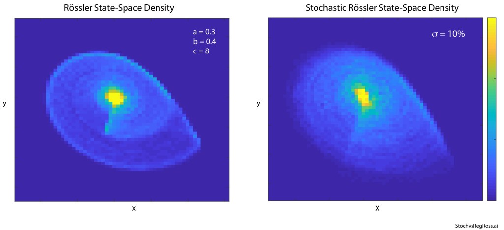
Now for the supposition that because chaos has sensitivity to initial conditions that it should be highly susceptible to stochastic contributions–the answer can be seen in Fig. 7 in the state-space densities. Other than a slightly more fuzzy density for the stochastic case, the general behavior of the Rössler strange attractor is retained. The attractor is highly stable against the stochastic fluctuations. This demonstrates just how robust deterministic chaos is.
On the other hand, there is a saddle point in the Rössler dynamics a bit below the lowest part of the strange attractor in the figure, and if the stochastic jumps are too large, then the dynamics become unstable and diverge. A hint at this is already seen in the time series in Fig. 6 that shows the nearly closed orbit that occurs transiently at large negative y values. This is near the saddle point, and this trajectory is dangerously close to going unstable. Therefore, while the attractor itself is stable, anything that drives a dynamical system to a saddle point will destabilize it, so too much stochasticity can cause a sudden destruction of the attractor.
• Parts of this blog were excerpted from D. D. Nolte, Optical Interferometry for Biology and Medicine. Springer, 2012, pp. 1-354 and D. D. Nolte, Introduction to Modern Dynamics. Oxford, 2015 (first edition).
[1] A. Einstein, “Paul Langevin” in La Pensée, 12 (May-June 1947), pp. 13-14.
[2] D. S. Lemons and A. Gythiel, “Paul Langevin’s 1908 paper ”On the theory of Brownian motion”,” American Journal of Physics, vol. 65, no. 11, pp. 1079-1081, Nov (1997)
[3] E. M. Purcell, “Life at Low Reynolds-Number,” American Journal of Physics, vol. 45, no. 1, pp. 3-11, (1977)
[4] Ritchie, K., Shan, X.Y., Kondo, J., Iwasawa, K., Fujiwara, T., Kusumi, A.: Detection of non- Brownian diffusion in the cell membrane in single molecule tracking. Biophys. J. 88(3), 2266–2277 (2005)
