

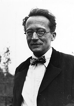
By the middle of 1925, a middle-aged Erwin Schrödinger was casting about, bogged down in mid career, looking for something significant to say about the rapidly accelerating field of quantum theory. He was known for his breadth of knowledge, and for his belief in his own creative genius [1], but a grand synthesis had so far eluded him.
Einsteinian Gas Theory
In the middle of the year, Schrödinger was deep analyzing two papers recently published by Einstein (Sept. 1924 and Feb. 1925) on the quantum properties of ideal gases where Einstein applied the new statistical theory of Bose to the counting of states in a volume of the gas [2]. One of the intriguing discoveries made by Einstein in those papers was a close analogy between the fluctuation of gas numbers and the interference of waves. He stated:
‘I believe that this is more than a mere analogy; de Broglie has shown in a very important work how a (scalar) wave field can be coordinated with a material particle or a system of material particles’
referring to de Broglie’s thesis work of 1924 that associated a wave-like property to mass. Einstein had been the first to attribute a wave-particle duality to the quantum phenomenon of black-body radiation, giving a lecture in Salzburg, Austria, in 1909 showing relationships between the particle-like and the wave-like properties of the radiation, and he found similar behavior in the properties of monatomic ideal gases, though his derivations were purely statistical.
Schrödinger was suspicious of the “unnatural” way of counting states used by Einstein and Bose for the gas, and he sought a more “natural” way of explaining how the elements of phase space were filled. It struck him that, just as Planck’s black-body radiation spectrum could be derived by assuming discrete standing-wave modes for the electromagnetic radiation, then perhaps the behavior of ideal gases could be obtained using a similar approach. He and Einstein exchanged several letters about this idea as Schrödinger dug deeper into de Broglie’s theory.
The Zurich Seminar
At that time, Schrödinger was in the Chair of Theoretical Physics at the University of Zurich, holding the same chair that Einstein had held 15 years earlier. Following Einstein, the chair had been occupied by Max von Laue and then by Peter Debye who moved to the ETH in Zurich. Debye organized a joint seminar between the University and ETH that was a hot social gathering of physicists and physical chemists, discussing the latest developments in atomic and quantum science.
In November of 2025, Debye, who probably knew about the Einstein-Schrödinger discussion on de Broglie, asked Schrödinger to give a seminar on de Broglie’s theory to the group. A young Felix Bloch, who was a graduate student at that time, recalled hearing Debye say something like
“Schrödinger, you are not working right now on very important problems anyway. Why don’t you tell us sometime about that thesis of de Broglie, which seems to have attracted some attention?”[3]
Schrödinger gave the overview seminar in early December, showing how the Bohr-Sommerfeld quantization conditions could be explained as standing waves using de Broglie’s theory, but Bloch recalled Debye was unimpressed, saying that de Broglie’s way of talking was “childish” and that what was needed for a proper physics theory was a wave equation.
This exchange between Schrödinger and Debye was recalled only in later years, and there is debate about what exactly was said and what effect it had on Schrödinger. From Schrödinger’s letters to friends, it is clear that he was already well into his investigations of wavelike properties of matter when Debye asked him to give the seminar. Furthermore, he had already tried to construct wave packets using superpositions of phase waves propagating along Bohr-Sommerfeld elliptical orbits but had been led to ugly caustics when he tried to apply the packets to the hydrogen atom [4]. Therefore, although Debye was probably not the source of Schrödinger’s interest in de Broglie, it is possible that Debye’s quip about “childishness” may have spurred Schrödinger to find a wave equation subject to boundary conditions rather than working with packets following ray paths.
The Christmas Breakthrough
By this time, Christmas was approaching and Schrödinger arranged to take a vacation away from his family to the Swiss Alpine village of Arosa, and given his unconventional belief in the link between personal pleasure and genius, he did not go alone. There is no record of what transpired, and no record of which mistress was with him on this particular trip, nor how she spent her time while he worked on his theory, but two days after Christmas he wrote a letter to the physicist Willy Wien saying
“At the moment I am struggling with a new atomic theory. If only I knew more mathematics! I am very optimistic about this thing, and expect that, if only I can . . . solve it, it will be very beautiful.. . . I hope that I can soon report in a little more detailed and understandable way about the matter. At present I must learn a little mathematics in order to completely solve the vibration problem …”[5]
He had uncovered his first wave equation. When he returned to Zurich, he enlisted the help of his friend, the mathematician Hermann Weyl at the University in Zurich, and Schrödinger had his first eigenfrequencies for hydrogen. But they were wrong!
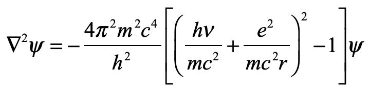
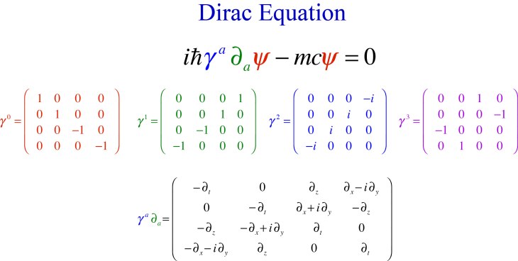
The theory of de Broglie was fundamentally a relativistic theory, motivated by mapping the behavior of matter onto the behavior of light. Therefore, Schrödinger’s first attempt was also relativistic, equivalent to the Klein-Gordon equation. But there was no clear understanding of electron spin at that time, even though it had been established as a fundamental property of the electron. It was only several years later when Dirac correctly accounted for electron spin in a relativistic wave equation.
The Schrödinger Wave Equation
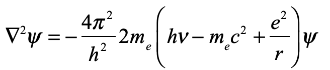
Convinced that he was onto something big, and unwilling to fail, despite his failure to obtain correct values for hydrogen, Schrödinger went back to first principles, to the classical theory of Hamiltonian mechanics, identifying Hamilton’s characteristic function with the phase of an electron wave and deriving a non-relativistic equation using variational principles subject to boundary conditions. The eigenvalues of this new equation, when applied to hydrogen, matched the Bohr spectrum perfectly!
It had been only a few weeks since Schrödinger had given his previous seminar to the Zurich group, but in January he gave his update, probably given with some degree of satisfaction, having Debye in attendance, showing his now-famous wave equation and the agreement with experiment. Schrödinger wrote up his theory and results and submitted his paper on January 27, 1926, to Annalen der Physik [6].
Schrödinger had been known, but not as a forefront thinker, despite what he believed about himself. Now he was a forefront thinker, vindicating his beliefs but not always on the right track. He continued his unconventional lifestyle, marginalizing him socially, and he resisted Max Born’s and Niels Bohr’s probabilistic interpretations of the meaning of his own quantum wavefunction, marginalizing him professionally. Yet his breakthrough gave him a platform, and his skeptical reactions to his colleague’s successes helped illuminate the nature of the new physics (“Schrödinger’s Cat” [7]) through the decades to follow.
Bibliography
A very large body of historical work exists on the discovery of the Schrödinger equation, partially fueled by the lack of first-person accounts on how he achieved it. There has been a lot of speculation and a lot of sleuthing to uncover his path of discovery. Several accounts differ mainly in the timing of when he derived his equations, although all agree on the sequence: that the relativistic equation preceded the non-relativistic one. Here is a small sampling of the literature:
• Hanle, P. A. (1977). “The Coming of Age of Erwin Schrödinger: His Quantum Statistics of Ideal Gases.” Archive for History of Exact Sciences, 17(2), 165–192. DOI: 10.1007/BF00328532.
• Hanle, P. A. (1979). “The Schrödinger‐Einstein correspondence and the sources of wave mechanics.” American Journal of Physics, 47(7), 644–648. DOI: 10.1119/1.11587.
• Mehra, Jagdish. “Erwin Schrödinger and the Rise of Wave Mechanics. II. The Creation of Wave Mechanics.” Foundations of Physics, vol. 17, no. 12, 1987, pp. 1141-1188.
• Renn, J. (2013). “Schrödinger and the Genesis of Wave Mechanics.” In W. L. Reiter & J. Yngvason (Eds.), Erwin Schrödinger – 50 Years After (pp. 9–36). Zurich: European Mathematical Society. DOI: 10.4171/121-1/2.
• Wessels, L. (1979). “Schrödinger’s Route to Wave Mechanics.” Studies in History and Philosophy of Science Part A, 10(4), 311–340.
Notes
[1] He led an unconventional lifestyle (some would say emotionally predatory) based on his belief in the personal origins of genius. Although this behavior presented significant social barriers to his career, he refused to abandon it.
[2] A. Enstein, ‘Quantentheorie des einatomigen idealen Gases’, Preuss. Ak. Wiss. Sitzb. (1924) pp. 261 – 267, and (1925), pp. 3-14.
[3] Quoted in Mehra, pg. 1150
[4] Mehra, pg. 1147
[5] Wessels, pg. 328
[6] Schrödinger, Erwin. “Quantisierung als Eigenwertproblem (Erste Mitteilung).” Annalen Der Physik, vol. 384, no. 4, 1926, pp. 361-376.
[7] Schrödinger, E. (1935). “Die gegenwärtige Situation in der Quantenmechanik.” Naturwissenschaften 23: 807–812, 823–828, 844–849. Schrödinger, E. (1980). “The Present Situation in Quantum Mechanics: A Translation of Schrödinger’s ‘Cat Paradox’ Paper.” Proceedings of the American Philosophical Society 124 (5): 323–338. (Translated by J. D. Trimmer).


.jpg)