Fractals, those telescoping self-similar filigree meshes that marry mathematics and art, have become so mainstream, that they are even mentioned in the theme song of Disney’s 2013 mega-hit, Frozen.
My power flurries through the air into the ground My soul is spiraling in frozen fractals all around And one thought crystallizes like an icy blast I’m never going back, the past is in the past
Let it Go, by Idina Menzel (Frozen, Disney 2013)
But not all fractals are cut from the same cloth. Some are thin and some are fat. The thin ones are the ones we know best, adorning the cover of books and magazines. But the fat ones may be more common and may play important roles, such as in the stability of celestial orbits in a many-planet neighborhood, or in the stability and structure of Saturn’s rings.
To get a handle on fat fractals, we will start with a familiar thin one, the zero-measure Cantor set.
The Zero-Measure Cantor Set
The famous one-third Cantor set is often the first fractal that you encounter in any introduction to fractals. (See my blog on a short history of fractals.) It lives on a one-dimensional line, and its iterative construction is intuitive and simple.
Start with a long thin bar of unit length. Then remove the middle third, leaving the endpoints. This leaves two identical bars of one-third length each. Next, remove the open middle third of each of these, again leaving the endpoints, leaving behind section pairs of one-nineth length. Then repeat ad infinitum. The points of the line that remain–all those segment endpoints–are the Cantor set.
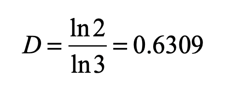
Fig. 1 Construction of the 1/3 Cantor set by removing 1/3 segments at each level, and leaving the endpoints of each segment. The resulting set is a dust of points with a fractal dimension D = ln(2)/ln(3) = 0.6309.
The Cantor set has a fractal dimension that is easily calculated by noting that at each stage there are two elements (N = 2) that divided by three in size (b = 3). The fractal dimension is then
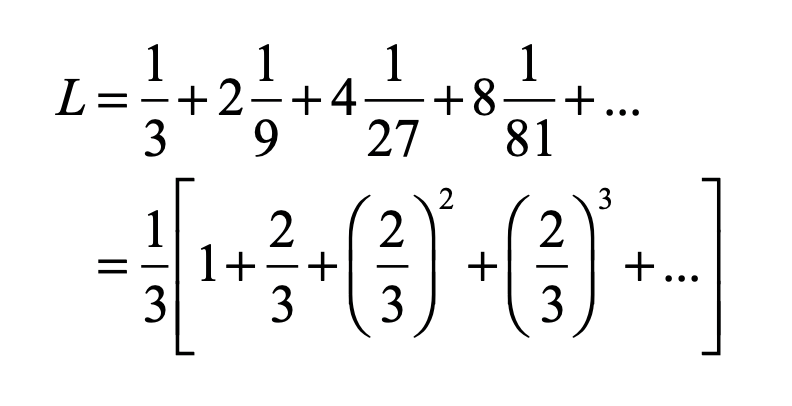
It is easy to prove that the collection of points of the Cantor set have no length because all of the length was removed.
For instance, at the first level, one third of the length was removed. At the second level, two segments of one-nineth length were removed. At the third level, four segments of one-twenty-sevength length were removed, and so on. Mathematically, this is
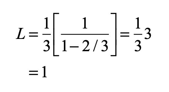
The infinite series in the brackets is a binomial series with the simple solution
Therefore, all the length has been removed, and none is left to the Cantor set, which is simply a collection of all the endpoints of all the segments that were removed.
The Cantor set is said to have a Lebesgue measure of zero. It behaves as a dust of isolated points.
A close relative of the Cantor set is the Sierpinski Carpet which is the two-dimensional analog. It begins with a square of unit side, then the middle third is removed (one nineth of the three-by-three array of square of one-third side), and so on.
Fig. 2 A regular Sierpinski Carpet with fractal dimension D = ln(8)/ln(3) = 1.8928.
The resulting Sierpinski Carpet has zero Lebesgue measure, just like the Cantor dust, because all the area has been removed.
There are also random Sierpinski Carpets as the sub-squares are removed from random locations.
Fig. 3 A random Sierpinski Carpet with fractal dimension D = ln(8)/ln(3) = 1.8928.
These fractals are “thin”, so-called because they are dusts with zero measure.
But the construction was constructed just so, such that the sum over all the removed sub-lengths summed to unity. What if less material had been taken at each step? What happens?
Fat Fractals
Instead of taking one-third of the original length, take instead one-fourth. But keep the one-third scaling level-to-level, as for the original Cantor Set.
Fig. 4 A “fat” Cantor fractal constructed by removing 1/4 of a segment at each level instead of 1/3.
The total length removed is
Therefore, three fourths of the length was removed, leaving behind one fourth of the material. Not only that, but the material left behind is contiguous—solid lengths. At each level, a little bit of the original bar remains, and still remains at the next level and the next. Therefore, it is said to have a Lebesgue measure of unity. This construction leads to a “fat” fractal.
Fig. 5 Fat Cantor fractal showing the original Cantor 1/3 set (in black) and the extra contiguous segments (in red) that give the set a Lebesgue measure equal to one.
Looking at Fig. 5, it is clear that the original Cantor dust is still present as the black segments interspersed among the red parts of the bar that are contiguous. But when two sets are added that have different “dimensions”, then the combined set has the larger dimension of the two, which is one-dimensional in this case. The fat Cantor set is one dimensional. One can still study its scaling properties, leading to another type of dimension known as an exterior measure [1], but where do such fat fractals occur? Why do they matter?
One answer is that they lie within the oddly named “Arnold Tongues” that arise in the study of synchronization and resonance connected to the stability of the solar system and the safety of its inhabitants.
Arnold Tongues
The study of synchronization explores and explains how two or more non-identical oscillators can lock themselves onto a common shared oscillation. For two systems to synchronize requires autonomous oscillators (like planetary orbits) with a period-dependent interaction (like gravity). Such interactions are “resonant” when the periods of the two orbits are integer ratios of each other, like 1:2 or 2:3. Such resonances ensure that there is a periodic forcing caused by the interaction that is some multiple of the orbital period. Think of tapping a rotating bicycle wheel twice per cycle or three times per cycle. Even if you are a little off in your timing, you can lock the tire rotation rate to a multiple of your tapping frequency. But if you are too far off on your timing, then the wheel will turn independently of your tapping.
Because rational ratios of integers are plentiful, there can be an intricate interplay between locked frequencies and unlocked frequencies. When the rotation rate is close to a resonance, then the wheel can frequency-lock to the tapping. Plotting the regions where the wheel synchronizes or not as a function of the frequency ratio and also as a function of the strength of the tapping leads to one of the iconic images of nonlinear dynamics: the Arnold tongue diagram.
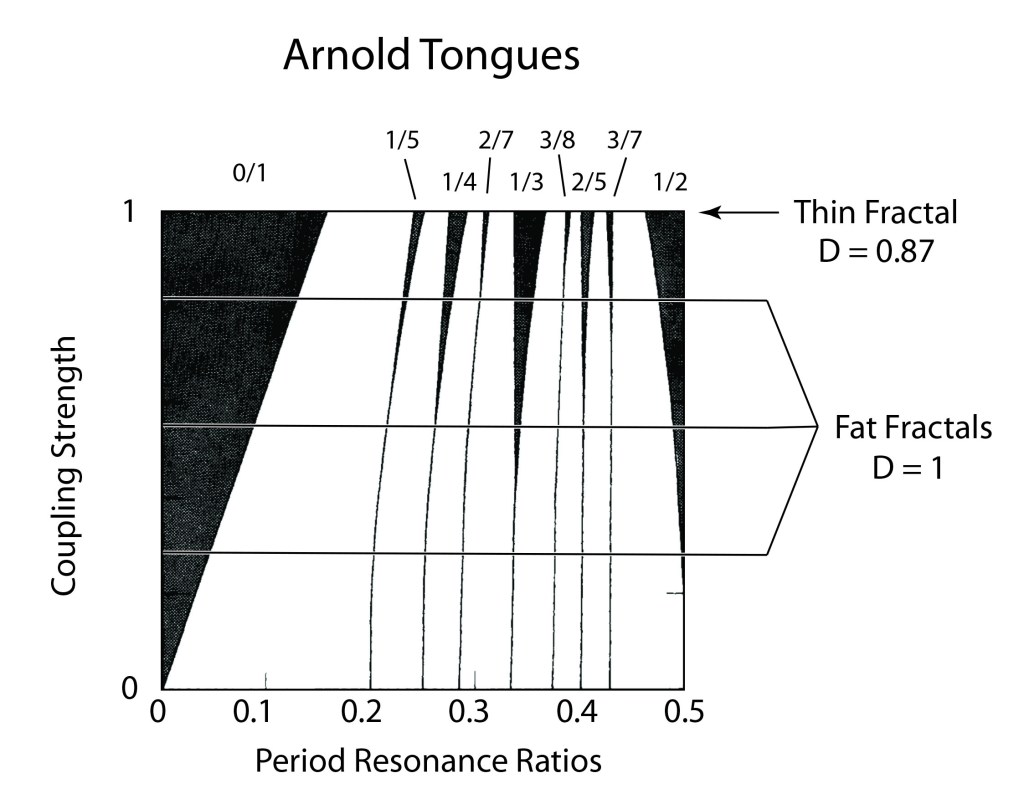
Fig. 6 Arnold tongue diagram, showing the regions of frequency locking (black) at rational resonances as a function of coupling strength. At unity coupling strength, the set outside frequency-locked regions is fractal with D = 0.87. For all smaller coupling, a set along a horizontal is a fat fractal with topological dimension D = 1. The white regions are “ergodic”, as the phase of the oscillator runs through all possible values.
The Arnold tongues in Fig. 6 are the frequency locked regions (black) as a function of frequency ratio and coupling strength g. The black regions correspond to rational ratios of frequencies. For g = 1, the set outside frequency-locked regions (the white regions are “ergodic”, as the phase of the oscillator runs through all possible values) is a thin fractal with D = 0.87. For g < 1, the sets outside the frequency locked regions along a horizontal (at constant g) are fat fractals with topological dimension D = 1. For fat fractals, the fractal dimension is irrelevant, and another scaling exponent takes on central importance.
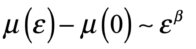
The Lebesgue measure μ of the ergodic regions (the regions that are not frequency locked) is a function of the coupling strength varying from μ = 1 at g = 0 to μ = 0 at g = 1. When the pattern is coarse-grained at a scale ε, then the scaling of a fat fractal is
where β is the scaling exponent that characterizes the fat fractal.
From numerical studies [2] there is strong evidence that β = 2/3 for the fat fractals of Arnold Tongues.
The Rings of Saturn
Arnold Tongues arise in KAM theory on the stability of the solar system (See my blog on KAM and how number theory protects us from the chaos of the cosmos). Fortunately, Jupiter is the largest perturbation to Earth’s orbit, but its influence, while non-zero, is not enough to seriously affect our stability. However, there is a part of the solar system where rational resonances are not only large but dominant: Saturn’s rings.
Saturn’s rings are composed of dust and ice particles that orbit Saturn with a range of orbital periods. When one of these periods is a rational fraction of the orbital period of a moon, then a resonance condition is satisfied. Saturn has many moons, producing highly corrugated patterns in Saturn’s rings at rational resonances of the periods.
Fig. 7 A close up of Saturn’s rings shows a highly detailed set of bands. Particles at a given radius have a given period (set by Kepler’s third law). When the period of dust particles in the ring are an integer ratio of the period of a “shepherd moon”, then a resonance can drive density rings. [See image reference.]
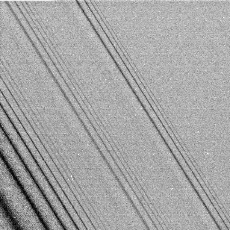
The moons Janus and Epithemeus share an orbit around Saturn in a rare 1:1 resonance in which they swap positions every four years. Their combined gravity excites density ripples in Saturn’s rings, photographed by the Cassini spacecraft and shown in Fig. 8.
Fig. 8 Cassini spacecraft photograph of density ripples in Saturns rings caused by orbital resonance with the pair of moons Janus and Epithemeus.
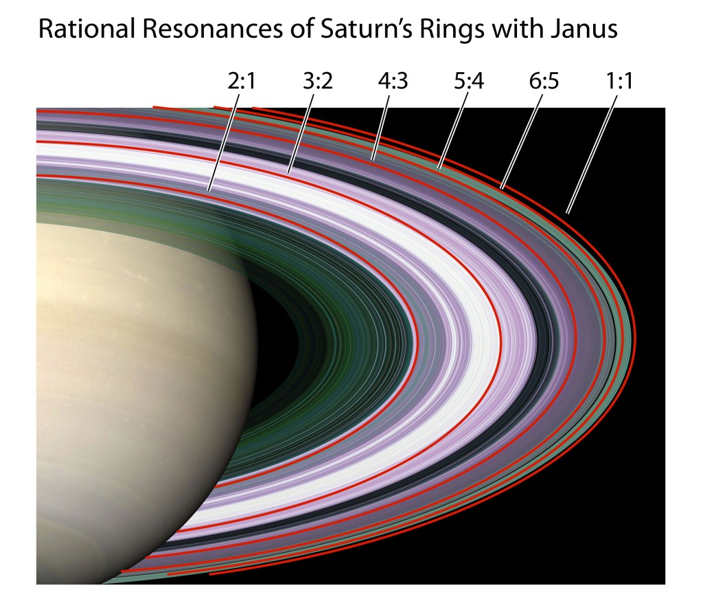
One Canadian astronomy group converted the resonances of the moon Janus into a musical score to commenorate Cassini’s final dive into the planet Saturn in 2017. The Janus resonances are shown in Fig. 9 against the pattern of Saturn’s rings.
Fig. 7 Rational resonances for subrings of Saturn relative to its moon Janus.
Saturn’s rings, orbital resonances, Arnold tongues and fat fractals provide a beautiful example of the power of dynamics to create structure, and the primary role that structure plays in deciphering the physics of complex systems.
By David D. Nolte, Nov. 28, 2023
References:
[1] C. Grebogi, S. W. McDonald, E. Ott, and J. A. Yorke, “EXTERIOR DIMENSION OF FAT FRACTALS,” Physics Letters A 110, 1-4 (1985).
[2] R. E. Ecke, J. D. Farmer, and D. K. Umberger, “Scaling of the Arnold tongues,” Nonlinearity 2, 175-196 (1989).
Read more in Books by David Nolte at Oxford University Press
It is second nature to think of integer dimensions: A line is one dimensional. A plane is two dimensional. A volume is three dimensional. A point has no dimensions.
It is harder to think in four dimensions and higher, but even here it is a simple extrapolation of lower dimensions. Consider the basis vectors spanning a three-dimensional space consisting of the triples of numbers
Then a four dimensional hyperspace is just created by adding a new “tuple” to the list
and so on to 5 and 6 dimensions and on. Child’s play!
But how do you think of fractional dimensions? What is a fractional dimension? For that matter, what is a dimension? Even the integer dimensions began to unravel when George Cantor showed in 1877 that the line and the plane, which clearly had different “dimensionalities”, both had the same cardinality and could be put into a one-to-one correspondence. From then onward the concept of dimension had to be rebuilt from the ground up, leading ultimately to fractals.
Here is a short history of fractal dimension, partially excerpted from my history of dynamics in Galileo Unbound (Oxford University Press, 2018) pg. 110 ff. This blog page presents the history through a set of publications that successively altered how mathematicians thought about curves in spaces, beginning with Karl Weierstrass in 1872.
Karl Weierstrass (1872)
Karl Weierstrass (1815 – 1897) was studying convergence properties of infinite power series in 1872 when he began with a problem that Bernhard Riemann had given to his students some years earlier. Riemann had asked whether the function
was continuous everywhere but not differentiable. This simple question about a simple series was surprisingly hard to answer (it was not solved until Hardy provided the proof in 1916 [1]). Therefore, Weierstrass conceived of a simpler infinite sum that was continuous everywhere and for which he could calculate left and right limits of derivatives at any point. This function is
where b is a large odd integer and a is positive and less than one. Weierstrass showed that the left and right derivatives failed to converge to the same value, no matter where he took his point. In short, he had discovered a function that was continuous everywhere, but had a derivative nowhere [2]. This pathological function, called a “Monster” by Charles Hermite, is now called the Weierstrass function.
Beyond the strange properties that Weierstrass sought, the Weierstrass function would turn out to be a fractal curve (recognized much later by Besicovitch and Ursell in 1937 [3]) with a fractal (Hausdorff) dimension given by
although this was not proven until very recently [4]. An example of the function is shown in Fig. 1 for a = 0.5 and b = 5. This specific curve has a fractal dimension D = 1.5693. Notably, this is a number that is greater than 1 dimension (the topological dimension of the curve) but smaller than 2 dimensions (the embedding dimension of the curve). The curve tends to fill more of the two dimensional plane than a straight line, so its intermediate fractal dimension has an intuitive feel about it. The more “monstrous” the curve looks, the closer its fractal dimension approaches 2.
Fig. 1 Weierstrass’ “Monster” (1872) with a = 0.5, b = 5. This continuous function is nowhere differentiable. It is a fractal with fractal dimension D = 2 + ln(0.5)/ln(5) = 1.5693.
Georg Cantor (1883)
Partially inspired by Weierstrass’ discovery, George Cantor (1845 – 1918) published an example of an unusual ternary set in 1883 in “Grundlagen einer allgemeinen Mannigfaltigkeitslehre” (“Foundations of a General Theory of Aggregates”) [5]. The set generates a function (The Cantor Staircase) that has a derivative equal to zero almost everywhere, yet whose area integrates to unity. It is a striking example of a function that is not equal to the integral of its derivative! Cantor demonstrated that the size of his set is aleph0 , which is the cardinality of the real numbers. But whereas the real numbers are uniformly distributed, Cantor’s set is “clumped”. This clumpiness is an essential feature that distinguishes it from the one-dimensional number line, and it raised important questions about dimensionality. The fractal dimension of the ternary Cantor set is DH = ln(2)/ln(3) = 0.6309.
Fig. 2 The 1883 Cantor set (below) and the Cantor staircase (above, as the indefinite integral over the set).
Giuseppe Peano (1890)
In 1878, in a letter to his friend Richard Dedekind, Cantor showed that there was a one-to-one correspondence between the real numbers and the points in any n-dimensional space. He was so surprised by his own result that he wrote to Dedekind “I see it, but I don’t believe it.” The solid concepts of dimension and dimensionality were dissolving before his eyes. What does it mean to trace the path of a trajectory in an n-dimensional space, if all the points in n dimensions were just numbers on a line? What could such a trajectory look like? A graphic example of a plane-filling path was constructed in 1890 by Peano [6], who was a peripatetic mathematician with interests that wandered broadly across the landscape of the mathematical problems of his day—usually ahead of his time. Only two years after he had axiomatized linear vector spaces [7], Peano constructed a continuous curve that filled space.
The construction of Peano’s curve proceeds by taking a square and dividing it into 9 equal sub squares. Lines connect the centers of each of the sub squares. Then each sub square is divided again into 9 sub squares whose centers are all connected by lines. At this stage, the original pattern, repeated 9 times, is connected together by 8 links, forming a single curve. This process is repeated infinitely many times, resulting in a curve that passes through every point of the original plane square. In this way, a line is made to fill a plane. Where Cantor had proven abstractly that the cardinality of the real numbers was the same as the points in n-dimensional space, Peano created a specific example. This was followed quickly by another construction, invented by David Hilbert in 1891, that divided the square into four instead of nine, simplifying the construction, but also showing that such constructions were easily generated.
Fig. 3 Peano’s (1890) and Hilbert’s (1891) plane-filling curves. When the iterations are taken to infinity, the curves approach every point of two-dimensional space arbitrarily closely, giving them a dimension DH = DE = 2, although their topological dimensions are DT = 1.
Helge von Koch (1904)
The space-filling curves of Peano and Hilbert have the extreme property that a one-dimensional curve approaches every point in a two-dimensional space. This ability of a one-dimensional trajectory to fill space mirrored the ergodic hypothesis that Boltzmann relied upon as he developed statistical mechanics. These examples by Peano, Hilbert and Boltzmann inspired searches for continuous curves whose dimensionality similarly exceeded one dimension, yet without filling space. Weierstrass’ Monster was already one such curve, existing in some dimension greater than one but not filling the plane. The construction of the Monster required infinite series of harmonic functions, and the resulting curve was single valued on its domain of real numbers.
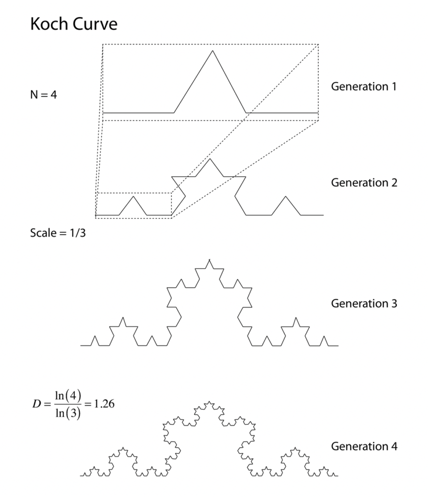
An alternative approach was proposed by Helge von Koch (1870—1924), a Swedish mathematician with an interest in number theory. He suggested in 1904 that a set of straight line segments could be joined together, and then shrunk by a scale factor to act as new segments of the original pattern [8]. The construction of the Koch curve is shown in Fig. 4. When the process is taken to its limit, it produces a curve, differentiable nowhere, which snakes through two dimensions. When connected with other identical curves into a hexagon, the curve resembles a snowflake, and the construction is known as “Koch’s Snowflake”.
The Koch curve begins in generation 1 with N0 = 4 elements. These are shrunk by a factor of b = 1/3 to become the four elements of the next generation, and so on. The number of elements varies with the observation scale according to the equation
where D is called the fractal dimension. In the example of the Koch curve, the fractal dimension is
which is a number less than its embedding dimenion DE = 2. The fractal is embedded in 2D but has a fractional dimension that is greater than it topological dimension DT = 1.
Fig. 4 Generation of a Koch curve (1904). The fractal dimension is D = ln(4)/ln(3) = 1.26. At each stage, four elements are reduced in size by a factor of 3. The “length” of the curve approaches infinity as the features get smaller and smaller. But the scaling of the length with size is determined uniquely by the fractal dimension.
Waclaw Sierpinski (1915)
Waclaw Sierpinski (1882 – 1969) was a Polish mathematician studying at the Jagellonian University in Krakow for his doctorate when he came across a theorem that every point in the plane can be defined by a single coordinate. Intrigued by such an unintuitive result, he dived deep into Cantor’s set theory after he was appointed as a faculty member at the university in Lvov. He began to construct curves that had more specific properties than the Peano or Hilbert curves, such as a curve that passes through every interior point of a unit square but that encloses an area that is only equal to 5/12 = 0.4167. Sierpinski became interested in the topological properties of such sets.
Sierpinski considered how to define a curve that was embedded in DE = 2 but that was NOT constructed as a topological dimension DT = 1 curve as the curves of Peano, Hilbert, Koch (and even his own) had been. To demonstrate this point, he described a construction that began with a topological dimension DT = 2 object, a planar triangle, from which the open set of its central inverted triangle is removed, leaving its boundary points. The process is continued iteratively to all scales [9]. The resulting point set is shown in Fig. 5 and is called the Sierpinski gasket. What is left after all the internal triangles are removed is a point set that can be made discontinuous by cutting it at a finite set of points. This is shown in Fig. 5 by the red circles. Each circle, no matter the size, cuts the set at three points, making the resulting set discontinuous. Ten years later, Karl Menger would show that this property of discontinuous cuts determined the topological dimension of the Sierpinski gasket to be DT = 1. The embedding dimension is of course DE = 2, and the fractal dimension of the Sierpinski gasket is
Fig. 5 The Sierpinski gasket. The central triangle is removed (leaving its boundary) at each scale. The pattern is self-similar with a fractal dimension DH = 1.5850. Unintuitively, it has a topological dimension DT = 1.
Felix Hausdorff (1918)
The work by Cantor, Peano, von Koch and Sierpinski had created a crisis in geometry as mathematicians struggled to rescue concepts of dimensionality. An important byproduct of that struggle was a much deeper understanding of concepts of space, especially in the hands of Felix Hausdorff.
Felix Hausdorff (1868 – 1942) was born in Breslau, Prussia, and educated in Leipzig. In his early years as a doctoral student, and as an assistant professor at Leipzig, he was a practicing mathematician by day and a philosopher and playwright by night, publishing under the pseudonym Paul Mongré. He was at the University of Bonn working on set theory when the Greek mathematician Constatin Carathéodory published a paper in 1914 that showed how to construct a p-dimensional set in a q-dimensional space [9]. Haussdorff realized that he could apply similar ideas to the Cantor set. He showed that the outer measure of the Cantor set would go discontinuously from zero to infinity as the fractional dimension increased smoothly. The critical value where the measure changed its character became known as the Hausdorff dimension [11].
For the Cantor ternary set, the Hausdorff dimension is exactly DH = ln(2)/ln(3) = 0.6309. This value for the dimension is less than the embedding dimension DE = 1 of the support (the real numbers on the interval [0, 1]), but it is also greater than DT = 0 which would hold for a countable number of points on the interval. The work by Hausdorff became well known in the mathematics community who applied the idea to a broad range of point sets like Weierstrass’s monster and the Koch curve.
It is important to keep a perspective of what Hausdorff’s work meant during which period of time. For instance, although the curves of Weierstrass, von Koch and Sierpinski were understood to present a challenge to concepts of dimension, it was only after Haussdorff that mathematicians began to think in terms of fractional dimensions and to calculate the fractional dimensions of these earlier point sets. Despite the fact that Sierpinski created one of the most iconic fractals that we use as an example every day, he was unaware at the time that he was doing so. His interest was topological—creating a curve for which any cut at any point would create disconnected subsets starting with objects (triangles) with topological dimension DT = 2. In this way, talking about the early fractal objects tends to be anachronistic, using language to describe them that had not yet been invented at that time.
This perspective is also true for the ideas of topological dimension. For instance, even Sierpinski was not fully tuned into the problems of defining topological dimension. It turns out that what he created was a curve of topological dimension DT = 1, but that would only become clear later with the work of the Austrian mathematician Karl Menger.
Karl Menger (1926)
The day that Karl Menger (1902 – 1985) was born, his father, Carl Menger (1840 – 1941) lost his job. Carl Menger was one of the founders of the famous Viennese school that established the marginalist view of economics. However, Carl was not married to Karl’s mother, which was frowned upon by polite Vienna society, so he had to relinquish his professorship. Despite his father’s reduction in status, Karl received an excellent education at a Viennese gymnasium (high school). Among of his classmates were Wolfgang Pauli (Nobel Prize for Physics in 1945) and Richard Kuhn (Nobel Prize for Chemistry in 1938). When Karl began attending the University of Vienna he studied physics, but the mathematics professor Hans Hahn opened his eyes to the fascinating work on analysis that was transforming mathematics at that time, so Karl shifted his studies to mathematical analysis, specifically concerning conceptions of “curves”.
Menger made important contributions to the history of fractal dimension as well as the history of topological dimension. In his approach to defining the intrinsic topological dimension of a point set, he described the construction of a point set embedded in three dimensions that had zero volume, an infinite surface area, and a fractal dimension between 2 and 3. The object is shown in Fig. 6 and is called a Menger “sponge” [12]. The Menger sponge is a fractal with a fractal dimension DH = ln(20)/ln(3) = 2.7268. The face of the sponge is also known as the Sierpinski carpt. The fractal dimension of the Sierpinski carpet is DH = ln(8)/ln(3) = 1.8928.
Fig. 6 Menger Sponge. Embedding dimension DE = 3. Fractal dimension DH = ln(20)/ln(3) = 2.7268. Topological dimension DT = 1: all one-dimensional metric spaces can be contained within the Menger sponge point set. Each face is a Sierpinski carpet with fractal dimension DH = ln(8)/ln(3) = 1.8928.
The striking feature of the Menger sponge is its topological dimension. Menger created a new definition of topological dimension that partially solved the crises created by Cantor when he showed that every point on the unit square can be defined by a single coordinate. This had put a one dimensional curve in one-to-one correspondence with a two-dimensional plane. Yet the topology of a 2-dimensional object is clearly different than the topology of a line. Menger found a simple definition that showed why 2D is different, topologically, than 3D, despite Cantor’s conundrum. The answer came from the idea of making cuts on a point set and seeing if the cut created disconnected subsets.
As a simple example, take a 1D line. The removal of a single point creates two disconnected sub-lines. The intersection of the cut with the line is 0-dimensional, and Menger showed that this defined the line as 1-dimensional. Similarly, a line cuts the unit square into to parts. The intersection of the cut with the plane is 1-dimensional, signifying that the dimension of the plane is 2-dimensional. In other words, a (n-1) dimensional intersection of the boundary of a small neighborhood with the point set indicates that the point set has a dimension of n. Generalizing this idea, looking at the Sierpinski gasket in Fig. 5, the boundary of a small circular region, if placed appropriately (as in the figure), intersects the Sierpinski gasket at three points of dimension zero. Hence, the topological dimension of the Sierpinski gasket is one-dimensional. Manger was likewise able to show that his sponge also had a topology that was one-dimensional, DT = 1, despite the embedding dimension of DE = 3. In fact, all 1-dimensional metric spaces can be fit inside a Menger Sponge.
Benoit Mandelbrot (1967)
Benoit Mandelbrot (1924 – 2010) was born in Warsaw and his family emigrated to Paris in 1935. He attended the Ecole Polytechnique where he studied under Gaston Julia (1893 – 1978) and Paul Levy (1886 – 1971). Both Julia and Levy made significant contributions to the field of self-similar point sets and made a lasting impression on Mandelbrot. He went to Cal Tech for a master’s degree in aeronautics and then a PhD in mathematical sciences from the University of Paris. In 1958 Mandelbrot joined the research staff of the IBM Thomas J. Watson Research Center in Yorktown Heights, New York where he worked for over 35 years on topics of information theory and economics, always with a view of properties of self-similar sets and time series.
In 1967 Mandelbrot published one of his early important papers on the self-similar properties of the coastline of Britain. He proposed that many natural features had statistical self similarity, which he applied to coastlines. He published the work as “How Long Is the Coast of Britain? Statistical Self-Similarity and Fractional Dimension” [13] in Science magazine , where he showed that the length of the coastline diverged with a Hausdorff dimension equal to D = 1.25. Working at IBM, a world leader in computers, he had ready access to their power as well as their visualization capabilities. Therefore, he was one of the first to begin exploring the graphical character of self-similar maps and point sets.
During one of his sabbaticals at Harvard University he began exploring the properties of Julia sets (named after his former teacher at the Ecole Polytechnique). The Julia set is a self-similar point set that is easily visualized in the complex plane (two dimensions). As Mandelbrot studied the convergence of divergence of infinite series defined by the Julia mapping, he discovered an infinitely nested pattern that was both beautiful and complex. This has since become known as the Mandelbrot set.
Later, in 1975, Mandelbrot coined the term fractal to describe these self-similar point sets, and he began to realize that these types of sets were ubiquitous in nature, ranging from the structure of trees and drainage basins, to the patterns of clouds and mountain landscapes. He published his highly successful and influential book The Fractal Geometry of Nature in 1982, introducing fractals to the wider public and launching a generation of hobbyists interested in computer-generated fractals. The rise of fractal geometry coincided with the rise of chaos theory that was aided by the same computing power. For instance, important geometric structures of chaos theory, known as strange attractors, have fractal geometry.
By David D. Nolte, Dec. 26, 2020
Appendix: Box Counting
When confronted by a fractal of unknown structure, one of the simplest methods to find the fractal dimension is through box counting. This method is shown in Fig. 8. The fractal set is covered by a set of boxes of size b, and the number of boxes that contain at least one point of the fractal set are counted. As the boxes are reduced in size, the number of covering boxes increases as
To be numerically accurate, this method must be iterated over several orders of magnitude. The number of boxes covering a fractal has this characteristic power law dependence, as shown in Fig. 8, and the fractal dimension is obtained as the slope.
Fig. 8 Calculation of the fractal dimension using box counting. At each generation, the size of the grid is reduced by a factor of 3. The number of boxes that contain some part of the fractal curve increases as , where b is the scale
The Physics of Life, the Universe and Everything:
Read more about the history of modern dynamics and fractals, in Galileo Unbound from Oxford University Press
[1] Hardy, G. (1916). “Weierstrass’s non-differentiable function.” Transactions of the American Mathematical Society 17: 301-325.
[2] Weierstrass, K. (1872). “Uber continuirliche Functionen eines reellen Arguments, die fur keinen Werth des letzteren einen bestimmten Differentialquotienten besitzen.” Communication ri I’Academie Royale des Sciences II: 71-74.
[3] Besicovitch, A. S. and H. D. Ursell (1937). “Sets of fractional dimensions: On dimensional numbers of some continuous curves.” J. London Math. Soc. 1(1): 18-25.
[4] Shen, W. (2018). “Hausdorff dimension of the graphs of the classical Weierstrass functions.” Mathematische Zeitschrift. 289(1–2): 223–266.
[5] Cantor, G. (1883). Grundlagen einer allgemeinen Mannigfaltigkeitslehre. Leipzig, B. G. Teubner.
[6] Peano, G. (1890). “Sur une courbe qui remplit toute une aire plane.” Mathematische Annalen 36: 157-160.
[7] Peano, G. (1888). Calcolo geometrico secundo l’Ausdehnungslehre di H. Grassmann e precedutto dalle operazioni della logica deduttiva. Turin, Fratelli Bocca Editori.
[8] Von Koch, H. (1904). “Sur.une courbe continue sans tangente obtenue par une construction geometrique elementaire.” Arkiv for Mathematik, Astronomi och Fysich 1: 681-704.
[9] Sierpinski, W. (1915). “Sur une courbe dont tout point est un point de ramification.” Comptes Rendus Hebdomadaires des Seances de l’Academie des Sciences de Paris 160: 302-305.
[10] Carathéodory, C. (1914). “Über das lineare Mass von Punktmengen – eine Verallgemeinerung des Längenbegriffs.” Gött. Nachr. IV: 404–406.
[11] Hausdorff, F. (1919). “Dimension und ausseres Mass.” Mathematische Anna/en 79: 157-179.
[12] Menger, Karl (1926), “Allgemeine Räume und Cartesische Räume. I.”, Communications to the Amsterdam Academy of Sciences. English translation reprinted in Edgar, Gerald A., ed. (2004), Classics on fractals, Studies in Nonlinearity, Westview Press. Advanced Book Program, Boulder, CO
[13] B Mandelbrot, How Long Is the Coast of Britain? Statistical Self-Similarity and Fractional Dimension. Science, 156 3775 (May 5, 1967): 636-638.