Snorkeling above a shallow reef on a clear sunny day transports you to an otherworldly galaxy of spectacular deep colors and light reverberating off of the rippled surface.  Playing across the underwater floor of the reef is a fabulous light show of bright filaments entwining and fluttering, creating random mesh networks of light and dark.  These same patterns appear on the bottom of swimming pools in summer and in deep fountains in parks.

Johann Bernoulli had a stormy career and a problematic personality–but he was brilliant even among the bountiful Bernoulli clan. Using methods of tangents, he found the analytic solution of the caustic of the circle.

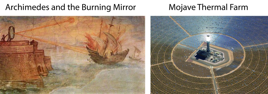
Something similar happens when a bare overhead light reflects from the sides of a circular glass of water.  The pattern no longer moves, but a dazzling filament splays across the bottom of the glass with a sharp bright cusp at the center. These bright filaments of light have an age old name — Caustics — meaning burning as in burning with light. The study of caustics goes back to Archimedes of Syracuse and his apocryphal burning mirrors that are supposed to have torched the invading triremes of the Roman navy in 212 BC.

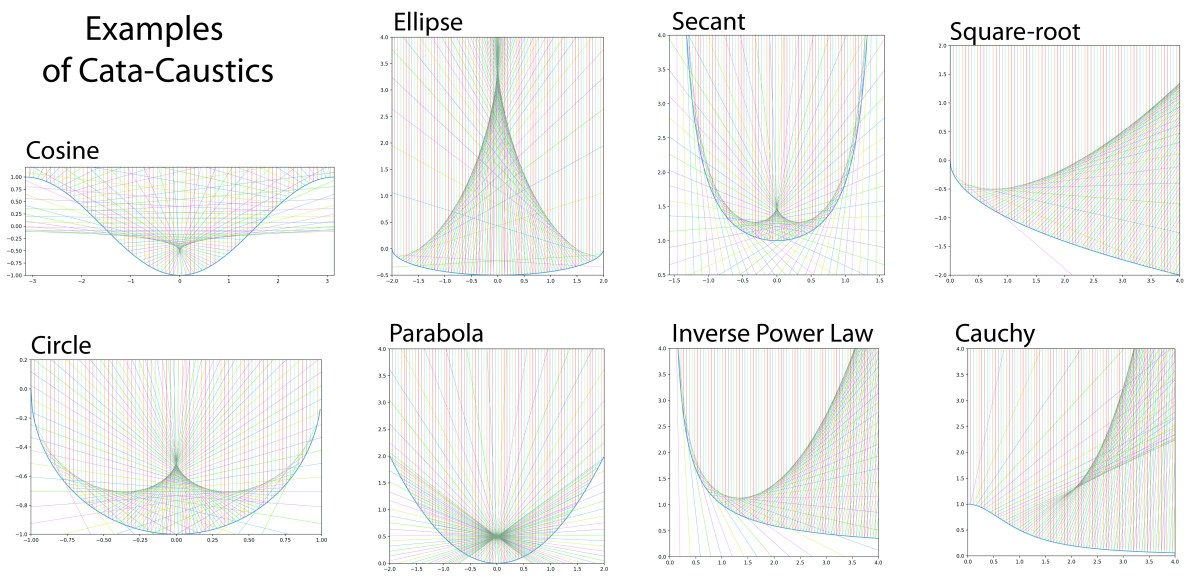
Caustics in optics are concentrations of light rays that form bright filaments, often with cusp singularities. Mathematically, they are envelope curves that are tangent to a set of lines. Cata-caustics are caustics caused by light reflecting from curved surfaces. Dia-caustics are caustics caused by light refracting from transparent curved materials.

From Leonardo to Huygens

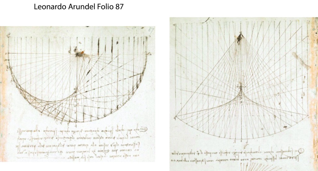
Even after Archimedes, burning mirrors remained an interest for a broad range of scientists, artists and engineers. Leonardo Da Vinci took an interest around 1503 – 1506 when he drew reflected caustics from a circular mirror in his many notebooks.

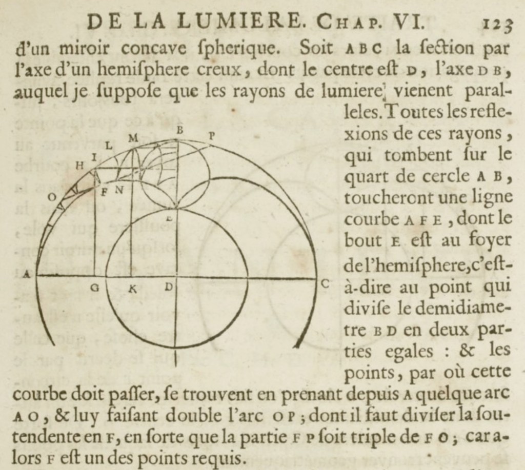
Almost two centuries later, Christian Huygens constructed the caustic of a circle in his Treatise on light : in which are explained the causes of that which occurs in reflection, & in refraction and particularly in the strange refraction of Iceland crystal. This is the famous treatise in which he explained his principle for light propagation as wavefronts. He was able to construct the caustic geometrically, but did not arrive at a functional form. He mentions that it has a cusp like a cycloid, but without being a cycloid. He first presented this work at the Paris Academy in 1678 where the news of his lecture went as far as Italy where a young German mathematician was traveling.

The Cata-caustics of Tschirnhaus and Bernoulli

In the decades after Newton and Leibniz invented the calculus, a small cadre of mathematicians strove to apply the new method to understand aspects of the physical world. At at a time when Newton had left the calculus behind to follow more arcane pursuits, Lebniz, Jakob and Johann Bernoulli, Guillaume de l’Hôpital, Émilie du Chatelet and Walter von Tschirnhaus were pushing notation reform (mainly following Leibniz) to make the calculus easier to learn and use, as well as finding new applications of which there were many.

Ehrenfried Walter von Tschirnhaus (1651 – 1708) was a German mathematician and physician and a lifelong friend of Leibniz, who he met in Paris in 1675. He was one of only five mathematicians to provide a solution to Johann Bernoulli’s brachistochrone problem. One of the recurring interests of von Tschirnhaus, that he revisited throughout his carrier, was in burning glasses and mirrors. A burning glass is a high-quality magnifying lens that brings the focus of the sun to a fine point to burn or anneal various items. Burning glasses were used to heat small items for manufacture or for experimentation. For instance, Priestly and Lavoisier routinely used burning glasses in their chemistry experiments. Low optical aberrations were required for the lenses to bring the light to the finest possible focus, so the study of optical focusing was an important topic both academically and practically. Tshirnhaus had his own laboratory to build and test burning mirrors, and he became aware of the cata-caustic patterns of light reflected from a circular mirror or glass surface. Given his parallel interest in the developing calculus methods, he published a paper in Acta Eruditorum in 1682 that constructed the envelope function created by the cata-caustics of a circle. However, Tschirnhaus did not produce the analytic function–that was provided by Johann Bernoulli ten years later in 1692.

Johann Bernoulli had a stormy career and a problematic personality–but he was brilliant even among the Bountiful Bernoulli clan. Using methods of tangents, he found the analytic solution of the caustic of the circle. He did this by stating the general equation for all reflected rays and then finding when their y values are independent of changing angle … in other words using the principle of stationarity which would later become a potent tool in the hands of Lagrange as he developed Lagrangian physics.

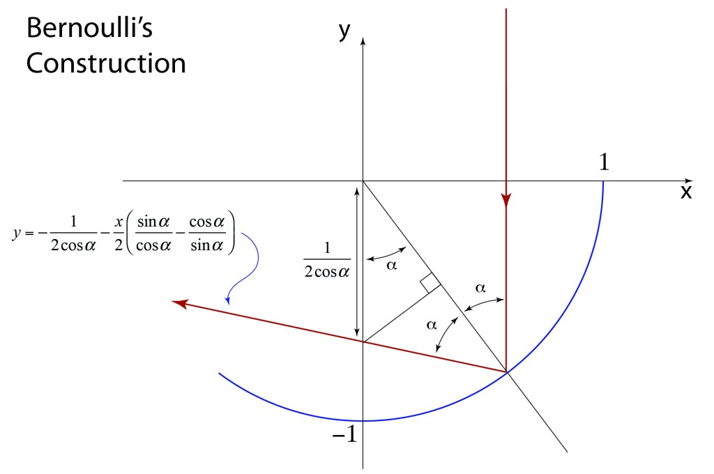
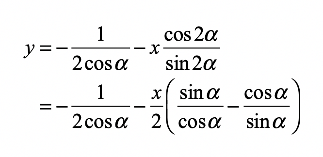
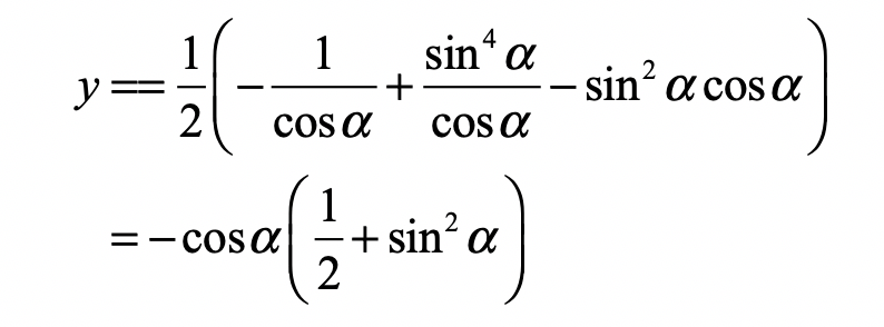
The equation for the reflected ray, expressing y as a function of x for a given angle α in Fig. 5, is

The condition of the caustic envelope requires the change in y with respect to the angle α to vanish while treating x as a constant. This is a partial derivative, and Johann Bernoulli is giving an early use of this method in 1692 to ensure the stationarity of y with respect to the changing angle. The partial derivative is

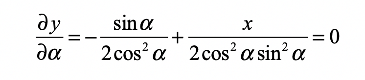
This is solved to give

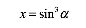
Plugging this into the equation at the top equation above yields

These last two expressions for x and y in terms of the angle α are a parametric representation of the caustic. Combining them gives the solution to the caustic of the circle

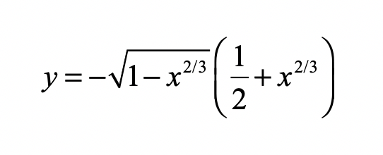
The square root provides the characteristic cusp at the center of the caustic.

Python Code: raycaustic.py

There are lots of options here. Try them all … then add your own!

#!/usr/bin/env python3
# -*- coding: utf-8 -*-
"""
Created on Tue Feb 16 16:44:42 2021

raycaustic.py

@author: nolte

D. D. Nolte, Optical Interferometry for Biology and Medicine (Springer,2011)
"""

import numpy as np
from matplotlib import pyplot as plt

plt.close('all')

# model_case 1 = cosine
# model_case 2 = circle
# model_case 3 = square root
# model_case 4 = inverse power law
# model_case 5 = ellipse
# model_case 6 = secant
# model_case 7 = parabola
# model_case 8 = Cauchy

model_case = int(input('Input Model Case (1-7)'))
if model_case == 1:
    model_title = 'cosine'
    xleft = -np.pi
    xright = np.pi
    ybottom = -1
    ytop = 1.2

elif model_case == 2:
    model_title = 'circle'
    xleft = -1
    xright = 1
    ybottom = -1
    ytop = .2

elif model_case == 3:
    model_title = 'square-root'
    xleft = 0
    xright = 4
    ybottom = -2
    ytop = 2

elif model_case == 4:
    model_title = 'Inverse Power Law'
    xleft = 1e-6
    xright = 4
    ybottom = 0
    ytop = 4
    
elif model_case == 5:
    model_title = 'ellipse'
    a = 0.5
    b = 2
    xleft = -b
    xright = b
    ybottom = -a
    ytop = 0.5*b**2/a
    
elif model_case == 6:
    model_title = 'secant'
    xleft = -np.pi/2
    xright = np.pi/2
    ybottom = 0.5
    ytop = 4
    
elif model_case == 7:
    model_title = 'Parabola'
    xleft = -2
    xright = 2
    ybottom = 0
    ytop = 4

elif model_case == 8:
    model_title = 'Cauchy'
    xleft = 0
    xright = 4
    ybottom = 0
    ytop = 4
    
def feval(x):

    if model_case == 1:
        y = -np.cos(x)

    elif model_case == 2:
        y = -np.sqrt(1-x**2)

    elif model_case == 3:
        y = -np.sqrt(x)
        
    elif model_case == 4:
        y = x**(-0.75)
        
    elif model_case == 5:
        y = -a*np.sqrt(1-x**2/b**2)

    elif model_case == 6:
        y = 1.0/np.cos(x)

    elif model_case == 7:
        y = 0.5*x**2  
        
    elif model_case == 8:
        y = 1/(1 + x**2)

    return y

xx = np.arange(xleft,xright,0.01)
yy = feval(xx)

lines = plt.plot(xx,yy)
plt.xlim(xleft, xright)
plt.ylim(ybottom, ytop)

delx = 0.001
N = 75

for i in range(N+1):
    
    x = xleft + (xright-xleft)*(i-1)/N
    
    val = feval(x)
    valp = feval(x+delx/2)
    valm = feval(x-delx/2)
    deriv = (valp-valm)/delx
    
    phi = np.arctan(deriv)
    slope =  np.tan(np.pi/2 + 2*phi)

    if np.abs(deriv) < 1:
        xf = (ytop-val+slope*x)/slope;
        yf = ytop;
    else:
        xf = (ybottom-val+slope*x)/slope;
        yf = ybottom;
    plt.plot([x, x],[ytop, val],linewidth = 0.5)       
    plt.plot([x, xf],[val, yf],linewidth = 0.5)
    plt.gca().set_aspect('equal', adjustable='box')       
    plt.show()
    

The Dia-caustics of Swimming Pools

A caustic is understood mathematically as the envelope function of multiple rays that converge in the Fourier domain (angular deflection measured at far distances).  These are points of mathematical stationarity, in which the ray density is invariant to first order in deviations in the refracting surface.  The rays themselves are the trajectories of the Eikonal Equation as rays of light thread their way through complicated optical systems.

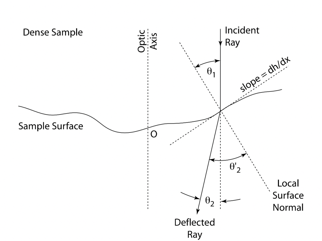
The basic geometry is shown in Fig 7 for a ray incident on a nonplanar surface emerging into a less-dense medium.  From Snell’s law we have the relation for light entering a dense medium like light into water

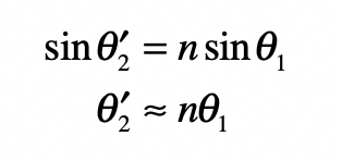
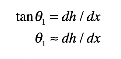
where n is the relative index (ratio), and the small-angle approximation has been made.  The incident angle θ₁ is simply related to the slope of the interface dh/dx as

where the small-angle approximation is used again.  The angular deflection relative to the optic axis is then

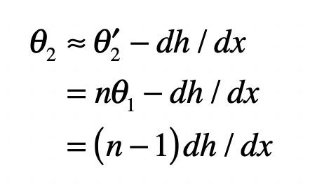
which is equal to the optical path difference through the sample.

In two dimensions, the optical path difference can be replaced with a general potential

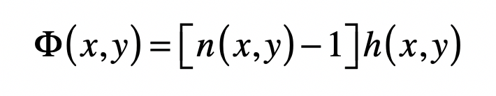
and the two orthogonal angular deflections (measured in the far field on a Fourier plane) are

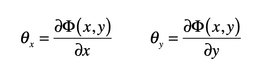
These angles describe the deflection of the rays across the sample surface. They are also the right-hand side of the Eikonal Equation, the equation governing ray trajectories through optical systems.

Caustics are lines of stationarity, meaning that the density of rays is independent of first-order changes in the refracting sample.  The condition of stationarity is defined by the Jacobian of the transformation from (x,y) to (θ_x, θ_y) with

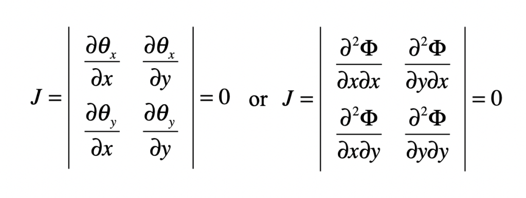
where the second expression is the Hessian determinant of the refractive power of the uneven surface. When this condition is satisfied, the envelope function bounding groups of collected rays is stationary to perturbations in the inhomogeneous sample.

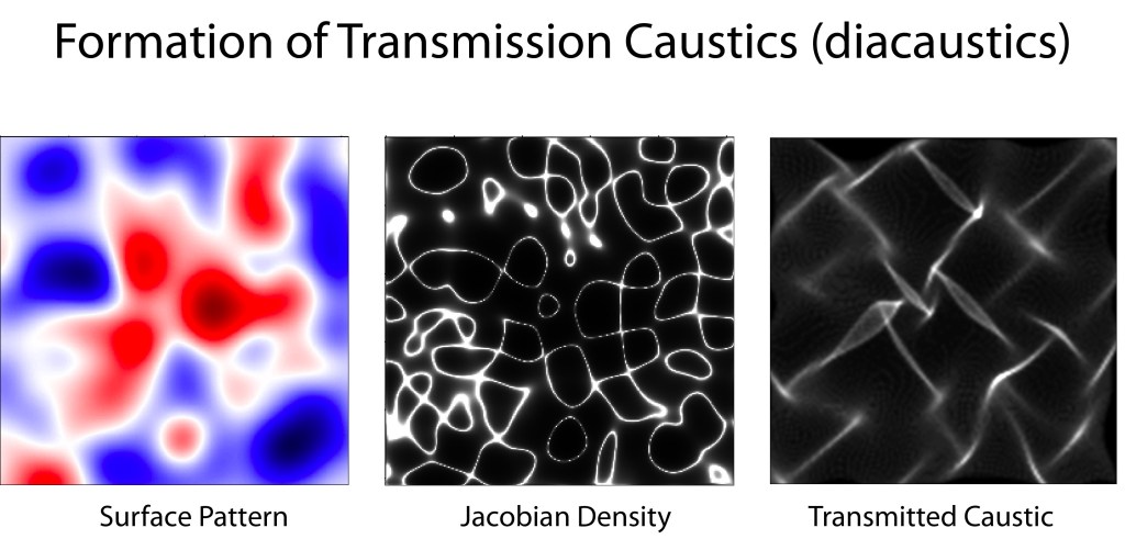
An example of diacaustic formation from a random surface is shown in Fig. 8 generated by the Python program caustic.py. The Jacobian density (center) outlines regions in which the ray density is independent of small changes in the surface. They are positions of the zeros of the Hessian determinant, the regions of zero curvature of the surface or potential function. These high-intensity regions spread out and are intercepted at some distance by a suface, like the bottom of a swimming pool, where the concentrated rays create bright filaments. As the wavelets on the surface of the swimming pool move, the caustic filaments on the bottom of the swimming pool dance about.

Optical caustics also occur in the gravitational lensing of distant quasars by galaxy clusters in the formation of Einstein rings and arcs seen by deep field telescopes, as described in my following blog post.

Python Code: caustic.py

This Python code was used to generate the caustic patterns in Fig. 8. You can change the surface roughness by changing the divisors on the last two arguments on Line 58. The distance to the bottom of the swimming pool can be changed by changing the parameter d on Line 84.

#!/usr/bin/env python3
# -*- coding: utf-8 -*-
"""
Created on Tue Feb 16 19:50:54 2021

caustic.py

@author: nolte

D. D. Nolte, Optical Interferometry for Biology and Medicine (Springer,2011)
"""

import numpy as np
from matplotlib import pyplot as plt
from numpy import random as rnd
from scipy import signal as signal

plt.close('all')

N = 256

def gauss2(sy,sx,wy,wx):
    
    x = np.arange(-sx/2,sy/2,1)
    y = np.arange(-sy/2,sy/2,1)
    y = y[..., None]
    
    ex = np.ones(shape=(sy,1))
    x2 = np.kron(ex,x**2/(2*wx**2));
    
    ey = np.ones(shape=(1,sx));
    y2 = np.kron(y**2/(2*wy**2),ey);

    rad2 = (x2+y2);

    A = np.exp(-rad2);

    return A

def speckle2(sy,sx,wy,wx):

    Btemp = 2*np.pi*rnd.rand(sy,sx);
    B = np.exp(complex(0,1)*Btemp);

    C = gauss2(sy,sx,wy,wx);

    Atemp = signal.convolve2d(B,C,'same');

    Intens = np.mean(np.mean(np.abs(Atemp)**2));

    D = np.real(Atemp/np.sqrt(Intens));

    Dphs = np.arctan2(np.imag(D),np.real(D));

    return D, Dphs


Sp, Sphs = speckle2(N,N,N/16,N/16)

plt.figure(2)
plt.matshow(Sp,2,cmap=plt.cm.get_cmap('seismic'))  # hsv, seismic, bwr
plt.show()

fx, fy = np.gradient(Sp);

fxx,fxy = np.gradient(fx);
fyx,fyy = np.gradient(fy);

J = fxx*fyy - fxy*fyx;

D = np.abs(1/J)

plt.figure(3)
plt.matshow(D,3,cmap=plt.cm.get_cmap('gray'))  # hsv, seismic, bwr
plt.clim(0,0.5e7)
plt.show()

eps = 1e-7
cnt = 0
E = np.zeros(shape=(N,N))
for yloop in range(0,N-1):
    for xloop in range(0,N-1):
        
        d = N/2
        
        indx = int(N/2 + (d*(fx[yloop,xloop])+(xloop-N/2)/2))
        indy = int(N/2 + (d*(fy[yloop,xloop])+(yloop-N/2)/2))
        
        if ((indx > 0) and (indx < N)) and ((indy > 0) and (indy < N)):
            E[indy,indx] = E[indy,indx] + 1

plt.figure(4)
plt.imshow(E,interpolation='bicubic',cmap=plt.cm.get_cmap('gray'))
plt.clim(0,30)
plt.xlim(N/4, 3*N/4)
plt.ylim(N/4,3*N/4)

By David D. Nolte, Feb. 28, 2021

External Link: Youtube Video

Read more from Oxford University Press: Interference (2023)

The stories of the scientists and engineers who tamed light and used it to probe the universe.

Available at Oxford U Press

Available at Amazon.

Available at Barnes & Nobles

References

[1] D. D. Nolte, “Speckle and Spatial Coherence,” Chapter 3 in Optical Interferometry for Biology and Medicine (Springer, 2012), pp. 95-121.

[2] E. Hairer and G. Wanner, Analysis by its history. (Springer, 1996)

[3] C. Huygens (1690), Treatise on light : in which are explained the causes of that which occurs in reflection, & in refraction and particularly in the strange refraction of Iceland crystal. Ed. S. P. Thompson, (University of Chicago Press, 1950).