Einstein’s theory of gravity came from a simple happy thought that occurred to him as he imagined an unfortunate worker falling from a roof, losing hold of his hammer, only to find both the hammer and himself floating motionless relative to each other as if gravity had ceased to exist. With this one thought, Einstein realized that the falling (i.e. accelerating) reference frame was in fact an inertial frame, and hence all the tricks that he had learned and invented to deal with inertial relativistic frames could apply just as well to accelerating frames in gravitational fields.
Gravitational lensing (and microlensing) have become a major tool of discovery in astrophysics applied to the study of quasars, dark matter and even the search for exoplanets.
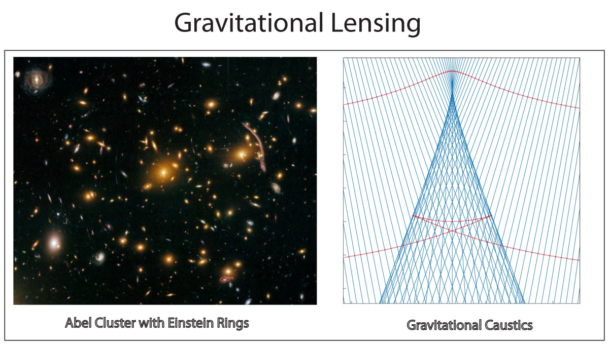
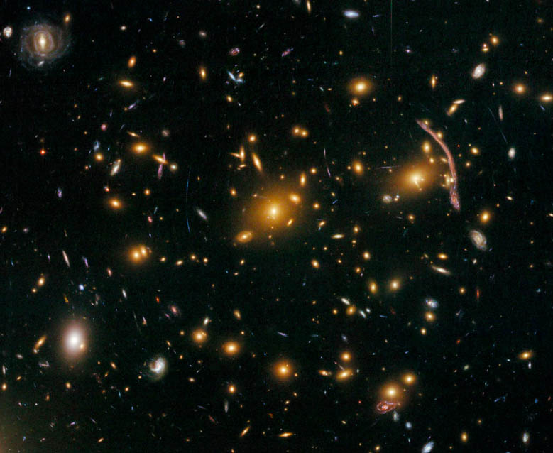
Armed with this new perspective, one of the earliest discoveries that Einstein made was that gravity must bend light paths. This phenomenon is fundamentally post-Newtonian, because there can be no possible force of gravity on a massless photon—yet Einstein’s argument for why gravity should bend light is so obvious that it is manifestly true, as demonstrated by Arthur Eddington during the solar eclipse of 1919, launching Einstein to world-wide fame. It is also demonstrated by the beautiful gravitational lensing phenomenon of Einstein arcs. Einstein arcs are the distorted images of bright distant light sources in the universe caused by an intervening massive object, like a galaxy or galaxy cluster, that bends the light rays. A number of these arcs are seen in images of the Abel cluster of galaxies in Fig. 1.
Gravitational lensing (and microlensing) have become a major tool of discovery in astrophysics applied to the study of quasars, dark matter and even the search for exoplanets. However, as soon as Einstein conceived of gravitational lensing, in 1912, he abandoned the idea as too small and too unlikely to ever be useful, much like he abandoned the idea of gravitational waves in 1915 as similarly being too small ever to detect. It was only at the persistence of an amateur Czech scientist twenty years later that Einstein reluctantly agreed to publish his calculations on gravitational lensing.
The History of Gravitational Lensing
In 1912, only a few years after his “happy thought”, and fully three years before he published his definitive work on General Relativity, Einstein derived how light would be affected by a massive object, causing light from a distant source to be deflected like a lens. The historian of physics, Jürgen Renn discovered these derivations in Einstein’s notebooks while at the Max Planck Institute for the History of Science in Berlin in 1996 [1]. However, Einstein also calculated the magnitude of the effect and dismissed it as too small, and so he never published it.
Years later, in 1936, Einstein received a visit from a Czech electrical engineer Rudi Mandl, an amateur scientist who had actually obtained a small stipend from the Czech government to visit Einstein at the Institute for Advanced Study at Princeton. Mandl had conceived of the possibility of gravitational lensing and wished to bring it to Einstein’s attention, thinking that the master would certainly know what to do with the idea. Einstein was obliging, redoing his calculations of 1912 and obtaining once again the results that made him believe that the effect would be too small to be seen. However, Mandl was persistent and pressed Einstein to publish the results, which he did [2]. In his submission letter to the editor of Science, Einstein stated “Let me also thank you for your cooperation with the little publication, which Mister Mandl squeezed out of me. It is of little value, but it makes the poor guy happy”. Einstein’s pessimism was based on his thinking that isolated stars would be the only source of the gravitational lens (he did not “believe” in black holes), but in 1937 Fritz Zwicky at Cal Tech (a gadfly genius) suggested that the newly discovered phenomenon of “galaxy clusters” might provide the massive gravity that would be required to produce the effect. Although, to be visible, a distant source would need to be extremely bright.
Potential sources were discovered in the 1960’s using radio telescopes that discovered quasi-stellar objects (known as quasars) that are extremely bright and extremely far away. Quasars also appear in the visible range, and in 1979 a twin quasar was discovered by astronomers using the telescope at the Kitt Peak Obversvatory in Arizona–two quasars very close together that shared identical spectral fingerprints. The astronomers realized that it could be a twin image of a single quasar caused by gravitational lensing, which they published as a likely explanation. Although the finding was originally controversial, the twin-image was later confirmed, and many additional examples of gravitational lensing have since been discovered.
The Optics of Gravity and Light
Gravitational lenses are terrible optical instruments. A good imaging lens has two chief properties: 1) It produces increasing delay on a wavefront as the radial distance from the optic axis decreases; and 2) it deflects rays with increasing deflection angle as the radial distance of a ray increases away from the optic axis (the center of the lens). Both properties are part of the same effect: the conversion, by a lens, of an incident plane wave into a converging spherical wave. A third property of a good lens ensures minimal aberrations of the converging wave: a quadratic dependence of wavefront delay on radial distance from the optic axis. For instance, a parabolic lens produces a diffraction-limited focal spot.
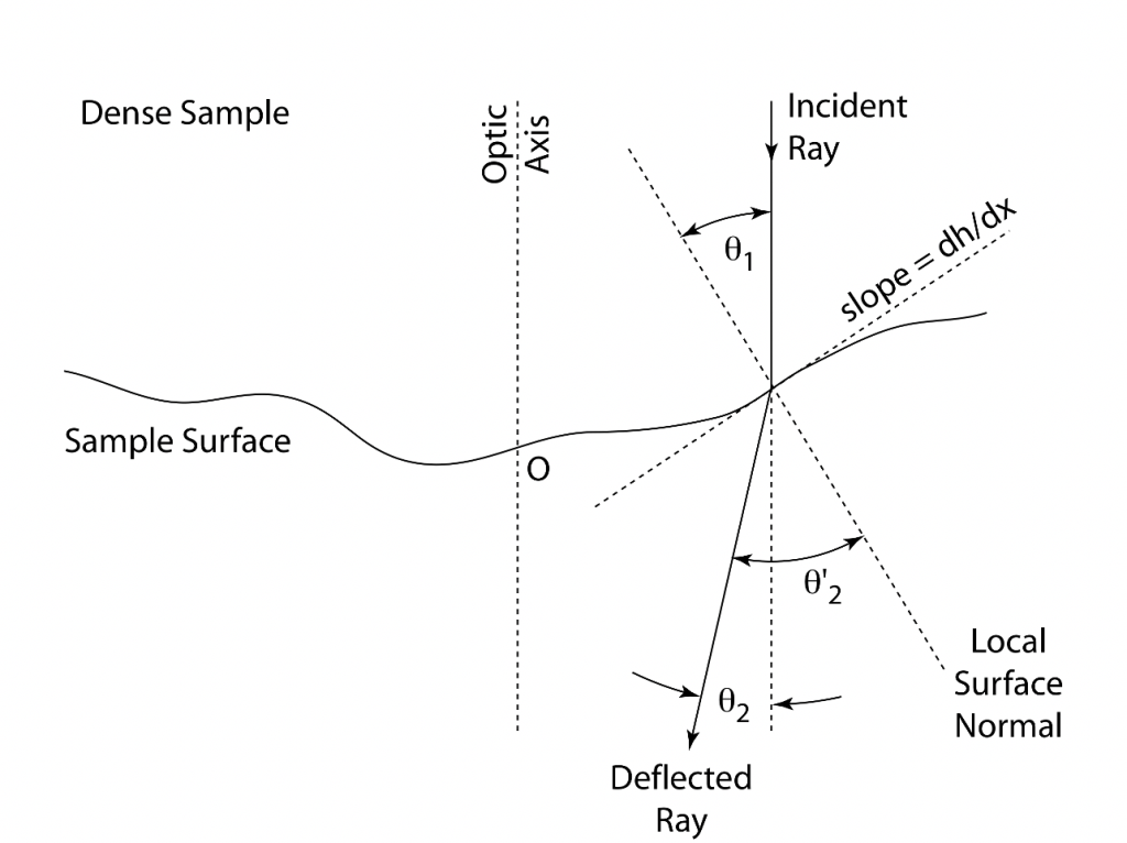
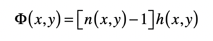
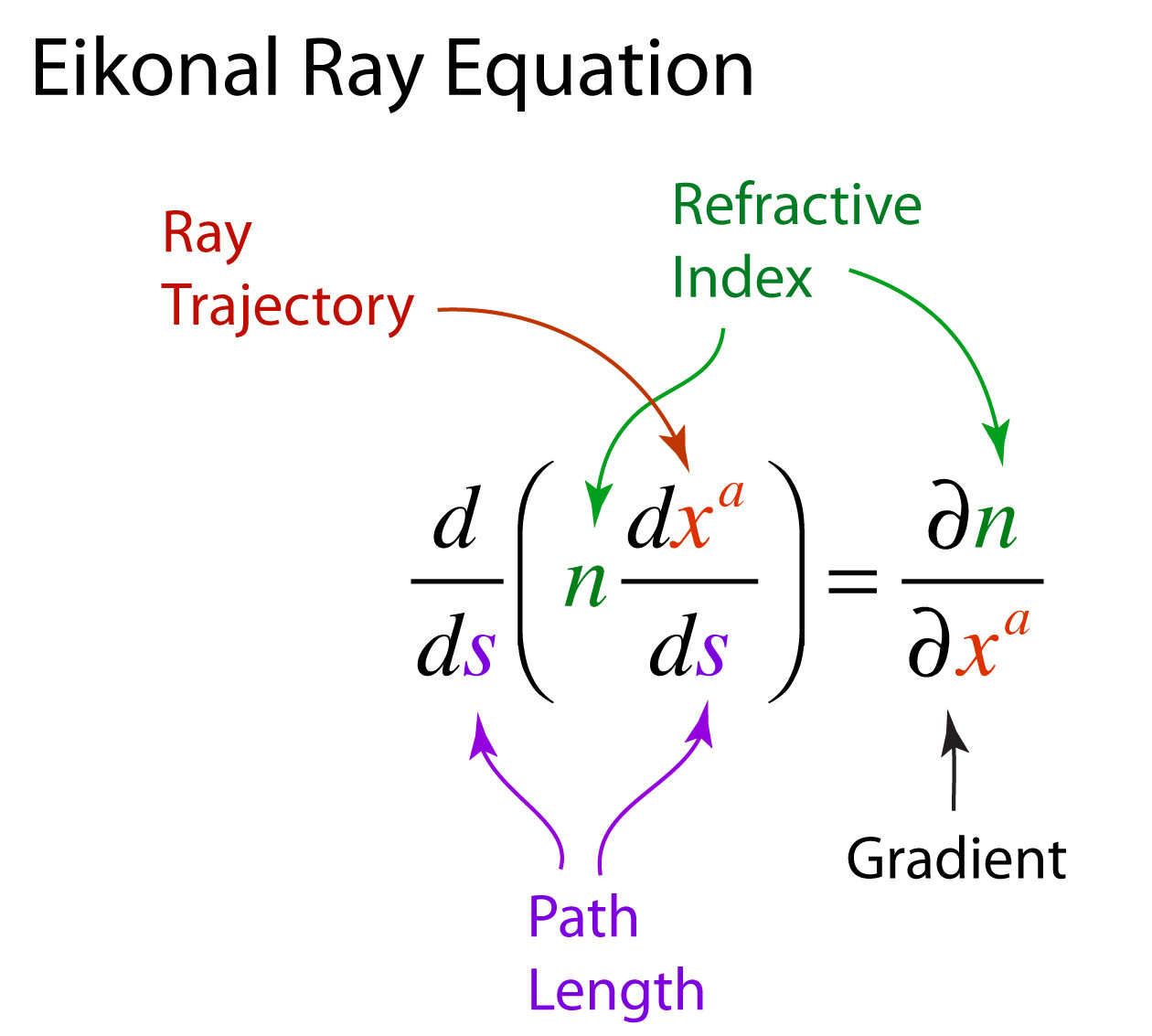
Now consider the optical effects of gravity around a black hole. One of Einstein’s chief discoveries during his early investigations into the effects of gravity on light is the analogy of warped space-time as having an effective refractive index. Light propagates through space affected by gravity as if there were a refractive index associated with the gravitational potential. In a previous blog on the optics of gravity, I showed the simple derivation of the refractive effects of gravity on light based on the Schwarschild metric applied to a null geodesic of a light ray. The effective refractive index near a black hole is
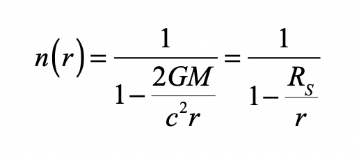
This effective refractive index diverges at the Schwarzschild radius of the black hole. It produces the maximum delay, not on the optic axis as for a good lens, but at the finite distance RS. Furthermore, the maximum deflection also occurs at RS, and the deflection decreases with increasing radial distance. Both of these properties of gravitational lensing are opposite to the properties of a good lens. For this reason, the phrase “gravitational lensing” is a bit of a misnomer. Gravitating bodies certainly deflect light rays, but the resulting optical behavior is far from that of an imaging lens.
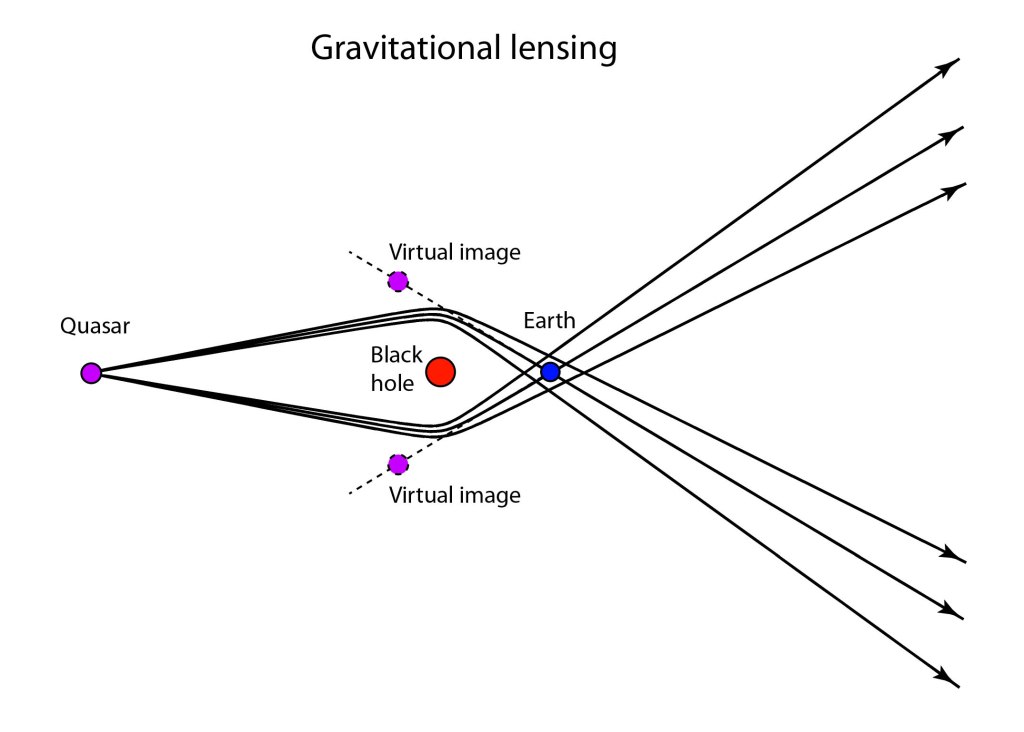
The path of a ray from a distant quasar, through the thin gravitational lens of a galaxy, and intersecting the location of the Earth, is shown in Fig. 2. The location of the quasar is a distance R from the “optic axis”. The un-deflected angular position is θ0, and with the intervening galaxy the image appears at the angular position θ. The angular magnification is therefore M = θ/θ0.
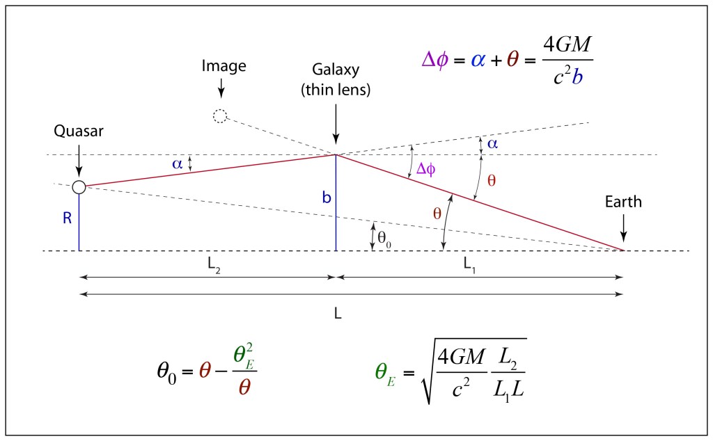
The deflection angles are related through
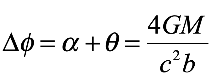
where b is the “impact parameter”
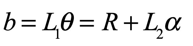
These two equations are solved to give to an expression that relates the unmagnified angle θ0 to the magnified angle θ as
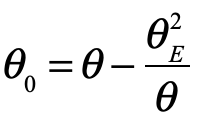
where
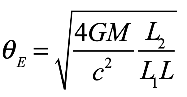
is the angular size of the Einstein ring when the source is on the optic axis. The quadratic equation has two solutions that gives two images of the distant quasar. This is the origin of the “double image” that led to the first discovery of gravitational lensing in 1979.
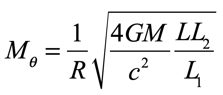
When the distant quasar is on the optic axis, then θ0 = 0 and the deflection of the rays produces, not a double image, but an Einstein ring with an angular size of θE. For typical lensing objects, the angular size of Einstein rings are typically in the range of tens of microradians. The angular magnification for decreasing distance R diverges as
But this divergence is more a statement of the bad lens behavior than of actual image size. Because the gravitational lens is inverted (with greater deflection closer to the optic axis) compared to an ideal thin lens, it produces a virtual image ring that is closer than the original object, as in Fig. 3.
The location of the virtual image behind the gravitational lens (when the quasar is on the optic axis) is obtained from
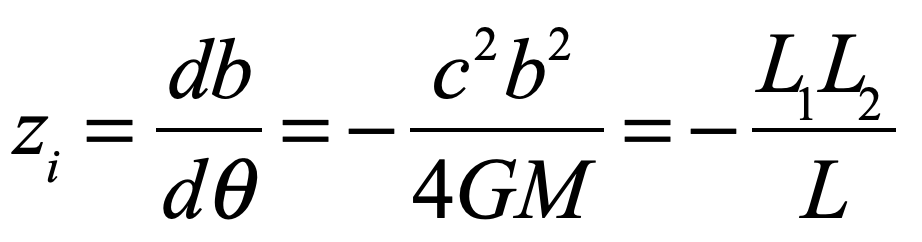
If the quasar is much further from the lens than the Earth, then the image location is zi = -L1, or behind the lens by the same distance from the Earth to the lens. The longitudinal magnification is then
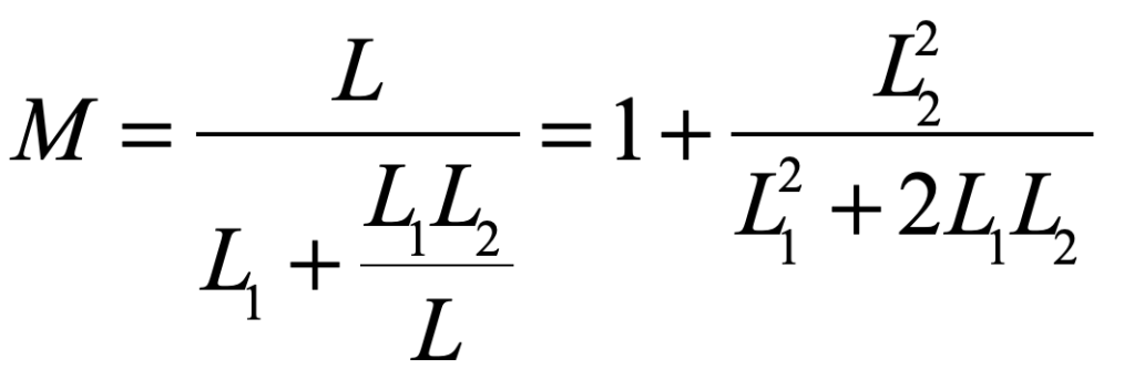
Note that while the transverse (angular) magnification diverges as the object approaches the optic axis, the longitudinal magnification remains finite but always greater than unity.
The Caustic Curves of Einstein Rings
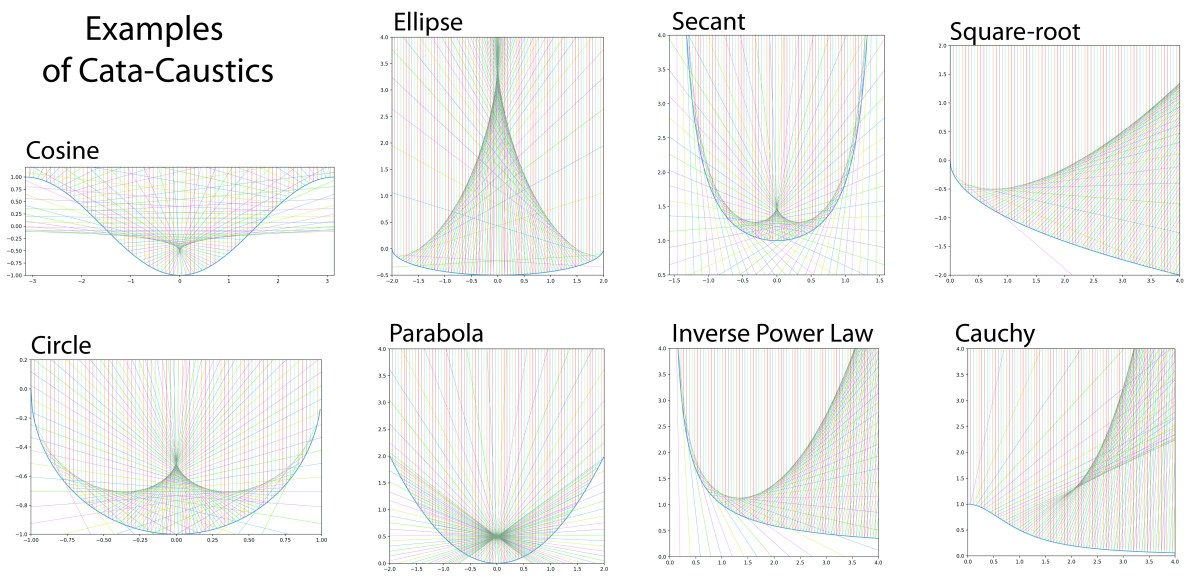
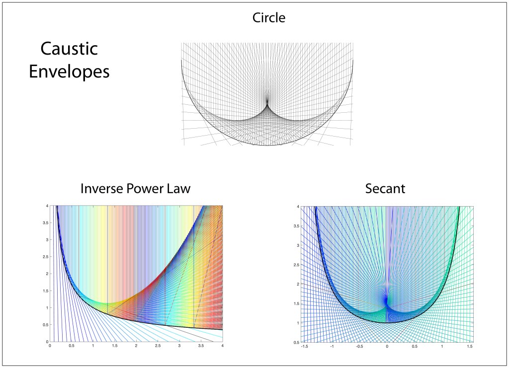
Because gravitational lenses have such severe aberration relative to an ideal lens, and because the angles are so small, an alternate approach to understanding the optics of gravity is through the theory of light caustics. In my previous blog on the optics of caustics, I described how sets of deflected rays of light become enclosed in envelopes that produce regions of high and low intensity. These envelopes are called caustics. Gravitational light deflection also causes caustics.
In addition to envelopes, it is also possible to trace the time delays caused by gravity on wavefronts. In the regions of the caustic envelopes, these wavefronts can fold back onto themselves so that different parts of the image arrive at different times coming from different directions.
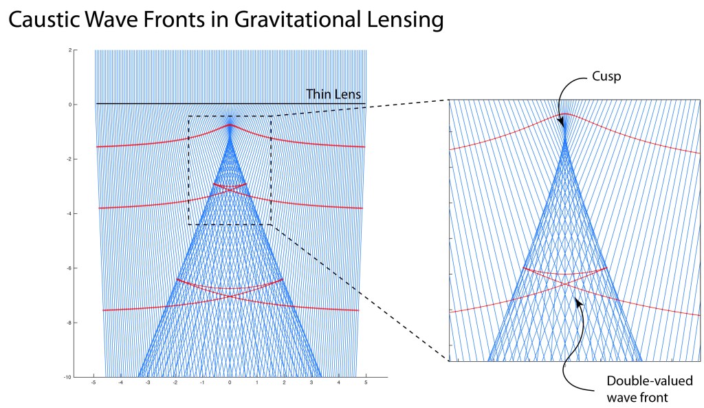
An example of gravitational caustics is shown in Fig. 4. Rays are incident vertically on a gravitational thin lens which deflects the rays so that they overlap in the region below the lens. The red curves are selected wavefronts at three successively later times. The gravitational potential causes a time delay on the propgating front, with greater delays in regions of stronger gravitational potential. The envelope function that is tangent to the rays is called the caustic, here shown as the dense blue mesh. In this case there is a cusp in the caustic near z = -1 below the lens. The wavefronts become multiple-valued past the cusp
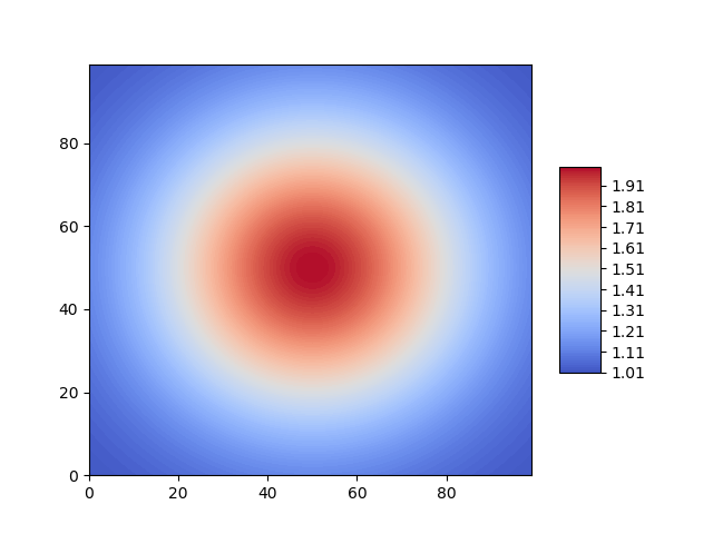
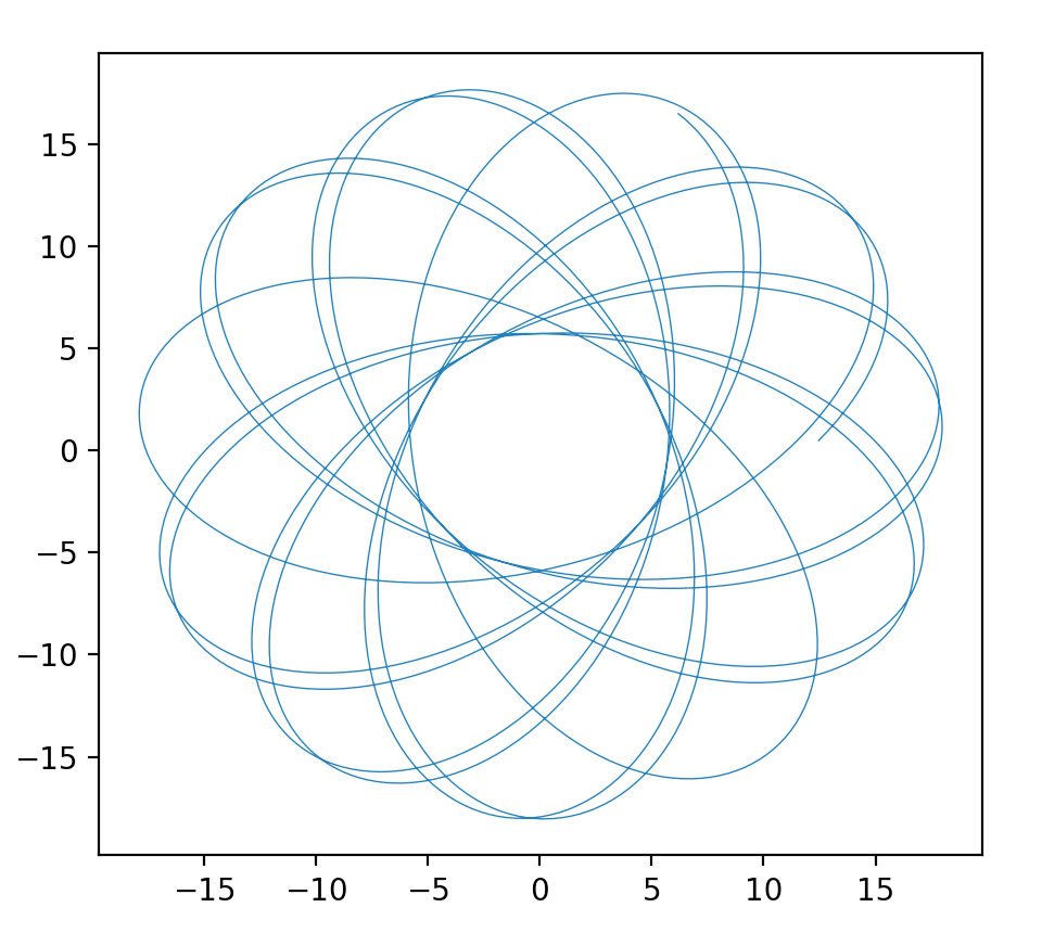
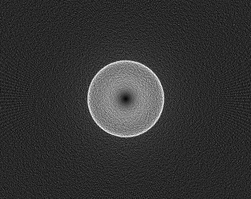
The intensity of the distant object past the lens is concentrated near the caustic envelope. The intensity of the caustic at z = -6 is shown in Fig. 5. The ring structure is the cross-sectional spatial intensity at the fixed observation plane, but a transform to the an angular image is one-to-one, so the caustic intensity distribution is also similar to the view of the Einstein ring from a position at z = -6 on the optic axis.
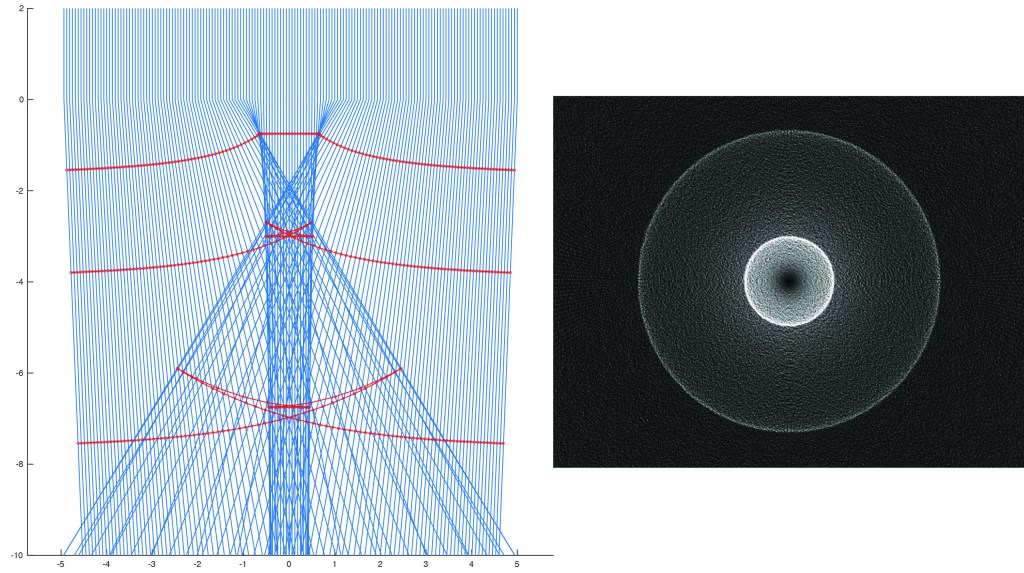
The gravitational potential is a function of the mass distribution in the gravitational lens. A different distribution with a flatter distribution of mass near the optic axis is shown in Fig. 6. There are multiple caustics in this case with multi-valued wavefronts. Because caustics are sensitive to mass distribution in the gravitational lens, astronomical observations of gravitational caustics can be used to back out the mass distribution, including dark matter or even distant exoplanets.
By David D. Nolte, April 5, 2021
Python Code gravfront.py
(Python code on GitHub.)
#!/usr/bin/env python3
# -*- coding: utf-8 -*-
"""
Created on Tue Mar 30 19:47:31 2021
gravfront.py
@author: David Nolte
Introduction to Modern Dynamics, 2nd edition (Oxford University Press, 2019)
Gravitational Lensing
"""
import numpy as np
from matplotlib import pyplot as plt
plt.close('all')
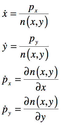
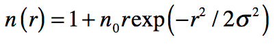
def refindex(x):
n = n0/(1 + abs(x)**expon)**(1/expon);
return n
delt = 0.001
Ly = 10
Lx = 5
n0 = 1
expon = 2 # adjust this from 1 to 10
delx = 0.01
rng = np.int(Lx/delx)
x = delx*np.linspace(-rng,rng)
n = refindex(x)
dndx = np.diff(n)/np.diff(x)
plt.figure(1)
lines = plt.plot(x,n)
plt.figure(2)
lines2 = plt.plot(dndx)
plt.figure(3)
plt.xlim(-Lx, Lx)
plt.ylim(-Ly, 2)
Nloop = 160;
xd = np.zeros((Nloop,3))
yd = np.zeros((Nloop,3))
for loop in range(0,Nloop):
xp = -Lx + 2*Lx*(loop/Nloop)
plt.plot([xp, xp],[2, 0],'b',linewidth = 0.25)
thet = (refindex(xp+delt) - refindex(xp-delt))/(2*delt)
xb = xp + np.tan(thet)*Ly
plt.plot([xp, xb],[0, -Ly],'b',linewidth = 0.25)
for sloop in range(0,3):
delay = n0/(1 + abs(xp)**expon)**(1/expon) - n0
dis = 0.75*(sloop+1)**2 - delay
xfront = xp + np.sin(thet)*dis
yfront = -dis*np.cos(thet)
xd[loop,sloop] = xfront
yd[loop,sloop] = yfront
for sloop in range(0,3):
plt.plot(xd[:,sloop],yd[:,sloop],'r',linewidth = 0.5)
References
[1] J. Renn, T. Sauer and J. Stachel, “The Origin of Gravitational Lensing: A Postscript to Einstein’s 1936 Science Paper, Science 275. 184 (1997)
[2] A. Einstein, “Lens-Like Action of a Star by the Deviation of Light in the Gravitational Field”, Science 84, 506 (1936)
[3] (Here is an excellent review article on the topic.) J. Wambsganss, “Gravitational lensing as a powerful astrophysical tool: Multiple quasars, giant arcs and extrasolar planets,” Annalen Der Physik, vol. 15, no. 1-2, pp. 43-59, Jan-Feb (2006) SpringerLink
From Oxford Press: Interference (2023)
Read the stories of the scientists and engineers who tamed light and used it to probe the universe.