“What is a coconut worth to a cast-away on a deserted island?”
In the midst of the cast-away’s misfortune and hunger and exertion and food lies an answer that looks familiar to any physicist who speaks the words
“Assume a Lagrangian …”
It is the same process that determines how a bead slides along a bent wire in gravity or a skier navigates a ski hill. The answer: find the balance of economic forces subject to constraints.
Here is the history and the physics behind one of the simplest economic systems that can be conceived: Robinson Crusoe spending his time collecting coconuts!
Robinson Crusoe in Economic History
Daniel Defoe published “The Life and Strange Surprizing Adventures of Robinson Crusoe” in 1719, about a man who is shipwrecked on a deserted island and survives there for 28 years before being rescued. It was written in the first person, as if the author had actually lived through those experiences, and it was based on a real-life adventure story. It is one of the first examples of realistic fiction, and it helped establish the genre of the English novel.
Marginalism in economic theory is the demarcation between classical economics and modern economics. The key principle of marginalism is the principle of “diminishing returns” as the value of something gets less as an individual has more of it. This principle makes functions convex, which helps to guarantee that there are equilibrium points in the economy. Economic equilibrium is a key concept and goal because it provides stability to economic systems.
One-Product Is a Dull Diet
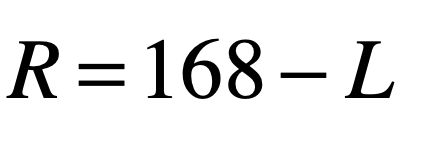
The Robinson Crusoe economy is one of the simplest economic models that captures the trade-off between labor and production on one side, and leisure and consumption on the other. The model has a single laborer for whom there are 24*7 =168 hours in the week. Some of these hours must be spent finding food, let’s say coconuts, while the other hours are for leisure and rest. The production of coconuts follows a production curve
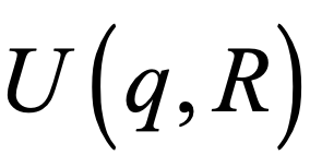
that is a function of labor L. There are diminishing returns in the finding of coconuts for a given labor, making the production curve of coconuts convex. The amount of rest is
and there is a reciprocal production curve q(R) related to less coconuts produced for more time spent resting. In this model it is assumed that all coconuts that are produced are consumed. This is known as market clearing when no surplus is built up.
The production curve presents a continuous trade-off between consumption and leisure, but at first look there is no obvious way to decide how much to work and how much to rest. A lazy person might be willing to go a little hungry if they can have more rest, while a busy person might want to use all waking hours to find coconuts. The production curve represents something known as a Pareto frontier. It is a continuous trade-off between two qualities. Another example of a Pareto frontier is car engine efficiency versus cost. Some consumers may care more about the up-front cost of the car than the cost of gas, while other consumers may value fuel efficiency and be willing to pay higher costs to get it.
Continuous trade offs always present a bit of a problem for planning. It is often not clear what the best trade off should be. This problem is solved by introducing another concept into this little economy–the concept of “Utility”.
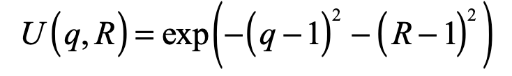
The utility function was introduced by the physicist Daniel Bernoulli, one of the many bountiful Bernoullis of Basel, in 1738. The utility function is a measure of how much benefit or utility a person or an enterprise gains by holding varying amounts of goods or labor. The essential problem in economic exchange is to maximize one’s utility function subject to whatever constraints are active. The utility function for Robinson Crusoe is
This function is obviously a maximum at maximum leisure (R = 1) and lots of coconuts (q = 1), but this is not allowed, because it lies off the production curve q(R). Therefore the question becomes: where on the production curve he can maximize the trade-off between coconuts and leisure?
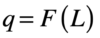
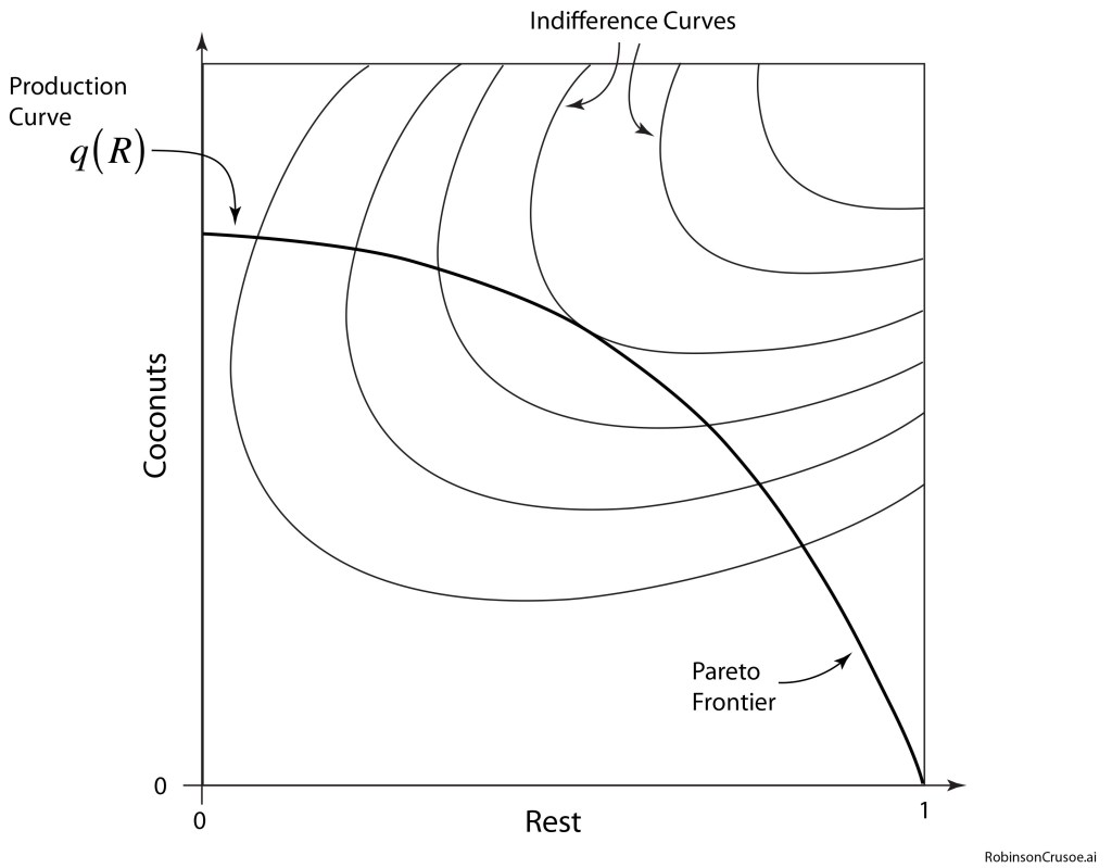
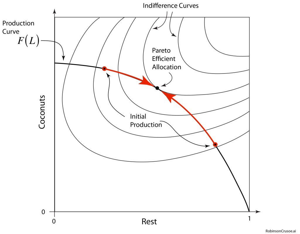
Fig. 1 shows the dynamical space for Robinson Crusoe’s economy. The space is two dimensional with axes for coconuts q and rest R. Isoclines of the utility function are shown as contours known as “indifference” curves, because the utility is constant along these curves and hence Robinson Crusoe is indifferent to his position on it. The indifference curves are cut by the production curve q(R). The equilibrium problem is to maximize utility subject to the production curve.
Fig. 1 The production space of the Robinson Crusoe economy. The production curve q(R) cuts across the isoclines of the utility function U(q,R). The contours represent “indifference” curves because the utility is constant along a contour.
When looking at dynamics under constraints, Lagrange multipliers are the best tool. Furthermore, we can impart dynamics into the model with temporal adjustments in q and R that respond to economic forces.
The Lagrangian Economy
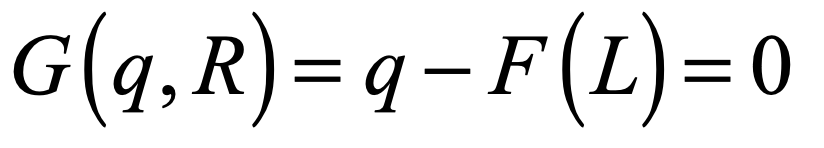
The approach to the Lagrangian economy is identical to the Lagrangian approach in classical physics. The equation of constraint is
All the dynamics take place on the production curve. The initial condition starts on the curve, and the state point moves along the curve until it reaches a maximum and settles into equilibrium. The dynamics is therefore one-dimensional, the link between q and R being the production curve.
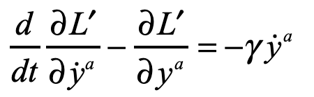
The Lagrangian in this simple economy is given by the utility function augmented by the equation of constraint, such that
where the term on the right-hand-side is a drag force with the relaxation rate γ.
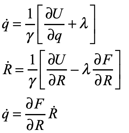
The first term on the left is the momentum of the system. In economic dynamics, this is usually negligible, similar to dynamics in living systems at low Reynold’s number in which all objects are moving instantaneously at their terminal velocity in response to forces. The equations of motion are therefore
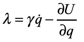
The Lagrange multiplier can be solved from the first equation as
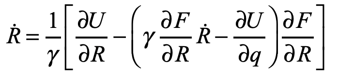
and the last equation converts q-dot to R-dot to yield the single equation
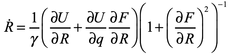
which is a one-dimensional flow
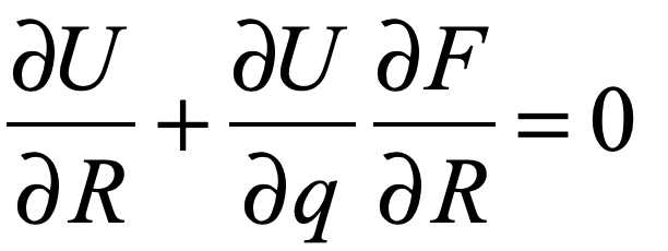
where all q’s are expressed as R’s through the equation of constraint. The speed vanishes at the fixed point—the economic equilibrium—when
This is the point of Pareto efficient allocation. Any initial condition on the production curve will relax to this point with a rate given by γ. These trajectories are shown in Fig. 2. From the point of view of Robinson Crusoe, if he is working harder than he needs, then he will slack off. But if there aren’t enough coconuts to make him happy, he will work harder.
Fig. 2 Motion occurs on the one-dimensional manifold defined by the production curve such that the utility is maximized at a unique point called the Pareto Efficient Allocation.
The production curve is like a curved wire, the amount of production q is like the bead sliding on the wire. The utility function plays the role of a potential function, and the gradients of the utility function play the role of forces. Then this simple economic model is just like ordinary classical physics of point masses responding to forces constrained to lie on certain lines or surfaces. From this viewpoint, physics and economics are literally the same.
Worked Example
To make this problem specific, consider a utility function given by
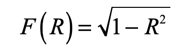
that has a maximum in the upper right corner, and a production curve given by
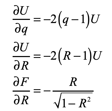
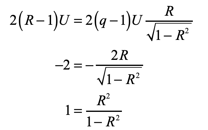
that has diminishing returns. Then, the condition of equilibrium can be solved using
to yield
With the (fairly obvious) answer
By David D. Nolte, Feb. 10, 2022
For More Reading
[1] D. D. Nolte, Introduction to Modern Dynamics : Chaos, Networks, Space and Time, 2nd ed. Oxford : Oxford University Press (2019).
[2] Fritz Söllner; The Use (and Abuse) of Robinson Crusoe in Neoclassical Economics. History of Political Economy; 48 (1): 35–64. (2016)
Nature loves the path of steepest descent. Place a ball on a smooth curved surface and release it, and it will instantansouly accelerate in the direction of steepest descent. Shoot a laser beam from an oblique angle onto a piece of glass to hit a target inside, and the path taken by the beam is the only path that decreases the distance to the target in the shortest time. Diffract a stream of electrons from the surface of a crystal, and quantum detection events are greatest at the positions where the troughs and peaks of the deBroglie waves converge the most. The first example is Newton’s second law. The second example is Fermat’s principle and Snell’s Law. The third example is Feynman’s path-integral formulation of quantum mechanics. They all share in common a minimization principle—the principle of least action—that the path of a dynamical system is the one that minimizes a property known as “action”.
The Eikonal Equation is the “F = ma” of ray optics. It’s solutions describe the paths of light rays through complicated media.
The principle of least action, first proposed by the French physicist Maupertuis through mechanical analogy, became a principle of Lagrangian mechanics in the hands of Lagrange, but was still restricted to mechanical systems of particles. The principle was generalized forty years later by Hamilton, who began by considering the propagation of light waves, and ended by transforming mechanics into a study of pure geometry divorced from forces and inertia. Optics played a key role in the development of mechanics, and mechanics returned the favor by giving optics the Eikonal Equation. The Eikonal Equation is the “F = ma” of ray optics. It’s solutions describe the paths of light rays through complicated media.
Malus’ Theorem
Anyone who has taken a course in optics knows that Étienne-Louis Malus (1775-1812) discovered the polarization of light, but little else is taught about this French mathematician who was one of the savants Napoleon had taken along with himself when he invaded Egypt in 1798. After experiencing numerous horrors of war and plague, Malus returned to France damaged but wiser. He discovered the polarization of light in the Fall of 1808 as he was playing with crystals of icelandic spar at sunset and happened to view last rays of the sun reflected from the windows of the Luxumbourg palace. Icelandic spar produces double images in natural light because it is birefringent. Malus discovered that he could extinguish one of the double images of the Luxumbourg windows by rotating the crystal a certain way, demonstrating that light is polarized by reflection. The degree to which light is extinguished as a function of the angle of the polarizing crystal is known as Malus’ Law.
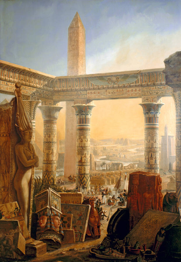
Fronts-piece to the Description de l’Égypte , the first volume published by Joseph Fourier in 1808 based on the report of the savants of L’Institute de l’Égypte that included Monge, Fourier and Malus, among many other French scientists and engineers.
Malus had picked up an interest in the general properties of light and imaging during lulls in his ordeal in Egypt. (To read about Malus’ misadventures during Napoleon’s campaign in Egypt, see Chapter 1 of Interference.) He was an emissionist following his compatriot Laplace, rather than an undulationist following Thomas Young. It is ironic that the French scientists were staunchly supporting Newton on the nature of light, while the British scientist Thomas Young was trying to upend Netwonian optics. Almost all physicists at that time were emissionists, only a few years after Young’s double-slit experiment of 1804, and few serious scientists accepted Young’s theory of the wave nature of light until Fresnel and Arago supplied the rigorous theory and experimental proofs much later in 1819.
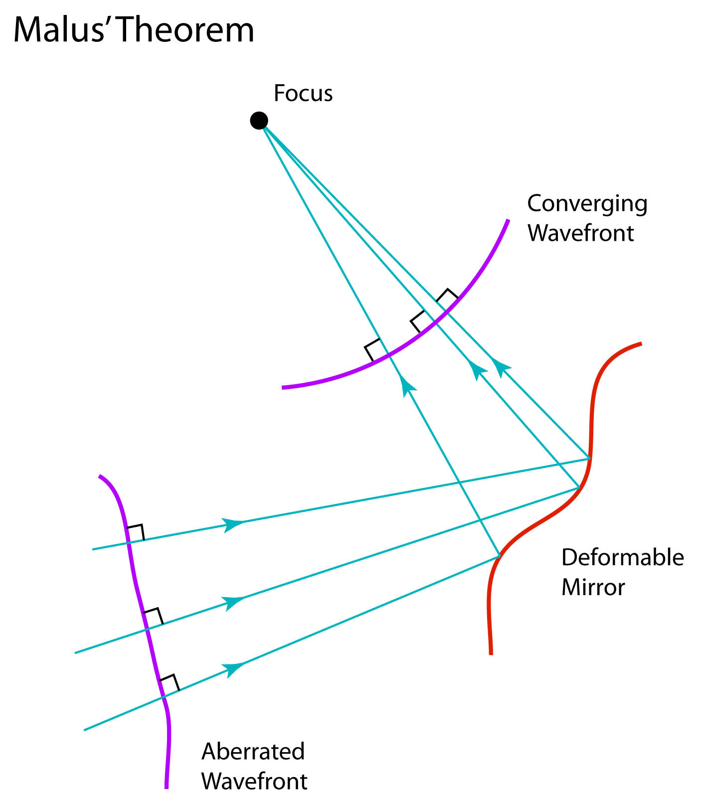
Malus’ Theorem states that rays perpendicular to an initial surface are perpendicular to a later surface after reflection in an optical system. This theorem is the starting point for the Eikonal ray equation, as well as for modern applications in adaptive optics. This figure shows a propagating aberrated wavefront that is “compensated” by a deformable mirror to produce a tight focus.
As a prelude to his later discovery of polarization, Malus had earlier proven a theorem about trajectories that particles of light take through an optical system. One of the key questions about the particles of light in an optical system was how they formed images. The physics of light particles moving through lenses was too complex to treat at that time, but reflection was relatively easy based on the simple reflection law. Malus proved a theorem mathematically that after a reflection from a curved mirror, a set of rays perpendicular to an initial nonplanar surface would remain perpendicular at a later surface after reflection (this property is closely related to the conservation of optical etendue). This is known as Malus’ Theorem, and he thought it only held true after a single reflection, but later mathematicians proved that it remains true even after an arbitrary number of reflections, even in cases when the rays intersect to form an optical effect known as a caustic. The mathematics of caustics would catch the interest of an Irish mathematician and physicist who helped launch a new field of mathematical physics.
Etienne-Louis Malus
Hamilton’s Characteristic Function
William Rowan Hamilton (1805 – 1865) was a child prodigy who taught himself thirteen languages by the time he was thirteen years old (with the help of his linguist uncle), but mathematics became his primary focus at Trinity College at the University in Dublin. His mathematical prowess was so great that he was made the Astronomer Royal of Ireland while still an undergraduate student. He also became fascinated in the theory of envelopes of curves and in particular to the mathematics of caustic curves in optics.
In 1823 at the age of 18, he wrote a paper titled Caustics that was read to the Royal Irish Academy. In this paper, Hamilton gave an exceedingly simple proof of Malus’ Law, but that was perhaps the simplest part of the paper. Other aspects were mathematically obscure and reviewers requested further additions and refinements before publication. Over the next four years, as Hamilton expanded this work on optics, he developed a new theory of optics, the first part of which was published as Theory of Systems of Rays in 1827 with two following supplements completed by 1833 but never published.
Hamilton’s most important contribution
to optical theory (and eventually to mechanics) he called his characteristic
function. By applying the principle of
Fermat’s least time, which he called his principle of stationary action, he
sought to find a single unique function that characterized every path through
an optical system. By first proving
Malus’ Theorem and then applying the theorem to any system of rays using the
principle of stationary action, he was able to construct two partial
differential equations whose solution, if it could be found, defined every ray
through the optical system. This result
was completely general and could be extended to include curved rays passing
through inhomogeneous media. Because it
mapped input rays to output rays, it was the most general characterization of
any defined optical system. The
characteristic function defined surfaces of constant action whose normal
vectors were the rays of the optical system.
Today these surfaces of constant action are called the Eikonal function
(but how it got its name is the next chapter of this story). Using his characteristic function, Hamilton
predicted a phenomenon known as conical refraction in 1832, which was
subsequently observed, launching him to a level of fame unusual for an
academic.
Once Hamilton had established his principle of stationary action of curved light rays, it was an easy step to extend it to apply to mechanical systems of particles with curved trajectories. This step produced his most famous work On a General Method in Dynamics published in two parts in 1834 and 1835 [1] in which he developed what became known as Hamiltonian dynamics. As his mechanical work was extended by others including Jacobi, Darboux and Poincaré, Hamilton’s work on optics was overshadowed, overlooked and eventually lost. It was rediscovered when Schrödinger, in his famous paper of 1926, invoked Hamilton’s optical work as a direct example of the wave-particle duality of quantum mechanics [2]. Yet in the interim, a German mathematician tackled the same optical problems that Hamilton had seventy years earlier, and gave the Eikonal Equation its name.
Bruns’ Eikonal
The German mathematician Heinrich Bruns (1848-1919) was engaged chiefly with the measurement of the Earth, or geodesy. He was a professor of mathematics in Berlin and later Leipzig. One claim fame was that one of his graduate students was Felix Hausdorff [3] who would go on to much greater fame in the field of set theory and measure theory (the Hausdorff dimension was a precursor to the fractal dimension). Possibly motivated by his studies done with Hausdorff on refraction of light by the atmosphere, Bruns became interested in Malus’ Theorem for the same reasons and with the same goals as Hamilton, yet was unaware of Hamilton’s work in optics.
The mathematical process of creating “images”, in the sense of a mathematical mapping, made Bruns think of the Greek word εικων which literally means “icon” or “image”, and he published a small book in 1895 with the title Das Eikonal in which he derived a general equation for the path of rays through an optical system. His approach was heavily geometrical and is not easily recognized as an equation arising from variational principals. It rediscovered most of the results of Hamilton’s paper on the Theory of Systems of Rays and was thus not groundbreaking in the sense of new discovery. But it did reintroduce the world to the problem of systems of rays, and his name of Eikonal for the equations of the ray paths stuck, and was used with increasing frequency in subsequent years. Arnold Sommerfeld (1868 – 1951) was one of the early proponents of the Eikonal equation and recognized its connection with action principles in mechanics. He discussed the Eikonal equation in a 1911 optics paper with Runge [4] and in 1916 used action principles to extend Bohr’s model of the hydrogen atom [5]. While the Eikonal approach was not used often, it became popular in the 1960’s when computational optics made numerical solutions possible.
Lagrangian Dynamics of Light Rays
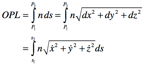
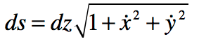
In physical optics, one of the most important properties of a ray passing through an optical system is known as the optical path length (OPL). The OPL is the central quantity that is used in problems of interferometry, and it is the central property that appears in Fermat’s principle that leads to Snell’s Law. The OPL played an important role in the history of the calculus when Johann Bernoulli in 1697 used it to derive the path taken by a light ray as an analogy of a brachistochrone curve – the curve of least time taken by a particle between two points.
The OPL between two points in a refractive medium is the sum of the piecewise product of the refractive index n with infinitesimal elements of the path length ds. In integral form, this is expressed as
where the “dot” is a derivative
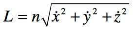
with respedt to s. The optical
Lagrangian is recognized as
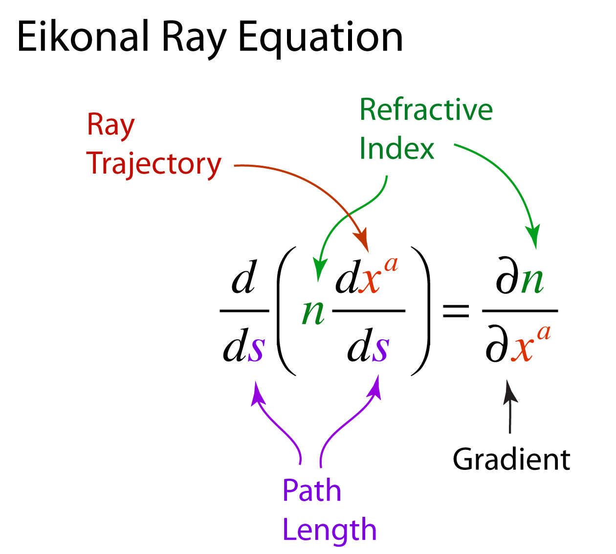
The Lagrangian is inserted into the Euler equations to yield (after some algebra, see Introduction to Modern Dynamics pg. 336)
This is a second-order
ordinary differential equation in the variables xa that define the
ray path through the system. It is
literally a “trajectory” of the ray, and the Eikonal equation becomes the F =
ma of ray optics.
Hamiltonian Optics
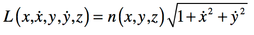
In a paraxial system (in which
the rays never make large angles relative to the optic axis) it is common to
select the position z as a single parameter to define the curve of the ray path
so that the trajectory is parameterized as
where the derivatives
are with respect to z, and the effective Lagrangian is recognized as
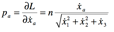
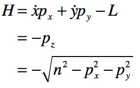
The Hamiltonian
formulation is derived from the Lagrangian by defining an optical Hamiltonian
as the Legendre transform of the Lagrangian.
To start, the Lagrangian is expressed in terms of the generalized
coordinates and momenta. The generalized
optical momenta are defined as
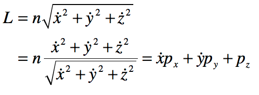
This relationship leads
to an alternative expression for the Eikonal equation (also known as the scalar
Eikonal equation) expressed as
where S(x,y,z) = const. is the eikonal function. The
momentum vectors are perpendicular to the surfaces of constant S, which
are recognized as the wavefronts of a propagating wave.
The
Lagrangian can be restated as a function of the generalized momenta as
and the Legendre
transform that takes the Lagrangian into the Hamiltonian is
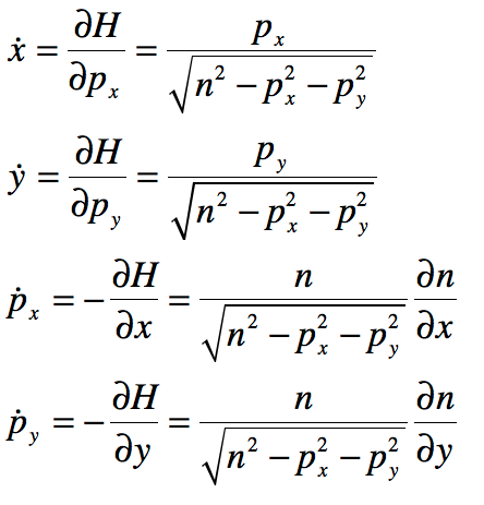
The trajectory of the
rays is the solution to Hamilton’s equations of motion applied to this
Hamiltonian
Light Orbits
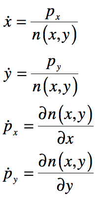
If the optical rays are
restricted to the x-y plane, then Hamilton’s equations of motion can be
expressed relative to the path length ds, and the momenta are pa =
ndxa/ds. The ray equations are
(simply expressing the 2 second-order Eikonal equation as 4 first-order
equations)
where the dot is a derivative
with respect to the element ds.
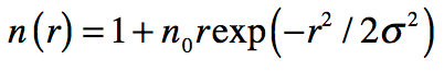
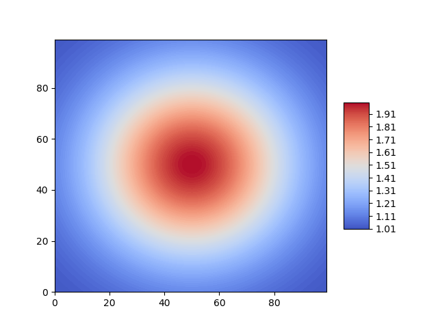
As an example, consider a radial refractive index profile in the x-y plane
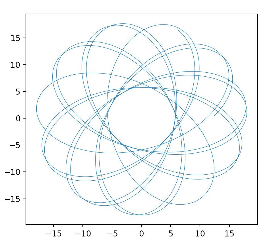
where r is the radius on the x-y plane. Putting this refractive index profile into the Eikonal equations creates a two-dimensional orbit in the x-y plane. The Eikonal Equation is the “F = ma” of ray optics. It’s solutions describe the paths of light rays through complicated media, including the phenomenon of gravitational lensing (see my blog post) and the orbits of photons around black holes (see my other blog post).
By David D. Nolte, May 30, 2019
Gaussian refractive index profile in the x-y plane. From raysimple.py.
Ray orbits around the center of the Gaussian refractive index profile. From raysimple.py
Python Code: raysimple.py
The following Python code solves for individual trajectories. (Python code on GitHub.)
#!/usr/bin/env python3
# -*- coding: utf-8 -*-
"""
raysimple.py
Created on Tue May 28 11:50:24 2019
@author: nolte
D. D. Nolte, Introduction to Modern Dynamics: Chaos, Networks, Space and Time, 2nd ed. (Oxford,2019)
"""

import numpy as np
import matplotlib as mpl
from mpl_toolkits.mplot3d import Axes3D
from scipy import integrate
from matplotlib import pyplot as plt
from matplotlib import cm
import time
import os

plt.close('all')

# selection 1 = Gaussian
# selection 2 = Donut
selection = 1

print(' ')
print('raysimple.py')

def refindex(x,y):

    if selection == 1:

        sig = 10

        n = 1 + np.exp(-(x**2 + y**2)/2/sig**2)
        nx = (-2*x/2/sig**2)*np.exp(-(x**2 + y**2)/2/sig**2)
        ny = (-2*y/2/sig**2)*np.exp(-(x**2 + y**2)/2/sig**2)

    elif selection == 2:

        sig = 10;
        r2 = (x**2 + y**2)
        r1 = np.sqrt(r2)
        np.expon = np.exp(-r2/2/sig**2)

        n = 1+0.3*r1*np.expon;
        nx = 0.3*r1*(-2*x/2/sig**2)*np.expon + 0.3*np.expon*2*x/r1
        ny = 0.3*r1*(-2*y/2/sig**2)*np.expon + 0.3*np.expon*2*y/r1


    return [n,nx,ny]


def flow_deriv(x_y_z,tspan):
    x, y, z, w = x_y_z

    n, nx, ny = refindex(x,y)

    yp = np.zeros(shape=(4,))
    yp[0] = z/n
    yp[1] = w/n
    yp[2] = nx
    yp[3] = ny

    return yp

V = np.zeros(shape=(100,100))
for xloop in range(100):
    xx = -20 + 40*xloop/100
    for yloop in range(100):
        yy = -20 + 40*yloop/100
        n,nx,ny = refindex(xx,yy)
        V[yloop,xloop] = n

fig = plt.figure(1)
contr = plt.contourf(V,100, cmap=cm.coolwarm, vmin = 1, vmax = 3)
fig.colorbar(contr, shrink=0.5, aspect=5)
fig = plt.show()


v1 = 0.707      # Change this initial condition
v2 = np.sqrt(1-v1**2)
y0 = [12, 0, v1, v2]     # Change these initial conditions

tspan = np.linspace(1,1700,1700)

y = integrate.odeint(flow_deriv, y0, tspan)

plt.figure(2)
lines = plt.plot(y[1:1550,0],y[1:1550,1])
plt.setp(lines, linewidth=0.5)
plt.show()
New from Oxford University Press: Interference and the History of Light and Optics (2023)
Read the stories of the scientists and engineers who tamed light and used it to probe the universe.
An excellent textbook on geometric optics from Hamilton’s point of view is K. B. Wolf, Geometric Optics in Phase Space (Springer, 2004). Another is H. A. Buchdahl, An Introduction to Hamiltonian Optics (Dover, 1992).
A rather older textbook on geometrical optics is by J. L. Synge, Geometrical Optics: An Introduction to Hamilton’s Method (Cambridge University Press, 1962) showing the derivation of the ray equations in the final chapter using variational methods. Synge takes a dim view of Bruns’ term “Eikonal” since Hamilton got there first and Bruns was unaware of it.
A book that makes an especially strong case for the Optical-Mechanical analogy of Fermat’s principle, connecting the trajectories of mechanics to the paths of optical rays is Daryl Holm, Geometric Mechanics: Part I Dynamics and Symmetry (Imperial College Press 2008).
[1] Hamilton, W. R. “On a general method in dynamics I.” Mathematical Papers, I ,103-161: 247-308. (1834); Hamilton, W. R. “On a general method in dynamics II.” Mathematical Papers, I ,103-161: 95-144. (1835)
[2] Schrodinger, E. “Quantification of the eigen-value problem.” Annalen Der Physik 79(6): 489-527. (1926)