The Physics of Robinson Crusoe’s Economy

“What is a coconut worth to a cast-away on a deserted island?”

In the midst of the cast-away’s misfortune and hunger and exertion and food lies an answer that looks familiar to any physicist who speaks the words

“Assume a Lagrangian …”

It is the same process that determines how a bead slides along a bent wire in gravity or a skier navigates a ski hill.  The answer: find the balance of economic forces subject to constraints. 

Here is the history and the physics behind one of the simplest economic systems that can be conceived:  Robinson Crusoe spending his time collecting coconuts!

Robinson Crusoe in Economic History

Daniel Defoe published “The Life and Strange Surprizing Adventures of Robinson Crusoe” in 1719, about a man who is shipwrecked on a deserted island and survives there for 28 years before being rescued.  It was written in the first person, as if the author had actually lived through those experiences, and it was based on a real-life adventure story.  It is one of the first examples of realistic fiction, and it helped establish the genre of the English novel.

Several writers on economic theory made mention of Robinson Crusoe as an example of a labor economy, but it was in 1871 that Robinson Crusoe became an economic archetype.  In that year both William Stanley Jevons‘s The Theory of Political Economy and Carl Menger‘s Grundsätze der Volkswirtschaftslehre (Principles of Economics) used Robinson Crusoe to illustrate key principles of the budding marginalist revolution.

Marginalism in economic theory is the demarcation between classical economics and modern economics.  The key principle of marginalism is the principle of “diminishing returns” as the value of something gets less as an individual has more of it.  This principle makes functions convex, which helps to guarantee that there are equilibrium points in the economy.  Economic equilibrium is a key concept and goal because it provides stability to economic systems.

One-Product Is a Dull Diet

The Robinson Crusoe economy is  one of the simplest economic models that captures the trade-off between labor and production on one side, and leisure and consumption on the other.  The model has a single laborer for whom there are 24*7 =168 hours in the week.  Some of these hours must be spent finding food, let’s say coconuts, while the other hours are for leisure and rest.  The production of coconuts follows a production curve

that is a function of labor L.  There are diminishing returns in the finding of coconuts for a given labor, making the production curve of coconuts convex.  The amount of rest is

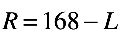
and there is a reciprocal production curve q(R) related to less coconuts produced for more time spent resting. In this model it is assumed that all coconuts that are produced are consumed.  This is known as market clearing when no surplus is built up. 

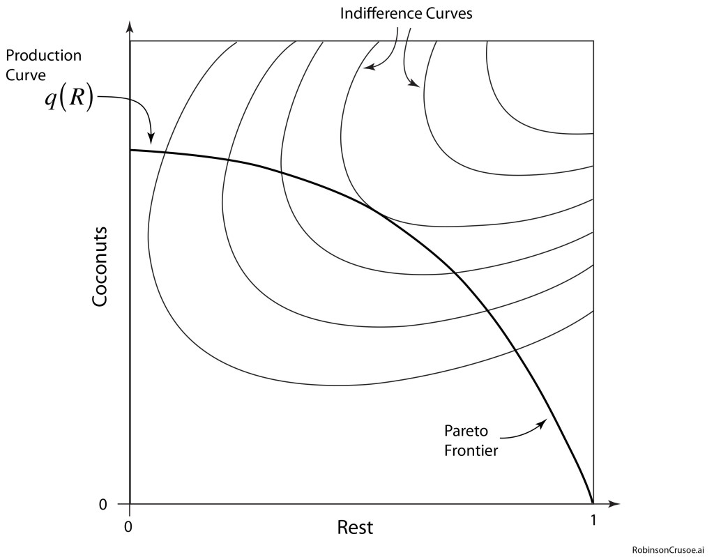
The production curve presents a continuous trade-off between consumption and leisure, but at first look there is no obvious way to decide how much to work and how much to rest.  A lazy person might be willing to go a little hungry if they can have more rest, while a busy person might want to use all waking hours to find coconuts.  The production curve represents something known as a Pareto frontier.  It is a continuous trade-off between two qualities.  Another example of a Pareto frontier is car engine efficiency versus cost.  Some consumers may care more about the up-front cost of the car than the cost of gas, while other consumers may value fuel efficiency and be willing to pay higher costs to get it. 

Continuous trade offs always present a bit of a problem for planning. It is often not clear what the best trade off should be. This problem is solved by introducing another concept into this little economy–the concept of “Utility”.

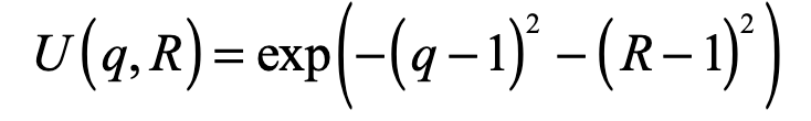
The utility function was introduced by the physicist Daniel Bernoulli, one of the many bountiful Bernoullis of Basel, in 1738. The utility function is a measure of how much benefit or utility a person or an enterprise gains by holding varying amounts of goods or labor. The essential problem in economic exchange is to maximize one’s utility function subject to whatever constraints are active. The utility function for Robinson Crusoe is

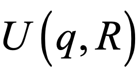
This function is obviously a maximum at maximum leisure (R = 1) and lots of coconuts (q = 1), but this is not allowed, because it lies off the production curve q(R). Therefore the question becomes: where on the production curve he can maximize the trade-off between coconuts and leisure?

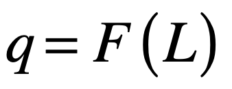
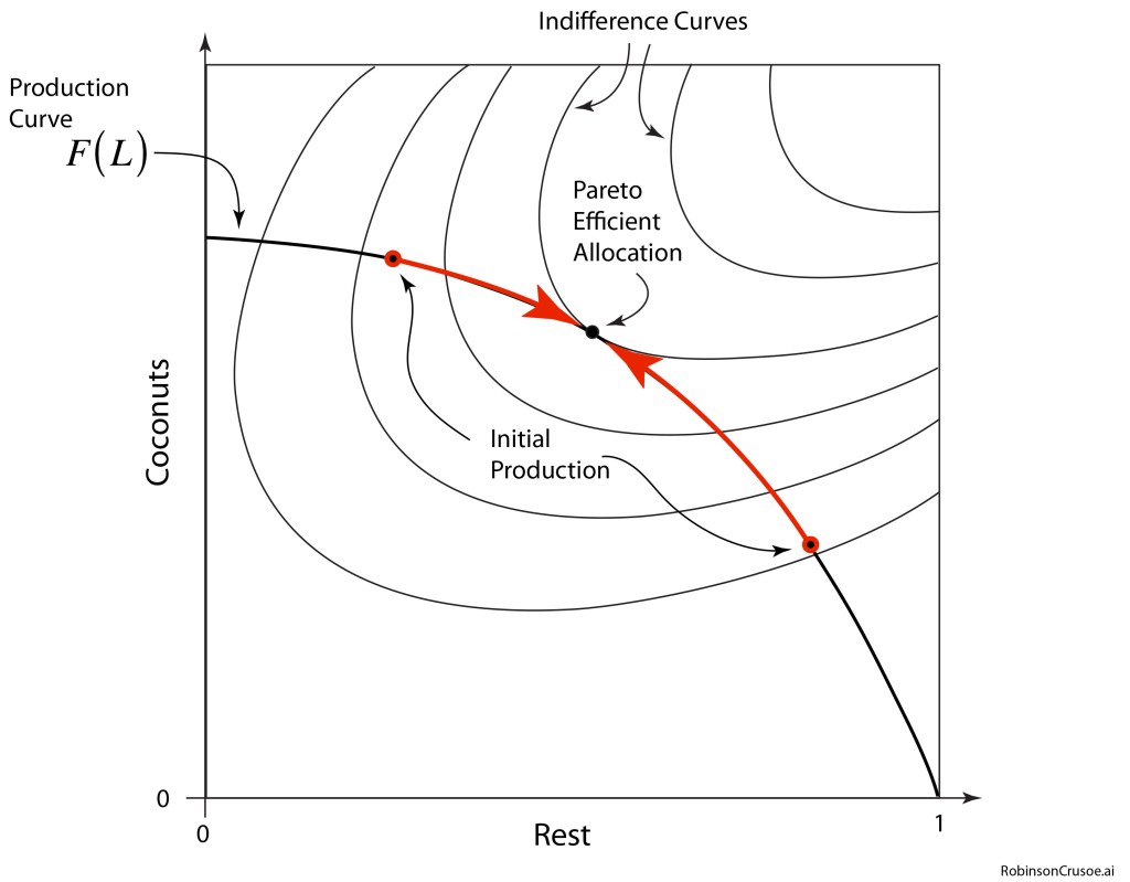
Fig. 1 shows the dynamical space for Robinson Crusoe’s economy. The space is two dimensional with axes for coconuts q and rest R. Isoclines of the utility function are shown as contours known as “indifference” curves, because the utility is constant along these curves and hence Robinson Crusoe is indifferent to his position on it. The indifference curves are cut by the production curve q(R). The equilibrium problem is to maximize utility subject to the production curve.

Fig. 1 The production space of the Robinson Crusoe economy. The production curve q(R) cuts across the isoclines of the utility function U(q,R). The contours represent “indifference” curves because the utility is constant along a contour.

When looking at dynamics under constraints, Lagrange multipliers are the best tool. Furthermore, we can impart dynamics into the model with temporal adjustments in q and R that respond to economic forces.

The Lagrangian Economy

The approach to the Lagrangian economy is identical to the Lagrangian approach in classical physics. The equation of constraint is

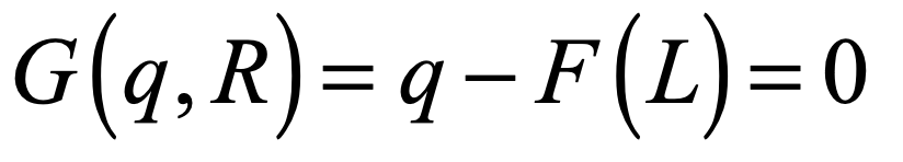
All the dynamics take place on the production curve. The initial condition starts on the curve, and the state point moves along the curve until it reaches a maximum and settles into equilibrium. The dynamics is therefore one-dimensional, the link between q and R being the production curve.

The Lagrangian in this simple economy is given by the utility function augmented by the equation of constraint, such that

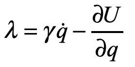
where λ is the Lagrangian undetermined multiplier. The Euler-Lagrange equations for dynamics are

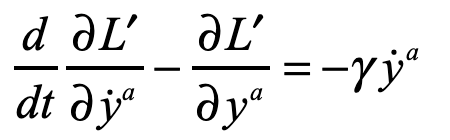
where the term on the right-hand-side is a drag force with the relaxation rate γ.

The first term on the left is the momentum of the system. In economic dynamics, this is usually negligible, similar to dynamics in living systems at low Reynold’s number in which all objects are moving instantaneously at their terminal velocity in response to forces. The equations of motion are therefore

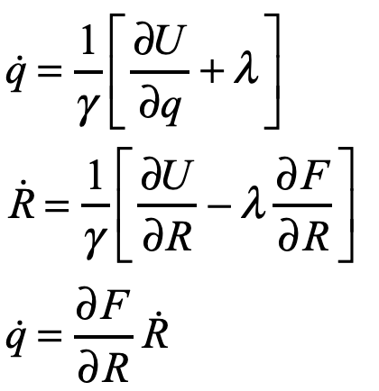
The Lagrange multiplier can be solved from the first equation as

and the last equation converts q-dot to R-dot to yield the single equation

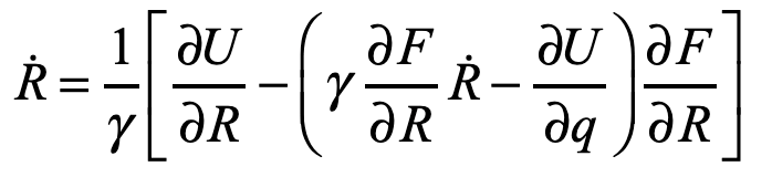
which is a one-dimensional flow

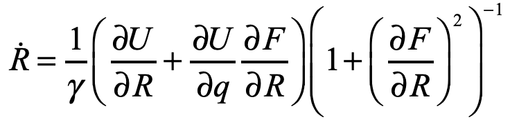
where all q’s are expressed as R’s through the equation of constraint. The speed vanishes at the fixed point—the economic equilibrium—when

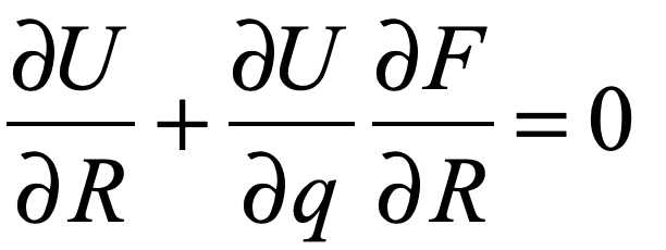
This is the point of Pareto efficient allocation. Any initial condition on the production curve will relax to this point with a rate given by γ. These trajectories are shown in Fig. 2. From the point of view of Robinson Crusoe, if he is working harder than he needs, then he will slack off. But if there aren’t enough coconuts to make him happy, he will work harder.

Fig. 2 Motion occurs on the one-dimensional manifold defined by the production curve such that the utility is maximized at a unique point called the Pareto Efficient Allocation.

The production curve is like a curved wire, the amount of production q is like the bead sliding on the wire. The utility function plays the role of a potential function, and the gradients of the utility function play the role of forces. Then this simple economic model is just like ordinary classical physics of point masses responding to forces constrained to lie on certain lines or surfaces. From this viewpoint, physics and economics are literally the same.

Worked Example

To make this problem specific, consider a utility function given by

that has a maximum in the upper right corner, and a production curve given by

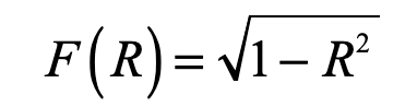
that has diminishing returns. Then, the condition of equilibrium can be solved using
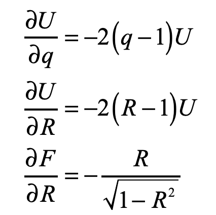
to yield

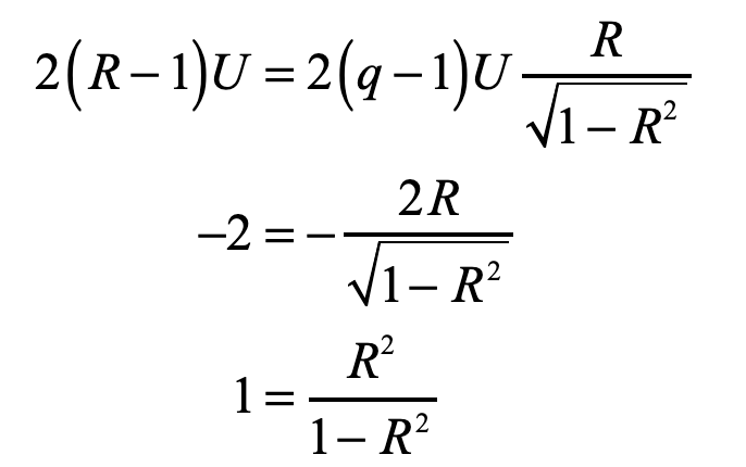
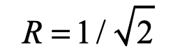
With the (fairly obvious) answer

By David D. Nolte, Feb. 10, 2022

For More Reading

[1] D. D. Nolte, Introduction to Modern Dynamics : Chaos, Networks, Space and Time, 2nd ed. Oxford : Oxford University Press (2019).

[2] Fritz Söllner; The Use (and Abuse) of Robinson Crusoe in Neoclassical Economics. History of Political Economy; 48 (1): 35–64. (2016)

Second Edition of Introduction to Modern Dynamics (Chaos, Networks, Space and Time)

The second edition of Introduction to Modern Dynamics: Chaos, Networks, Space and Time is available from Oxford University Press and Amazon.

Most physics majors will use modern dynamics in their careers: nonlinearity, chaos, network theory, econophysics, game theory, neural nets, geodesic geometry, among many others.

The first edition of Introduction to Modern Dynamics (IMD) was an upper-division junior-level mechanics textbook at the level of Thornton and Marion (Classical Dynamics of Particles and Systems) and Taylor (Classical Mechanics).  IMD helped lead an emerging trend in physics education to update the undergraduate physics curriculum.  Conventional junior-level mechanics courses emphasized Lagrangian and Hamiltonian physics, but notably missing from the classic subjects are modern dynamics topics that most physics majors will use in their careers: nonlinearity, chaos, network theory, econophysics, game theory, neural nets, geodesic geometry, among many others.  These are the topics at the forefront of physics that drive high-tech businesses and start-ups, which is where more than half of all physicists work. IMD introduced these modern topics to junior-level physics majors in an accessible form that allowed them to master the fundamentals to prepare them for the modern world.

The second edition (IMD2) continues that trend by expanding the chapters to include additional material and topics.  It rearranges several of the introductory chapters for improved logical flow and expands them to include key conventional topics that were missing in the first edition (e.g., Lagrange undetermined multipliers and expanded examples of Lagrangian applications).  It is also an opportunity to correct several typographical errors and other errata that students have identified over the past several years.  The second edition also has expanded homework problems.

The goal of IMD2 is to strengthen the sections on conventional topics (that students need to master to take their GREs) to make IMD2 attractive as a mainstream physics textbook for broader adoption at the junior level, while continuing the program of updating the topics and approaches that are relevant for the roles that physicists play in the 21st century.

(New Chapters and Sections highlighted in red.)

New Features in Second Edition:

Second Edition Chapters and Sections

Part 1 Geometric Mechanics

• Expanded development of Lagrangian dynamics

• Lagrange multipliers

• More examples of applications

• Connection to statistical mechanics through the virial theorem

• Greater emphasis on action-angle variables

• The key role of adiabatic invariants

Part 1 Geometric Mechanics

Chapter 1 Physics and Geometry

1.1 State space and dynamical flows

1.2 Coordinate representations

1.3 Coordinate transformation

1.4 Uniformly rotating frames

1.5 Rigid-body motion

Chapter 2 Lagrangian Mechanics

2.1 Calculus of variations

2.2 Lagrangian applications

2.3 Lagrange’s undetermined multipliers

2.4 Conservation laws

2.5 Central force motion

2.6 Virial Theorem

Chapter 3 Hamiltonian Dynamics and Phase Space

3.1 The Hamiltonian function

3.2 Phase space

3.3 Integrable systems and action–angle variables

3.4 Adiabatic invariants

Part 2 Nonlinear Dynamics

• New section on non-autonomous dynamics

• Entire new chapter devoted to Hamiltonian mechanics

• Added importance to Chirikov standard map

• The important KAM theory of “constrained chaos” and solar system stability

• Degeneracy in Hamiltonian chaos

• A short overview of quantum chaos

• Rational resonances and the relation to KAM theory

• Synchronized chaos

Part 2 Nonlinear Dynamics

Chapter 4 Nonlinear Dynamics and Chaos

4.1 One-variable dynamical systems

4.2 Two-variable dynamical systems

4.3 Limit cycles

4.4 Discrete iterative maps

4.5 Three-dimensional state space and chaos

4.6 Non-autonomous (driven) flows

4.7 Fractals and strange attractors

Chapter 5 Hamiltonian Chaos

5.1 Perturbed Hamiltonian systems

5.2 Nonintegrable Hamiltonian systems

5.3 The Chirikov Standard Map

5.4 KAM Theory

5.5 Degeneracy and the web map

5.6 Quantum chaos

Chapter 6 Coupled Oscillators and Synchronization

6.1 Coupled linear oscillators

6.2 Simple models of synchronization

6.3 Rational resonances

6.4 External synchronization

6.5 Synchronization of Chaos

Part 3 Complex Systems

• New emphasis on diffusion on networks

• Epidemic growth on networks

• A new section of game theory in the context of evolutionary dynamics

• A new section on general equilibrium theory in economics

Part 3 Complex Systems

Chapter 7 Network Dynamics

7.1 Network structures

7.2 Random network topologies

7.3 Synchronization on networks

7.4 Diffusion on networks

7.5 Epidemics on networks

Chapter 8 Evolutionary Dynamics

81 Population dynamics

8.2 Virus infection and immune deficiency

8.3 Replicator Dynamics

8.4 Quasi-species

8.5 Game theory and evolutionary stable solutions

Chapter 9 Neurodynamics and Neural Networks

9.1 Neuron structure and function

9.2 Neuron dynamics

9.3 Network nodes: artificial neurons

9.4 Neural network architectures

9.5 Hopfield neural network

9.6 Content-addressable (associative) memory

Chapter 10 Economic Dynamics

10.1 Microeconomics and equilibrium

10.2 Macroeconomics

10.3 Business cycles

10.4 Random walks and stock prices (optional)

Part 4 Relativity and Space–Time

• Relativistic trajectories

• Gravitational waves

Part 4 Relativity and Space–Time

Chapter 11 Metric Spaces and Geodesic Motion

11.1 Manifolds and metric tensors

11.2 Derivative of a tensor

11.3 Geodesic curves in configuration space

11.4 Geodesic motion

Chapter 12 Relativistic Dynamics

12.1 The special theory

12.2 Lorentz transformations

12.3 Metric structure of Minkowski space

12.4 Relativistic trajectories

12.5 Relativistic dynamics

12.6 Linearly accelerating frames (relativistic)

Chapter 13 The General Theory of Relativity and Gravitation

13.1 Riemann curvature tensor

13.2 The Newtonian correspondence

13.3 Einstein’s field equations

13.4 Schwarzschild space–time

13.5 Kinematic consequences of gravity

13.6 The deflection of light by gravity

13.7 The precession of Mercury’s perihelion

13.8 Orbits near a black hole

13.9 Gravitational waves

Synopsis of 2nd Ed. Chapters

Chapter 1. Physics and Geometry (Sample Chapter)

This chapter has been rearranged relative to the 1st edition to provide a more logical flow of the overarching concepts of geometric mechanics that guide the subsequent chapters.  The central role of coordinate transformations is strengthened, as is the material on rigid-body motion with expanded examples.

Chapter 2. Lagrangian Mechanics (Sample Chapter)

Much of the structure and material is retained from the 1st edition while adding two important sections.  The section on applications of Lagrangian mechanics adds many direct examples of the use of Lagrange’s equations of motion.  An additional new section covers the important topic of Lagrange’s undetermined multipliers

Chapter 3. Hamiltonian Dynamics and Phase Space (Sample Chapter)

The importance of Hamiltonian systems and dynamics merits a stand-alone chapter.  The topics from the 1st edition are expanded in this new chapter, including a new section on adiabatic invariants that plays an important role in the development of quantum theory.  Some topics are de-emphasized from the 1st edition, such as general canonical transformations and the symplectic structure of phase space, although the specific transformation to action-angle coordinates is retained and amplified.

Chapter 4. Nonlinear Dynamics and Chaos

The first part of this chapter is retained from the 1st edition with numerous minor corrections and updates of figures.  The second part of the IMD 1st edition, treating Hamiltonian chaos, will be expanded into the new Chapter 5.

Chapter 5. Hamiltonian Chaos

This new stand-alone chapter expands on the last half of Chapter 3 of the IMD 1st edition.  The physical character of Hamiltonian chaos is substantially distinct from dissipative chaos that it deserves its own chapter.  It is also a central topic of interest for complex systems that are either conservative or that have integral invariants, such as our N-body solar system that played such an important role in the history of chaos theory beginning with Poincaré.  The new chapter highlights Poincaré’s homoclinic tangle, illustrated by the Chirikov Standard Map.  The Standard Map is an excellent introduction to KAM theory, which is one of the crowning achievements of the theory of dynamical systems by Komogorov, Arnold and Moser, connecting to deeper aspects of synchronization and rational resonances that drive the structure of systems as diverse as the rotation of the Moon and the rings of Saturn.  This is also a perfect lead-in to the next chapter on synchronization.  An optional section at the end of this chapter briefly discusses quantum chaos to show how Hamiltonian chaos can be extended into the quantum regime.

Chapter 6. Synchronization

This is an updated version of the IMD 1st ed. chapter.  It has a reduced initial section on coupled linear oscillators, retaining the key ideas about linear eigenmodes but removing some irrelevant details in the 1st edition.  A new section is added that defines and emphasizes the importance of quasi-periodicity.  A new section on the synchronization of chaotic oscillators is added.

Chapter 7. Network Dynamics

This chapter rearranges the structure of the chapter from the 1st edition, moving synchronization on networks earlier to connect from the previous chapter.  The section on diffusion and epidemics is moved to the back of the chapter and expanded in the 2nd edition into two separate sections on these topics, adding new material on discrete matrix approaches to continuous dynamics.

Chapter 8. Neurodynamics and Neural Networks

This chapter is retained from the 1st edition with numerous minor corrections and updates of figures.

Chapter 9. Evolutionary Dynamics

Two new sections are added to this chapter.  A section on game theory and evolutionary stable solutions introduces core concepts of evolutionary dynamics that merge well with the other topics of the chapter such as the pay-off matrix and replicator dynamics.  A new section on nearly neutral networks introduces new types of behavior that occur in high-dimensional spaces which are counter intuitive but important for understanding evolutionary drift.

Chapter 10.  Economic Dynamics

This chapter will be significantly updated relative to the 1st edition.  Most of the sections will be rewritten with improved examples and figures.  Three new sections will be added.  The 1st edition section on consumer market competition will be split into two new sections describing the Cournot duopoly and Pareto optimality in one section, and Walras’ Law and general equilibrium theory in another section.  The concept of the Pareto frontier in economics is becoming an important part of biophysical approaches to population dynamics.  In addition, new trends in economics are drawing from general equilibrium theory, first introduced by Walras in the nineteenth century, but now merging with modern ideas of fixed points and stable and unstable manifolds.  A third new section is added on econophysics, highlighting the distinctions that contrast economic dynamics (phase space dynamical approaches to economics) from the emerging field of econophysics (statistical mechanics approaches to economics).

Chapter 11. Metric Spaces and Geodesic Motion

 This chapter is retained from the 1st edition with several minor corrections and updates of figures.

Chapter 12. Relativistic Dynamics

This chapter is retained from the 1st edition with minor corrections and updates of figures.  More examples will be added, such as invariant mass reconstruction.  The connection between relativistic acceleration and Einstein’s equivalence principle will be strengthened.

Chapter 13. The General Theory of Relativity and Gravitation

This chapter is retained from the 1st edition with minor corrections and updates of figures.  A new section will derive the properties of gravitational waves, given the spectacular success of LIGO and the new field of gravitational astronomy.

Homework Problems:

All chapters will have expanded and updated homework problems.  Many of the homework problems from the 1st edition will remain, but the number of problems at the end of each chapter will be nearly doubled, while removing some of the less interesting or problematic problems.

Bibliography

D. D. Nolte, Introduction to Modern Dynamics: Chaos, Networks, Space and Time, 2nd Ed. (Oxford University Press, 2019)

Top 10 Topics of Modern Dynamics

“Modern physics” in the undergraduate physics curriculum has been monopolized, on the one hand, by quantum mechanics, nuclear physics, particle physics and astrophysics. “Classical mechanics”, on the other hand, has been monopolized by Lagrangians and Hamiltonians.  While these are all admittedly interesting, the topics of modern dynamics that monopolize the time and actions of most physics-degree holders, as they work in high-tech start-ups, established technology companies, or on Wall Street, are not to be found.  These are the topics of nonlinear dynamics, chaos theory, complex networks, finance, evolutionary dynamics and neural networks, among others.

Cover

There is a growing awareness that the undergraduate physics curriculum needs to be reinvigorated to make a physics degree relevant to the modern workplace.  To that end, I am listing my top 10 topics of modern dynamics that can form the foundation of a revamped upper-division (junior level) mechanics course.  Virtually all of these topics were once reserved for graduate-student-level courses, but all can be introduced to undergraduates in simple and intuitive ways without the need for advanced math.

1) Phase Space

The key change in perspective for modern dynamics that differentiates it from classical dynamics is the emphasis on the set of all possible trajectories that fill a “space” rather than emphasizing single trajectories defined by given initial conditions.  Rather than study the motion of one rock thrown from a cliff top, modern dynamics studies an infinity of rocks thrown from every possible point and with every possible velocity.  The space that contains this infinity of trajectories is known as phase space (or more generally state space).  The equation of motion in state space becomes the dynamical flow, replacing Newton’s second law as the central mathematical structure of physics.  Modern dynamics studies the properties of phase space rather than the properties of single trajectories, and makes rigorous and unique conclusions about classes of possible motions.  This emphasis on classes of behavior is more general and more universal and more powerful, while also providing a fundamental “visual language” with which to describe the complex physics of complex systems.

2) Metric Space

The Cartesian coordinate plane that we were all taught in high school tends to dominate our thinking, biasing us towards linear flat geometries.  Yet most dynamics do not take place in such simple Cartesian spaces.  A case in point, virtually every real-world dynamics problem has constraints that confine the motion to a surface.  Furthermore, the number of degrees of freedom of a dynamical system usually exceed our common 3-space, expanding to hundreds or even to thousands of dimensions.  The surfaces of constraint are hypersurfaces of high dimensions (known as manifolds) and are almost certainly not flat hyperplanes. This daunting prospect of high-dimensional warped spaces can be surprisingly simplified through the concept of Bernhard Riemann’s “metric space”.  Understanding the geometry of a metric space can be as simple as applying Pythagoras’ Theorem to sets of coordinates.  For instance, the metric tensor can be taught and used without requiring students to know anything of tensor calculus.  At the same time, it provides a useful tool for understanding dynamical patterns in phase space as well as orbits around black holes.

3) Invariants

Introductory physics classes emphasize the conservation of energy, linear momentum and angular momentum as if they are special cases.  Yet there is a grand structure that yields a universal set of conservation laws: integrable Hamiltonian systems.  An integrable system is one for which there are as many invariants of motion as there are degrees of freedom.  Amazingly, these conservation laws can all be captured by a single procedure known as (canonical) transformation to action-angle coordinates.  When expressed in action-angle form, these Hamiltonians take on extremely simple expressions.  They are also the starting point for the study of perturbations when small nonintegrable terms are added to the Hamiltonian.  As the perturbations grow, this provides one doorway to the emergence of chaos.

4) Chaos theory

“Chaos theory” is the more popular title for what is generally called “nonlinear dynamics”.  Nonlinear dynamics takes place in state space when the dynamical flow equations have terms that algebraically are products of variables.  One important distinction between chaos theory and nonlinear dynamics is the occurrence of unpredictability that can emerge in the dynamics when the number of variables is equal to three or higher.  The equations, and the resulting dynamics, are still deterministic, but the trajectories are incredibly sensitive to initial conditions (SIC).  In addition, the dynamical trajectories can relax to a submanifold of the original state space known as a strange attractor that typically is a fractal structure.

5) Synchronization

One of the central paradigms of nonlinear dynamics is the autonomous oscillator.  Unlike the harmonic oscillator that eventually decays due to friction, autonomous oscillators are steady-state oscillators that convert steady energy input into oscillatory behavior.  A prime example is the pendulum clock that converts the steady weight of a hanging mass into a sustained oscillation.  When two autonomous oscillators (that normally oscillator at slightly different frequencies) are coupled weakly together, they can synchronize to the same frequency.   This effect was discovered by Christiaan Huygens when he observed two pendulum clocks hanging next to each other on a wall synchronize the swings of their pendula.  Synchronization is a central paradigm in modern dynamics for several reasons.  First, it demonstrates the emergence of order when a collective behavior emerges from a collection of individual systems (this phenomenon of emergence is one of the fundamental principles of complex system science).  Second, synchronized systems include such critical systems as the beating heart and the thinking brain.  Third, synchronization becomes a useful tool to explore coupled systems that have a large number of linked subsystems, as in networks of nodes.

6) Network Dynamics

Networks have become one of the driving forces of our modern interconnected society.  The structure of networks, the dynamics of nodes in networks, and the dynamic growth of networks are all coming into focus as we live our lives in multiple interconnected webs.  Dynamics on networks include problems like diffusion and the spread of infection and connect with topics of percolation theory and critical phenomenon.  Nonlinear dynamics on networks provide key opportunities and examples to study complex interacting systems.

7) Neural Networks

Perhaps the most enigmatic network is the network of neurons in the brain.  The emergence of intelligence and of sentience is one of the greatest scientific questions.  At a much simpler level, the nonlinear dynamics of small numbers of neurons display the properties of autonomous oscillators and synchronization, while larger sets of neurons become interconnected into dynamic networks.  The dynamics of neurons and of neural networks is a  key topic in modern dynamics.  Not only can the physics of the networks be studied, but neural networks become tools for studying other complex systems.

8) Evolutionary Dynamics

The emergence of life and the evolution of species stands as another of the greatest scientific questions of our day.  Although this topic traditionally is studied by the biological sciences (and mathematical biology), physics has a surprising lot to say on the topic.  The dynamics of evolution can be captured in the same types of nonlinear flows that live in state space.  For instance, population dynamics can be described as a large ensemble of interacting individuals that are born, flourish and die dependent on their environment and on their complicated interactions with other members in their ecosystem.  These types of problems have state spaces of extremely high dimension far beyond what we can visualize.  Yet the emergence of structure and of patterns from the complex dynamics helps to reduce the complexity, as do conceptual metaphors like evolutionary fitness landscapes.

9) Economic Dynamics

A non-negligible fraction of both undergraduate and graduate physics degree holders end up on Wall Street or in related industries.  This is partly because physicists are numerically fluent while also possessing sound intuition.  Therefore, economic dynamics is a potentially valuable addition to the modern dynamics curriculum and easily expressed using the concepts of dynamical flows and state space.  Both microeconomics (business competition, business cycles) and macroeconomics (investment and savings, liquidity and money, inflation, unemployment) can be described and analyzed using mathematical flows that are the central toolkit of modern dynamics.

10) Relativity

Special relativity is a common topic in the current upper-division physics curriculum, while general relativity is viewed as too difficult to expose undergraduates to.  This is mostly an artificial division, because Einstein’s “happiest thought” occurred when he realized that an observer in free fall is in a force-free (inertial) frame.  The equivalence principle, that states that a frame in uniform acceleration is indistinguishable from a stationary frame in a uniform gravitational field, opens a wide door that connects special relativity to general relativity.  In an undergraduate course on modern dynamics, the metric tensor (described above) is introduced in simple terms, providing the foundation to develop Minkowski spacetime, and the next natural extension is to warped spacetime—all at the simple level of linear algebra combined with partial differentiation.  General relativity ties in many of the principles of the modern dynamics curriculum (dynamical flows, state space, metric space, invariants, nonlinear dynamics), and the students can simulate orbits around black holes with ease.  I have been teaching General Relativity to undergraduates for over ten years now, and it is a highlight of the course.

Introduction to Modern Dynamics

For further reading and more details, these top 10 topics of modern dynamics are defined and explored in the undergraduate physics textbook “Introduction to Modern Dynamics: Chaos, Networks, Space and Time” published by Oxford University Press (Second Edition: 2019).  This textbook is designed for use in a two-semester junior-level mechanics course.  It introduces the topics of modern dynamics, while still presenting traditional materials that the students need for their physics GREs.