A Random Walk in 10 Dimensions

Physics in high dimensions is becoming the norm in modern dynamics.  It is not only that string theory operates in ten dimensions (plus one for time), but virtually every complex dynamical system is described and analyzed within state spaces of high dimensionality.  Population dynamics, for instance, may describe hundreds or thousands of different species, each of whose time-varying populations define a separate axis in a high-dimensional space.  Coupled mechanical systems likewise may have hundreds or thousands (or more) of degrees of freedom that are described in high-dimensional phase space

In high-dimensional landscapes, mountain ridges are much more common than mountain peaks. This has profound consequences for the evolution of life, the dynamics of complex systems, and the power of machine learning.

For these reasons, as physics students today are being increasingly exposed to the challenges and problems of high-dimensional dynamics, it is important to build tools they can use to give them an intuitive feeling for the highly unintuitive behavior of systems in high-D.

Within the rapidly-developing field of machine learning, which often deals with landscapes (loss functions or objective functions) in high dimensions that need to be minimized, high dimensions are usually referred to in the negative as “The Curse of Dimensionality”.

Dimensionality might be viewed as a curse for several reasons.  First, it is almost impossible to visualize data in dimensions higher than d = 4 (the fourth dimension can sometimes be visualized using colors or time series).  Second, too many degrees of freedom create too many variables to fit or model, leading to the classic problem of overfitting.  Put simply, there is an absurdly large amount of room in high dimensions.  Third, our intuition about relationships among areas and volumes are highly biased by our low-dimensional 3D experiences, causing us to have serious misconceptions about geometric objects in high-dimensional spaces.  Physical processes occurring in 3D can be over-generalized to give preconceived notions that just don’t hold true in higher dimensions.

Take, for example, the random walk.  It is usually taught starting from a 1-dimensional random walk (flipping a coin) that is then extended to 2D and then to 3D…most textbooks stopping there.  But random walks in high dimensions are the rule rather than the exception in complex systems.  One example that is especially important in this context is the problem of molecular evolution.  Each site on a genome represents an independent degree of freedom, and molecular evolution can be described as a random walk through that space, but the space of all possible genetic mutations is enormous.  Faced with such an astronomically large set of permutations, it is difficult to conceive of how random mutations could possibly create something as complex as, say, ATP synthase which is the basis of all higher bioenergetics.  Fortunately, the answer to this puzzle lies in the physics of random walks in high dimensions. 

Why Ten Dimensions?

This blog presents the physics of random walks in 10 dimensions.  Actually, there is nothing special about 10 dimensions versus 9 or 11 or 20, but it gives a convenient demonstration of high-dimensional physics for several reasons.  First, it is high enough above our 3 dimensions that there is no hope to visualize it effectively, even by using projections, so it forces us to contend with the intrinsic “unvisualizability” of high dimensions.  Second, ten dimensions is just big enough that it behaves roughly like any higher dimension, at least when it comes to random walks.  Third, it is about as big as can be handled with typical memory sizes of computers.  For instance, a ten-dimensional hypercubic lattice with 10 discrete sites along each dimension has 10^10 lattice points (10 Billion or 10 Gigs) which is about the limit of what a typical computer can handle with internal memory.

As a starting point for visualization, let’s begin with the well-known 4D hypercube but extend it to a 4D hyperlattice with three values along each dimension instead of two. The resulting 4D lattice can be displayed in 2D as a network with 3^4 = 81 nodes and 216 links or edges. The result is shown in Fig. 1, represented in two dimensions as a network graph with nodes and edges. Each node has four links with neighbors. Despite the apparent 3D look that this graph has about it, if you look closely you will see the frustration that occurs when trying to link to 4 neighbors, causing many long-distance links.

[See YouTube video for movies showing evolving hyperlattices and random walks in 10D.]

Fig. 1 A 4D hyperlattice with three sites along each of the 4 dimensions. This high dimensional discrete lattice is represented as a network graph in 2D with nodes and edges.

We can also look at a 10D hypercube that has 2^10 = 1024 nodes and 5120 edges, shown in Fig. 2. It is a bit difficult to see the hypercubic symmetry when presented in 2D, but each node has exactly 10 links.

Fig. 2 A 10D hypercube of 1024 nodes and 5120 edges. Each node has exactly 10 links to neighbors

Extending this 10D lattice to 10 positions instead of 2 and trying to visualize it is prohibitive, since the resulting graph in 2D just looks like a mass of overlapping circles. However, our interest extends not just to ten locations per dimension, but to an unlimited number of locations. This is the 10D infinite lattice on which we want to explore the physics of the random walk.

Diffusion in Ten Dimensions

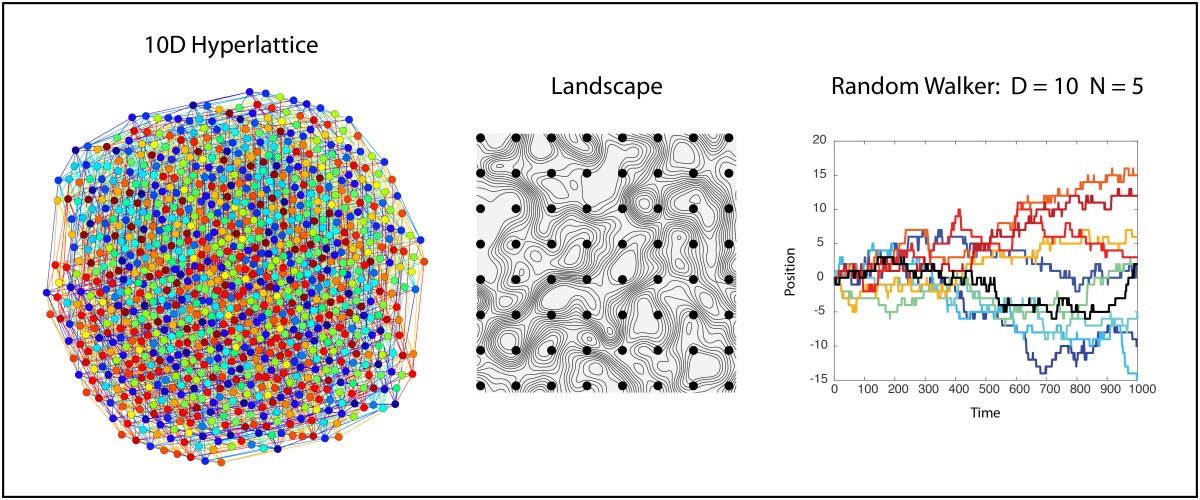
An unconstrained random walk in 10D is just a minimal extension beyond a simple random walk in 1D. Because each dimension is independent, a single random walker takes a random step along any of the 10 dimensions at each iteration so that motion in any one of the 10 dimensions is just a 1D random walk. Therefore, a simple way to visualize this random walk in 10D is simply to plot the walk against each dimension, as in Fig. 3. There is one chance in ten that the walker will take a positive or negative step along any given dimension at each time point.

Fig. 3 A single walker taking random unit steps in 10 dimensions. The position of the walker as a function of time is shown for all ten dimensions.

An alternate visualization of the 10D random walker is shown in Fig. 4 for the same data as Fig. 3. In this case the displacement is color coded, and each column is a different dimension. Time is on the vertical axis (starting at the top and increasing downward). This type of color map can easily be extended to hundreds of dimensions. Each row is a position vector of the single walker in the 10D space

Fig. 4 Same data as in Fig. 3 for a single 10D random walker on a hyperlattice. Distance is color coded. Time is on the vertical axis (increasing downward). Each row is a 10D position vector, and this representation is of a single 10D trajectory.

In the 10D hyperlattice in this section, all lattice sites are accessible at each time point, so there is no constraint preventing the walk from visiting a previously-visited node. There is a possible adjustment that can be made to the walk that prevents it from ever crossing its own path. This is known as a self-avoiding-walk (SAW). In two dimensions, there is a major difference in the geometric and dynamical properties of an ordinary walk and an SAW. However, in dimensions larger than 4, it turns out that there are so many possibilities of where to go (high-dimensional spaces have so much free room) that it is highly unlikely that a random walk will ever cross itself. Therefore, in our 10D hyperlattice we do not need to make the distinction between an ordinary walk and a self-avoiding-walk. However, there are other constraints that can be imposed that mimic how complex systems evolve in time, and these constraints can have important consequences, as we see next.

Random Walk in a Maximally Rough Landscape

In the infinite hyperlattice of the previous section, all lattice sites are the same and are all equally accessible. However, in the study of complex systems, it is common to assign a value to each node in a high-dimensional lattice. This value can be assigned by a potential function, producing a high-dimensional potential landscape over the lattice geometry. Or the value might be the survival fitness of a species, producing a high-dimensional fitness landscape that governs how species compete and evolve. Or the value might be a loss function (an objective function) in a minimization problem from multivariate analysis or machine learning. In all of these cases, the scalar value on the nodes defines a landscape over which a state point executes a walk. The question then becomes, what are the properties of a landscape in high dimensions, and how does it affect a random walker?

As an example, let’s consider a landscape that is completely random point-to-point. There are no correlations in this landscape, making it maximally rough. Then we require that a random walker takes a walk along iso-potentials in this landscape, never increasing and never decreasing its potential. Beginning with our spatial intuition living in 3D space, we might be concerned that such a walker would quickly get confined in some area of the lanscape. Think of a 2D topo map with countour lines drawn on it — If we start at a certain elevation on a mountain side, then if we must walk along directions that maintain our elevation, we stay on a given contour and eventually come back to our starting point after circling the mountain peak — we are trapped! But this intuition informed by our 3D lives is misleading. What happens in our 10D hyperlattice?

To make the example easy to analyze, let’s assume that our potential function is restricted to N discrete values. This means that of the 10 neighbors to a given walker site, on average only 10/N are likely to have the same potential value as the given walker site. This constrains the available sites for the walker, and it converts the uniform hyperlattice into a hyperlattice site percolation problem.

Percolation theory is a fascinating topic in statistical physics. There are many deep concepts that come from asking simple questions about how nodes are connected across a network. The most important aspect of percolation theory is the concept of a percolation threshold. Starting with a complete network that is connected end-to-end, start removing nodes at random. For some critical fraction of nodes removed (on average) there will no longer be a single connected cluster that spans the network. This critical fraction is known as the percolation threshold. Above the percolation threshold, a random walker can get from one part of the network to another. Below the percolation threshold, the random walker is confined to a local cluster.

If a hyperlattice has N discrete values for the landscape potential (or height, or contour) and if a random walker can only move to site that has the same value as the walker’s current value (remains on the level set), then only a fraction of the hyperlattice sites are available to the walker, and the question of whether the walker can find a path the spans the hyperlattice becomes simply a question of how the fraction of available sites relates to the percolation threshold.

The percolation threshold for hyperlattices is well known. For reasonably high dimensions, it is given to good accuracy by

where d is the dimension of the hyperlattice. For a 10D hyperlattice the percolation threshold is pc(10) = 0.0568, or about 6%. Therefore, if more than 6% of the sites of the hyperlattice have the same value as the walker’s current site, then the walker is free to roam about the hyperlattice.

If there are N = 5 discrete values for the potential, then 20% of the sites are available, which is above the percolation threshold, and walkers can go as far as they want. This statement holds true no matter what the starting value is. It might be 5, which means the walker is as high on the landscape as they can get. Or it might be 1, which means the walker is as low on the landscape as they can get. Yet even if they are at the top, if the available site fraction is above the percolation threshold, then the walker can stay on the high mountain ridge, spanning the landscape. The same is true if they start at the bottom of a valley. Therefore, mountain ridges are very common, as are deep valleys, yet they allow full mobility about the geography. On the other hand, a so-called mountain peak would be a 5 surrounded by 4’s or lower. The odds for having this happen in 10D are 0.2*(1-0.8^10) = 0.18. Then the total density of mountain peaks, in a 10D hyperlattice with 5 potential values, is only 18%. Therefore, mountain peaks are rare in 10D, while mountain ridges are common. In even higher dimensions, the percolation threshold decreases roughly inversely with the dimensionality, and mountain peaks become extremely rare and play virtually no part in walks about the landscape.

To illustrate this point, Fig. 5 is the same 10D network that is in Fig. 2, but only the nodes sharing the same value are shown for N = 5, which means that only 20% of the nodes are accessible to a walker who stays only on nodes with the same values. There is a “giant cluster” that remains connected, spanning the original network. If the original network is infinite, then the giant cluster is also infinite but contains a finite fraction of the nodes.

Fig. 5 A 10D cluster that spans the network in Fig. 2 for 1/5 of the nodes sharing the same landscape value. This cluster represents a mountain ridge that spans the space. There are four additional co-existing clusters, each of which separately spans the same 10D space.

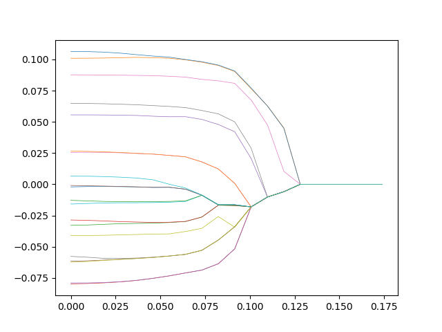
The quantitative details of the random walk can change depending on the proximity of the sub-networks (the clusters, the ridges or the level sets) to the percolation threshold. For instance, a random walker in D =10 with N = 5 is shown in Fig. 6. The diffusion is a bit slower than in the unconstrained walk of Figs. 3 and 4. But the ability to wander about the 10D space is retained.

Fig. 6 A random walker on the level-set cluster of Fig. 5

This is then the general important result: In high-dimensional landscapes, mountain ridges are much more common than mountain peaks. This has profound consequences for the evolution of life, the dynamics of complex systems, and the power of machine learning.

Consequences for Evolution and Machine Learning

When the high-dimensional space is the space of possible mutations on a genome, and when the landscape is a fitness landscape that assigns a survival advantage for one mutation relative to others, then the random walk describes the evolution of a species across generations. The prevalence of ridges, or more generally level sets, in high dimensions has a major consequence for the evolutionary process, because a species can walk along a level set acquiring many possible mutations that have only neutral effects on the survivability of the species. At the same time, the genetic make-up is constantly drifting around in this “neutral network”, allowing the species’ genome to access distant parts of the space. Then, at some point, natural selection may tip the species up a nearby (but rare) peak, and a new equilibrium is attained for the species.

One of the early criticisms of fitness landscapes was the (erroneous) criticism that for a species to move from one fitness peak to another, it would have to go down and cross wide valleys of low fitness to get to another peak. But this was a left-over from thinking in 3D. In high-D, neutral networks are ubiquitous, and a mutation can take a step away from one fitness peak onto one of the neutral networks, which can be sampled by a random walk until the state is near some distant peak. It is no longer necessary to think in terms of high peaks and low valleys of fitness — just random walks. The evolution of extremely complex structures, like ATP synthase, can then be understood as a random walk along networks of nearly-neutral fitness — once our 3D biases are eliminated.

The same arguments hold for many situations in machine learning and especially deep learning. When training a deep neural network, there can be thousands of neural weights that need to be trained through the minimization of a loss function, also known as an objective function. The loss function is the equivalent to a potential, and minimizing the loss function over the thousands of dimensions is the same problem as maximizing the fitness of an evolving species.

At first look, one might think that deep learning is doomed to failure. We have all learned, from the earliest days in calculus, that enough adjustable parameter can fit anything, but the fit is meaningless because it predicts nothing. Deep learning seems to be the worst example of this. How can fitting thousands of adjustable parameters be useful when the dimensionality of the optimization space is orders of magnitude larger than the degrees of freedom of the system being modeled?

The answer comes from the geometry of high dimensions. The prevalence of neutral networks in high dimensions gives lots of chances to escape local minima. In fact, local minima are actually rare in high dimensions, and when they do occur, there is a neutral network nearby onto which they can escape (if the effective temperature of the learning process is set sufficiently high). Therefore, despite the insanely large number of adjustable parameters, general solutions, that are meaningful and predictive, can be found by adding random walks around the objective landscape as a partial strategy in combination with gradient descent.

Given the superficial analogy of deep learning to the human mind, the geometry of random walks in ultra-high dimensions may partially explain our own intelligence and consciousness.

Biblography

S. Gravilet, Fitness Landscapes and the Origins of Species. Princeton University Press, 2004.

M. Kimura, The Neutral Theory of Molecular Evolution. Cambridge University Press, 1968.

YouTube Vlog on A Random Walk in 10 Dimensions

Timelines in the History and Physics of Dynamics (with links to primary texts)

These timelines in the History of Dynamics are organized along the Chapters in Galileo Unbound (Oxford, 2018). The book is about the physics and history of dynamics including classical and quantum mechanics as well as general relativity and nonlinear dynamics (with a detour down evolutionary dynamics and game theory along the way). The first few chapters focus on Galileo, while the following chapters follow his legacy, as theories of motion became more abstract, eventually to encompass the evolution of species within the same theoretical framework as the orbit of photons around black holes.

Galileo: A New Scientist

Galileo Galilei was the first modern scientist, launching a new scientific method that superseded, after one and a half millennia, Aristotle’s physics.  Galileo’s career began with his studies of motion at the University of Pisa that were interrupted by his move to the University of Padua and his telescopic discoveries of mountains on the moon and the moons of Jupiter.  Galileo became the first rock star of science, and he used his fame to promote the ideas of Copernicus and the Sun-centered model of the solar system.  But he pushed too far when he lampooned the Pope.  Ironically, Galileo’s conviction for heresy and his sentence to house arrest for the remainder of his life gave him the free time to finally finish his work on the physics of motion, which he published in Two New Sciences in 1638.

1543 Copernicus dies, publishes posthumously De Revolutionibus

1564    Galileo born

1581    Enters University of Pisa

1585    Leaves Pisa without a degree

1586    Invents hydrostatic balance

1588    Receives lecturship in mathematics at Pisa

1592    Chair of mathematics at Univeristy of Padua

1595    Theory of the tides

1595    Invents military and geometric compass

1596    Le Meccaniche and the principle of horizontal inertia

1600    Bruno Giordano burned at the stake

1601    Death of Tycho Brahe

1609    Galileo constructs his first telescope, makes observations of the moon

1610    Galileo discovers 4 moons of Jupiter, Starry Messenger (Sidereus Nuncius), appointed chief philosopher and mathematician of the Duke of Tuscany, moves to Florence, observes Saturn, Venus goes through phases like the moon

1611    Galileo travels to Rome, inducted into the Lyncean Academy, name “telescope” is first used

1611    Scheiner discovers sunspots

1611    Galileo meets Barberini, a cardinal

1611 Johannes Kepler, Dioptrice

1613    Letters on sunspots published by Lincean Academy in Rome

1614    Galileo denounced from the pulpit

1615    (April) Bellarmine writes an essay against Coperinicus

1615    Galileo investigated by the Inquisition

1615    Writes Letter to Christina, but does not publish it

1615    (December) travels to Rome and stays at Tuscan embassy

1616    (January) Francesco Ingoli publishes essay against Copernicus

1616    (March) Decree against copernicanism

1616    Galileo publishes theory of tides, Galileo meets with Pope Paul V, Copernicus’ book is banned, Galileo warned not to support the Coperinican system, Galileo decides not to reply to Ingoli, Galileo proposes eclipses of Jupter’s moons to determine longitude at sea

1618    Three comets appear, Grassi gives a lecture not hostile to Galileo

1618    Galileo, through Mario Guiducci, publishes scathing attack on Grassi

1619    Jesuit Grassi (Sarsi) publishes attack on Galileo concerning 3 comets

1619    Marina Gamba dies, Galileo legitimizes his son Vinczenzio

1619 Kepler’s Laws, Epitome astronomiae Copernicanae.

1623    Barberini becomes Urban VIII, The Assayer published (response to Grassi)

1624    Galileo visits Rome and Urban VIII

1629    Birth of his grandson Galileo

1630    Death of Johanes Kepler

1632    Publication of the Dialogue Concerning the Two Chief World Systems, Galileo is indicted by the Inquisition (68 years old)

1633    (February) Travels to Rome

1633    Convicted, abjurs, house arrest in Rome, then Siena, then home to Arcetri

1638    Blind, publication of Two New Sciences

1642    Galileo dies (77 years old)

Galileo’s Trajectory

Galileo’s discovery of the law of fall and the parabolic trajectory began with early work on the physics of motion by predecessors like the Oxford Scholars, Tartaglia and the polymath Simon Stevin who dropped lead weights from the leaning tower of Delft three years before Galileo (may have) dropped lead weights from the leaning tower of Pisa.  The story of how Galileo developed his ideas of motion is described in the context of his studies of balls rolling on inclined plane and the surprising accuracy he achieved without access to modern timekeeping.

1583    Galileo Notices isochronism of the pendulum

1588    Receives lecturship in mathematics at Pisa

1589 – 1592  Work on projectile motion in Pisa

1592    Chair of mathematics at Univeristy of Padua

1596    Le Meccaniche and the principle of horizontal inertia

1600    Guidobaldo shares technique of colored ball

1602    Proves isochronism of the pendulum (experimentally)

1604    First experiments on uniformly accelerated motion

1604    Wrote to Scarpi about the law of fall (s ≈ t2)

1607-1608  Identified trajectory as parabolic

1609    Velocity proportional to time

1632    Publication of the Dialogue Concerning the Two Chief World Systems, Galileo is indicted by the Inquisition (68 years old)

1636    Letter to Christina published in Augsburg in Latin and Italian

1638    Blind, publication of Two New Sciences

1641    Invented pendulum clock (in theory)

1642    Dies (77 years old)

On the Shoulders of Giants

Galileo’s parabolic trajectory launched a new approach to physics that was taken up by a new generation of scientists like Isaac Newton, Robert Hooke and Edmund Halley.  The English Newtonian tradition was adopted by ambitious French iconoclasts who championed Newton over their own Descartes.  Chief among these was Pierre Maupertuis, whose principle of least action was developed by Leonhard Euler and Joseph Lagrange into a rigorous new science of dynamics.  Along the way, Maupertuis became embroiled in a famous dispute that entangled the King of Prussia as well as the volatile Voltaire who was mourning the death of his mistress Emilie du Chatelet, the lone female French physicist of the eighteenth century.

1644    Descartes’ vortex theory of gravitation

1662    Fermat’s principle

1669 – 1690    Huygens expands on Descartes’ vortex theory

1687 Newton’s Principia

1698    Maupertuis born

1729    Maupertuis entered University in Basel.  Studied under Johann Bernoulli

1736    Euler publishes Mechanica sive motus scientia analytice exposita

1737   Maupertuis report on expedition to Lapland.  Earth is oblate.  Attacks Cassini.

1744    Maupertuis Principle of Least Action.  Euler Principle of Least Action.

1745    Maupertuis becomes president of Berlin Academy.  Paris Academy cancels his membership after a campaign against him by Cassini.

1746    Maupertuis principle of Least Action for mass

1751    Samuel König disputes Maupertuis’ priority

1756    Cassini dies.  Maupertuis reinstated in the French Academy

1759    Maupertuis dies

1759    du Chatelet’s French translation of Newton’s Principia published posthumously

1760    Euler 3-body problem (two fixed centers and coplanar third body)

1760-1761 Lagrange, Variational calculus (J. L. Lagrange, “Essai d’une nouvelle méthod pour dEeterminer les maxima et lest minima des formules intégrales indéfinies,” Miscellanea Teurinensia, (1760-1761))

1762    Beginning of the reign of Catherine the Great of Russia

1763    Euler colinear 3-body problem

1765    Euler publishes Theoria motus corporum solidorum on rotational mechanics

1766    Euler returns to St. Petersburg

1766    Lagrange arrives in Berlin

1772    Lagrange equilateral 3-body problem, Essai sur le problème des trois corps, 1772, Oeuvres tome 6

1775    Beginning of the American War of Independence

1776    Adam Smith Wealth of Nations

1781    William Herschel discovers Uranus

1783    Euler dies in St. Petersburg

1787    United States Constitution written

1787    Lagrange moves from Berlin to Paris

1788    Lagrange, Méchanique analytique

1789    Beginning of the French Revolution

1799    Pierre-Simon Laplace Mécanique Céleste (1799-1825)

Geometry on My Mind

This history of modern geometry focuses on the topics that provided the foundation for the new visualization of physics.  It begins with Carl Gauss and Bernhard Riemann, who redefined geometry and identified the importance of curvature for physics.  Vector spaces, developed by Hermann Grassmann, Giuseppe Peano and David Hilbert, are examples of the kinds of abstract new spaces that are so important for modern physics, such as Hilbert space for quantum mechanics.  Fractal geometry developed by Felix Hausdorff later provided the geometric language needed to solve problems in chaos theory.

1629    Fermat described higher-dim loci

1637    Descarte’s Geometry

1649    van Schooten’s commentary on Descartes Geometry

1694    Leibniz uses word “coordinate” in its modern usage

1697    Johann Bernoulli shortest distance between two points on convex surface

1732    Euler geodesic equations for implicit surfaces

1748    Euler defines modern usage of function

1801    Gauss calculates orbit of Ceres

1807    Fourier analysis (published in 1822(

1807    Gauss arrives in Göttingen

1827    Karl Gauss establishes differential geometry of curved surfaces, Disquisitiones generales circa superficies curvas

1830    Bolyai and Lobachevsky publish on hyperbolic geometry

1834    Jacobi n-fold integrals and volumes of n-dim spheres

1836    Liouville-Sturm theorem

1838    Liouville’s theorem

1841    Jacobi determinants

1843    Arthur Cayley systems of n-variables

1843    Hamilton discovers quaternions

1844    Hermann Grassman n-dim vector spaces, Die Lineale Ausdehnungslehr

1846    Julius Plücker System der Geometrie des Raumes in neuer analytischer Behandlungsweise

1848 Jacobi Vorlesungen über Dynamik

1848    “Vector” coined by Hamilton

1854    Riemann’s habilitation lecture

1861    Riemann n-dim solution of heat conduction

1868    Publication of Riemann’s Habilitation

1869    Christoffel and Lipschitz work on multiple dimensional analysis

1871    Betti refers to the n-ply of numbers as a “space”.

1871    Klein publishes on non-euclidean geometry

1872 Boltzmann distribution

1872    Jordan Essay on the geometry of n-dimensions

1872    Felix Klein’s “Erlangen Programme”

1872    Weierstrass’ Monster

1872    Dedekind cut

1872    Cantor paper on irrational numbers

1872    Cantor meets Dedekind

1872 Lipschitz derives mechanical motion as a geodesic on a manifold

1874    Cantor beginning of set theory

1877    Cantor one-to-one correspondence between the line and n-dimensional space

1881    Gibbs codifies vector analysis

1883    Cantor set and staircase Grundlagen einer allgemeinen Mannigfaltigkeitslehre

1884    Abbott publishes Flatland

1887    Peano vector methods in differential geometry

1890    Peano space filling curve

1891    Hilbert space filling curve

1887    Darboux vol. 2 treats dynamics as a point in d-dimensional space.  Applies concepts of geodesics for trajectories.

1898    Ricci-Curbastro Lesons on the Theory of Surfaces

1902    Lebesgue integral

1904    Hilbert studies integral equations

1904    von Koch snowflake

1906    Frechet thesis on square summable sequences as infinite dimensional space

1908    Schmidt Geometry in a Function Space

1910    Brouwer proof of dimensional invariance

1913    Hilbert space named by Riesz

1914    Hilbert space used by Hausdorff

1915    Sierpinski fractal triangle

1918    Hausdorff non-integer dimensions

1918    Weyl’s book Space, Time, Matter

1918    Fatou and Julia fractals

1920    Banach space

1927    von Neumann axiomatic form of Hilbert Space

1935    Frechet full form of Hilbert Space

1967    Mandelbrot coast of Britain

1982    Mandelbrot’s book The Fractal Geometry of Nature

The Tangled Tale of Phase Space

Phase space is the central visualization tool used today to study complex systems.  The chapter describes the origins of phase space with the work of Joseph Liouville and Carl Jacobi that was later refined by Ludwig Boltzmann and Rudolf Clausius in their attempts to define and explain the subtle concept of entropy.  The turning point in the history of phase space was when Henri Poincaré used phase space to solve the three-body problem, uncovering chaotic behavior in his quest to answer questions on the stability of the solar system.  Phase space was established as the central paradigm of statistical mechanics by JW Gibbs and Paul Ehrenfest.

1804    Jacobi born (1904 – 1851) in Potsdam

1804    Napoleon I Emperor of France

1806    William Rowan Hamilton born (1805 – 1865)

1807    Thomas Young describes “Energy” in his Course on Natural Philosophy (Vol. 1 and Vol. 2)

1808    Bethoven performs his Fifth Symphony

1809    Joseph Liouville born (1809 – 1882)

1821    Hermann Ludwig Ferdinand von Helmholtz born (1821 – 1894)

1824    Carnot published Reflections on the Motive Power of Fire

1834    Jacobi n-fold integrals and volumes of n-dim spheres

1834-1835       Hamilton publishes his principle (1834, 1835).

1836    Liouville-Sturm theorem

1837    Queen Victoria begins her reign as Queen of England

1838    Liouville develops his theorem on products of n differentials satisfying certain first-order differential equations.  This becomes the classic reference to Liouville’s Theorem.

1847    Helmholtz  Conservation of Energy (force)

1849    Thomson makes first use of “Energy” (From reading Thomas Young’s lecture notes)

1850    Clausius establishes First law of Thermodynamics: Internal energy. Second law:  Heat cannot flow unaided from cold to hot.  Not explicitly stated as first and second laws

1851    Thomson names Clausius’ First and Second laws of Thermodynamics

1852    Thomson describes general dissipation of the universe (“energy” used in title)

1854    Thomson defined absolute temperature.  First mathematical statement of 2nd law.  Restricted to reversible processes

1854    Clausius stated Second Law of Thermodynamics as inequality

1857    Clausius constructs kinetic theory, Mean molecular speeds

1858    Clausius defines mean free path, Molecules have finite size. Clausius assumed that all molecules had the same speed

1860    Maxwell publishes first paper on kinetic theory. Distribution of speeds. Derivation of gas transport properties

1865    Loschmidt size of molecules

1865    Clausius names entropy

1868    Boltzmann adds (Boltzmann) factor to Maxwell distribution

1872    Boltzmann transport equation and H-theorem

1876    Loschmidt reversibility paradox

1877    Boltzmann  S = k logW

1890    Poincare: Recurrence Theorem. Recurrence paradox with Second Law (1893)

1896    Zermelo criticizes Boltzmann

1896    Boltzmann posits direction of time to save his H-theorem

1898    Boltzmann Vorlesungen über Gas Theorie

1905    Boltzmann kinetic theory of matter in Encyklopädie der mathematischen Wissenschaften

1906    Boltzmann dies

1910    Paul Hertz uses “Phase Space” (Phasenraum)

1911    Ehrenfest’s article in Encyklopädie der mathematischen Wissenschaften

1913    A. Rosenthal writes the first paper using the phrase “phasenraum”, combining the work of Boltzmann and Poincaré. “Beweis der Unmöglichkeit ergodischer Gassysteme” (Ann. D. Physik, 42, 796 (1913)

1913    Plancheral, “Beweis der Unmöglichkeit ergodischer mechanischer Systeme” (Ann. D. Physik, 42, 1061 (1913).  Also uses “Phasenraum”.

The Lens of Gravity

Gravity provided the backdrop for one of the most important paradigm shifts in the history of physics.  Prior to Albert Einstein’s general theory of relativity, trajectories were paths described by geometry.  After the theory of general relativity, trajectories are paths caused by geometry.  This chapter explains how Einstein arrived at his theory of gravity, relying on the space-time geometry of Hermann Minkowski, whose work he had originally harshly criticized.  The confirmation of Einstein’s theory was one of the dramatic high points in 20th century history of physics when Arthur Eddington journeyed to an island off the coast of Africa to observe stellar deflections during a solar eclipse.  If Galileo was the first rock star of physics, then Einstein was the first worldwide rock star of science.

1697    Johann Bernoulli was first to find solution to shortest path between two points on a curved surface (1697).

1728    Euler found the geodesic equation.

1783    The pair 40 Eridani B/C was discovered by William Herschel on 31 January

1783    John Michell explains infalling object would travel faster than speed of light

1796    Laplace describes “dark stars” in Exposition du system du Monde

1827    The first orbit of a binary star computed by Félix Savary for the orbit of Xi Ursae Majoris.

1827    Gauss curvature Theoriem Egregum

1844    Bessel notices periodic displacement of Sirius with period of half a century

1844    The name “geodesic line” is attributed to Liouville.

1845    Buys Ballot used musicians with absolute pitch for the first experimental verification of the Doppler effect

1854    Riemann’s habilitationsschrift

1862    Discovery of Sirius B (a white dwarf)

1868    Darboux suggested motions in n-dimensions

1872    Lipshitz first to apply Riemannian geometry to the principle of least action.

1895    Hilbert arrives in Göttingen

1902    Minkowski arrives in Göttingen

1905    Einstein’s miracle year

1906    Poincaré describes Lorentz transformations as rotations in 4D

1907    Einstein has “happiest thought” in November

1907    Einstein’s relativity review in Jahrbuch

1908    Minkowski’s Space and Time lecture

1908    Einstein appointed to unpaid position at University of Bern

1909    Minkowski dies

1909    Einstein appointed associate professor of theoretical physics at U of Zürich

1910    40 Eridani B was discobered to be of spectral type A (white dwarf)

1910    Size and mass of Sirius B determined (heavy and small)

1911    Laue publishes first textbook on relativity theory

1911    Einstein accepts position at Prague

1911    Einstein goes to the limits of special relativity applied to gravitational fields

1912    Einstein’s two papers establish a scalar field theory of gravitation

1912    Einstein moves from Prague to ETH in Zürich in fall.  Begins collaboration with Grossmann.

1913    Einstein EG paper

1914    Adams publishes spectrum of 40 Eridani B

1915    Sirius B determined to be also a low-luminosity type A white dwarf

1915    Einstein Completes paper

1916    Density of 40 Eridani B by Ernst Öpik

1916    Schwarzschild paper

1916 Einstein’s publishes theory of gravitational waves

1919    Eddington expedition to Principe

1920    Eddington paper on deflection of light by the sun

1922    Willem Luyten coins phrase “white dwarf”

1924    Eddington found a set of coordinates that eliminated the singularity at the Schwarzschild radius

1926    R. H. Fowler publishes paper on degenerate matter and composition of white dwarfs

1931    Chandrasekhar calculated the limit for collapse to white dwarf stars at 1.4MS

1933    Georges Lemaitre states the coordinate singularity was an artefact

1934    Walter Baade and Fritz Zwicky proposed the existence of the neutron star only a year after the discovery of the neutron by Sir James Chadwick.

1939    Oppenheimer and Snyder showed ultimate collapse of a 3MS  “frozen star”

1958    David Finkelstein paper

1965    Antony Hewish and Samuel Okoye discovered “an unusual source of high radio brightness temperature in the Crab Nebula”. This source turned out to be the Crab Nebula neutron star that resulted from the great supernova of 1054.

1967    Jocelyn Bell and Antony Hewish discovered regular radio pulses from CP 1919. This pulsar was later interpreted as an isolated, rotating neutron star.

1967    Wheeler’s “black hole” talk

1974    Joseph Taylor and Russell Hulse discovered the first binary pulsar, PSR B1913+16, which consists of two neutron stars (one seen as a pulsar) orbiting around their center of mass.

2015    LIGO detects gravitational waves on Sept. 14 from the merger of two black holes

2017    LIGO detects the merger of two neutron stars

On the Quantum Footpath

The concept of the trajectory of a quantum particle almost vanished in the battle between Werner Heisenberg’s matrix mechanics and Erwin Schrödinger’s wave mechanics.  It took Niels Bohr and his complementarity principle of wave-particle duality to cede back some reality to quantum trajectories.  However, Schrödinger and Einstein were not convinced and conceived of quantum entanglement to refute the growing acceptance of the Copenhagen Interpretation of quantum physics.  Schrödinger’s cat was meant to be an absurdity, but ironically it has become a central paradigm of practical quantum computers.  Quantum trajectories took on new meaning when Richard Feynman constructed quantum theory based on the principle of least action, inventing his famous Feynman Diagrams to help explain quantum electrodynamics.

1885    Balmer Theory

1897    J. J. Thomson discovered the electron

1904    Thomson plum pudding model of the atom

1911    Bohr PhD thesis filed. Studies on the electron theory of metals.  Visited England.

1911    Rutherford nuclear model

1911    First Solvay conference

1911    “ultraviolet catastrophe” coined by Ehrenfest

1913    Bohr combined Rutherford’s nuclear atom with Planck’s quantum hypothesis: 1913 Bohr model

1913    Ehrenfest adiabatic hypothesis

1914-1916       Bohr at Manchester with Rutherford

1916    Bohr appointed Chair of Theoretical Physics at University of Copenhagen: a position that was made just for him

1916    Schwarzschild and Epstein introduce action-angle coordinates into quantum theory

1920    Heisenberg enters University of Munich to obtain his doctorate

1920    Bohr’s Correspondence principle: Classical physics for large quantum numbers

1921    Bohr Founded Institute of Theoretical Physics (Copenhagen)

1922-1923       Heisenberg studies with Born, Franck and Hilbert at Göttingen while Sommerfeld is in the US on sabbatical.

1923    Heisenberg Doctorate.  The exam does not go well.  Unable to derive the resolving power of a microscope in response to question by Wien.  Becomes Born’s assistant at Göttingen.

1924    Heisenberg visits Niels Bohr in Copenhagen (and met Einstein?)

1924    Heisenberg Habilitation at Göttingen on anomalous Zeeman

1924 – 1925    Heisenberg worked with Bohr in Copenhagen, returned summer of 1925 to Göttiingen

1924    Pauli exclusion principle and state occupancy

1924    de Broglie hypothesis extended wave-particle duality to matter

1924    Bohr Predicted Halfnium (72)

1924    Kronig’s proposal for electron self spin

1924    Bose (Einstein)

1925    Heisenberg paper on quantum mechanics

1925    Dirac, reading proof from Heisenberg, recognized the analogy of noncommutativity with Poisson brackets and the correspondence with Hamiltonian mechanics.

1925    Uhlenbeck and Goudschmidt: spin

1926    Born, Heisenberg, Kramers: virtual oscillators at transition frequencies: Matrix mechanics (alternative to Bohr-Kramers-Slater 1924 model of orbits).  Heisenberg was Born’s student at Göttingen.

1926    Schrödinger wave mechanics

1927    de Broglie hypotehsis confirmed by Davisson and Germer

1927    Complementarity by Bohr: wave-particle duality “Evidence obtained under different experimental conditions cannot be comprehended within a single picture, but must be regarded as complementary in the sense that only the totality of the phenomena exhausts the possible information about the objects.

1927    Heisenberg uncertainty principle (Heisenberg was in Copenhagen 1926 – 1927)

1927    Solvay Conference in Brussels

1928    Heisenberg to University of Leipzig

1928    Dirac relativistic QM equation

1929    de Broglie Nobel Prize

1930    Solvay Conference

1932    Heisenberg Nobel Prize

1932    von Neumann operator algebra

1933    Dirac Lagrangian form of QM (basis of Feynman path integral)

1933    Schrödinger and Dirac Nobel Prize

1935    Einstein, Poldolsky and Rosen EPR paper

1935 Bohr’s response to Einsteins “EPR” paradox

1935    Schrodinger’s cat

1939    Feynman graduates from MIT

1941    Heisenberg (head of German atomic project) visits Bohr in Copenhagen

1942    Feynman PhD at Princeton, “The Principle of Least Action in Quantum Mechanics

1942 – 1945    Manhattan Project, Bethe-Feynman equation for fission yield

1943    Bohr escapes to Sweden in a fishing boat.  Went on to England secretly.

1945    Pauli Nobel Prize

1945    Death of Feynman’s wife Arline (married 4 years)

1945    Fall, Feynman arrives at Cornell ahead of Hans Bethe

1947    Shelter Island conference: Lamb Shift, did Kramer’s give a talk suggesting that infinities could be subtracted?

1947    Fall, Dyson arrives at Cornell

1948    Pocono Manor, Pennsylvania, troubled unveiling of path integral formulation and Feynman diagrams, Schwinger’s master presentation

1948    Feynman and Dirac. Summer drive across the US with Dyson

1949    Dyson joins IAS as a postdoc, trains a cohort of theorists in Feynman’s technique

1949    Karplus and Kroll first g-factor calculation

1950    Feynman moves to Cal Tech

1965    Schwinger, Tomonaga and Feynman Nobel Prize

1967    Hans Bethe Nobel Prize

From Butterflies to Hurricanes

Half a century after Poincaré first glimpsed chaos in the three-body problem, the great Russian mathematician Andrey Kolmogorov presented a sketch of a theorem that could prove that orbits are stable.  In the hands of Vladimir Arnold and Jürgen Moser, this became the KAM theory of Hamiltonian chaos.  This chapter shows how KAM theory fed into topology in the hands of Stephen Smale and helped launch the new field of chaos theory.  Edward Lorenz discovered chaos in numerical models of atmospheric weather and discovered the eponymous strange attractor.  Mathematical aspects of chaos were further developed by Mitchell Feigenbaum studying bifurcations in the logistic map that describes population dynamics.

1760    Euler 3-body problem (two fixed centers and coplanar third body)

1763    Euler colinear 3-body problem

1772    Lagrange equilateral 3-body problem

1881-1886       Poincare memoires “Sur les courbes de ́finies par une equation differentielle”

1890    Poincare “Sur le probleme des trois corps et les equations de la dynamique”. First-return map, Poincare recurrence theorem, stable and unstable manifolds

1892 – 1899    Poincare New Methods in Celestial Mechanics

1892    Lyapunov The General Problem of the Stability of Motion

1899    Poincare homoclinic trajectory

1913    Birkhoff proves Poincaré’s last geometric theorem, a special case of the three-body problem.

1927    van der Pol and van der Mark

1937    Coarse systems, Andronov and Pontryagin

1938    Morse theory

1942    Hopf bifurcation

1945    Cartwright and Littlewood study the van der Pol equation (Radar during WWII)

1954    Kolmogorov A. N., On conservation of conditionally periodic motions for a small change in Hamilton’s function.

1960    Lorenz: 12 equations

1962    Moser On Invariant Curves of Area-Preserving Mappings of an Annulus.

1963    Arnold Small denominators and problems of the stability of motion in classical and celestial mechanics

1963    Lorenz: 3 equations

1964    Arnold diffusion

1965    Smale’s horseshoe

1969    Chirikov standard map

1971    Ruelle-Takens (Ruelle coins phrase “strange attractor”)

1972    “Butterfly Effect” given for Lorenz’ talk (by Philip Merilees)

1975    Gollub-Swinney observe route to turbulence along lines of Ruelle

1975    Yorke coins “chaos theory”

1976    Robert May writes review article of the logistic map

1977    New York conference on bifurcation theory

1987    James Gleick Chaos: Making a New Science

Darwin in the Clockworks

The preceding timelines related to the central role played by families of trajectories phase space to explain the time evolution of complex systems.  These ideas are extended to explore the history and development of the theory of natural evolution by Charles Darwin.  Darwin had many influences, including ideas from Thomas Malthus in the context of economic dynamics.  After Darwin, the ideas of evolution matured to encompass broad topics in evolutionary dynamics and the emergence of the idea of fitness landscapes and game theory driving the origin of new species.  The rise of genetics with Gregor Mendel supplied a firm foundation for molecular evolution, leading to the moleculer clock of Linus Pauling and the replicator dynamics of Richard Dawkins.

1202    Fibonacci

1766    Thomas Robert Malthus born

1776    Adam Smith The Wealth of Nations

1798    Malthus “An Essay on the Principle of Population

1817    Ricardo Principles of Political Economy and Taxation

1838    Cournot early equilibrium theory in duopoly

1848    John Stuart Mill

1848    Karl Marx Communist Manifesto

1859    Darwin Origin of Species

1867    Karl Marx Das Kapital

1871    Darwin Descent of Man, and Selection in Relation to Sex

1871    Jevons Theory of Political Economy

1871    Menger Principles of Economics

1874    Walrus Éléments d’économie politique pure, or Elements of Pure Economics (1954)

1890    Marshall Principles of Economics

1908    Hardy constant genetic variance

1910    Brouwer fixed point theorem

1910    Alfred J. Lotka autocatylitic chemical reactions

1913    Zermelo determinancy in chess

1922    Fisher dominance ratio

1922    Fisher mutations

1925    Lotka predator-prey in biomathematics

1926    Vita Volterra published same equations independently

1927    JBS Haldane (1892—1964) mutations

1928    von Neumann proves the minimax theorem

1930    Fisher ratio of sexes

1932    Wright Adaptive Landscape

1932    Haldane The Causes of Evolution

1933    Kolmogorov Foundations of the Theory of Probability

1934    Rudolph Carnap The Logical Syntax of Language

1936    John Maynard Keynes, The General Theory of Employment, Interest and Money

1936    Kolmogorov generalized predator-prey systems

1938    Borel symmetric payoff matrix

1942    Sewall Wright    Statistical Genetics and Evolution

1943    McCulloch and Pitts A Logical Calculus of Ideas Immanent in Nervous Activity

1944    von Neumann and Morgenstern Theory of Games and Economic Behavior

1950    Prisoner’s Dilemma simulated at Rand Corportation

1950    John Nash Equilibrium points in n-person games and The Bargaining Problem

1951    John Nash Non-cooperative Games

1952    McKinsey Introduction to the Theory of Games (first textbook)

1953    John Nash Two-Person Cooperative Games

1953    Watson and Crick DNA

1955    Braithwaite’s Theory of Games as a Tool for the Moral Philosopher

1961    Lewontin Evolution and the Theory of Games

1962    Patrick Moran The Statistical Processes of Evolutionary Theory

1962    Linus Pauling molecular clock

1968    Motoo Kimura  neutral theory of molecular evolution

1972    Maynard Smith introduces the evolutionary stable solution (ESS)

1972    Gould and Eldridge Punctuated equilibrium

1973    Maynard Smith and Price The Logic of Animal Conflict

1973    Black Scholes

1977    Eigen and Schuster The Hypercycle

1978    Replicator equation (Taylor and Jonker)

1982    Hopfield network

1982    John Maynard Smith Evolution and the Theory of Games

1984    R. Axelrod The Evolution of Cooperation

The Measure of Life

This final topic extends the ideas of dynamics into abstract spaces of high dimension to encompass the idea of a trajectory of life.  Health and disease become dynamical systems defined by all the proteins and nucleic acids that comprise the physical self.  Concepts from network theory, autonomous oscillators and synchronization contribute to this viewpoint.  Healthy trajectories are like stable limit cycles in phase space, but disease can knock the system trajectory into dangerous regions of health space, as doctors turn to new developments in personalized medicine try to return the individual to a healthy path.  This is the ultimate generalization of Galileo’s simple parabolic trajectory.

1642    Galileo dies

1656    Huygens invents pendulum clock

1665    Huygens observes “odd kind of sympathy” in synchronized clocks

1673    Huygens publishes Horologium Oscillatorium sive de motu pendulorum

1736    Euler Seven Bridges of Königsberg

1845    Kirchhoff’s circuit laws

1852    Guthrie four color problem

1857    Cayley trees

1858    Hamiltonian cycles

1887    Cajal neural staining microscopy

1913    Michaelis Menten dynamics of enzymes

1924    Berger, Hans: neural oscillations (Berger invented the EEG)

1926    van der Pol dimensioness form of equation

1927    van der Pol periodic forcing

1943    McCulloch and Pits mathematical model of neural nets

1948    Wiener cybernetics

1952    Hodgkin and Huxley action potential model

1952    Turing instability model

1956    Sutherland cyclic AMP

1957    Broadbent and Hammersley bond percolation

1958    Rosenblatt perceptron

1959    Erdös and Renyi random graphs

1962    Cohen EGF discovered

1965    Sebeok coined zoosemiotics

1966    Mesarovich systems biology

1967    Winfree biological rythms and coupled oscillators

1969    Glass Moire patterns in perception

1970    Rodbell G-protein

1971    phrase “strange attractor” coined (Ruelle)

1972    phrase “signal transduction” coined (Rensing)

1975    phrase “chaos theory” coined (Yorke)

1975    Werbos backpropagation

1975    Kuramoto transition

1976    Robert May logistic map

1977    Mackey-Glass equation and dynamical disease

1982    Hopfield network

1990    Strogatz and Murillo pulse-coupled oscillators

1997    Tomita systems biology of a cell

1998    Strogatz and Watts Small World network

1999    Barabasi Scale Free networks

2000    Sequencing of the human genome


Read all the stories behind the history of modern dynamics, in Galileo Unbound from Oxford Press:


References

Second Edition of Introduction to Modern Dynamics (Chaos, Networks, Space and Time)

The second edition of Introduction to Modern Dynamics: Chaos, Networks, Space and Time is available from Oxford University Press and Amazon.

Most physics majors will use modern dynamics in their careers: nonlinearity, chaos, network theory, econophysics, game theory, neural nets, geodesic geometry, among many others.

The first edition of Introduction to Modern Dynamics (IMD) was an upper-division junior-level mechanics textbook at the level of Thornton and Marion (Classical Dynamics of Particles and Systems) and Taylor (Classical Mechanics).  IMD helped lead an emerging trend in physics education to update the undergraduate physics curriculum.  Conventional junior-level mechanics courses emphasized Lagrangian and Hamiltonian physics, but notably missing from the classic subjects are modern dynamics topics that most physics majors will use in their careers: nonlinearity, chaos, network theory, econophysics, game theory, neural nets, geodesic geometry, among many others.  These are the topics at the forefront of physics that drive high-tech businesses and start-ups, which is where more than half of all physicists work. IMD introduced these modern topics to junior-level physics majors in an accessible form that allowed them to master the fundamentals to prepare them for the modern world.

The second edition (IMD2) continues that trend by expanding the chapters to include additional material and topics.  It rearranges several of the introductory chapters for improved logical flow and expands them to include key conventional topics that were missing in the first edition (e.g., Lagrange undetermined multipliers and expanded examples of Lagrangian applications).  It is also an opportunity to correct several typographical errors and other errata that students have identified over the past several years.  The second edition also has expanded homework problems.

The goal of IMD2 is to strengthen the sections on conventional topics (that students need to master to take their GREs) to make IMD2 attractive as a mainstream physics textbook for broader adoption at the junior level, while continuing the program of updating the topics and approaches that are relevant for the roles that physicists play in the 21st century.

(New Chapters and Sections highlighted in red.)

New Features in Second Edition:

Second Edition Chapters and Sections

Part 1 Geometric Mechanics

• Expanded development of Lagrangian dynamics

• Lagrange multipliers

• More examples of applications

• Connection to statistical mechanics through the virial theorem

• Greater emphasis on action-angle variables

• The key role of adiabatic invariants

Part 1 Geometric Mechanics

Chapter 1 Physics and Geometry

1.1 State space and dynamical flows

1.2 Coordinate representations

1.3 Coordinate transformation

1.4 Uniformly rotating frames

1.5 Rigid-body motion

Chapter 2 Lagrangian Mechanics

2.1 Calculus of variations

2.2 Lagrangian applications

2.3 Lagrange’s undetermined multipliers

2.4 Conservation laws

2.5 Central force motion

2.6 Virial Theorem

Chapter 3 Hamiltonian Dynamics and Phase Space

3.1 The Hamiltonian function

3.2 Phase space

3.3 Integrable systems and action–angle variables

3.4 Adiabatic invariants

Part 2 Nonlinear Dynamics

• New section on non-autonomous dynamics

• Entire new chapter devoted to Hamiltonian mechanics

• Added importance to Chirikov standard map

• The important KAM theory of “constrained chaos” and solar system stability

• Degeneracy in Hamiltonian chaos

• A short overview of quantum chaos

• Rational resonances and the relation to KAM theory

• Synchronized chaos

Part 2 Nonlinear Dynamics

Chapter 4 Nonlinear Dynamics and Chaos

4.1 One-variable dynamical systems

4.2 Two-variable dynamical systems

4.3 Limit cycles

4.4 Discrete iterative maps

4.5 Three-dimensional state space and chaos

4.6 Non-autonomous (driven) flows

4.7 Fractals and strange attractors

Chapter 5 Hamiltonian Chaos

5.1 Perturbed Hamiltonian systems

5.2 Nonintegrable Hamiltonian systems

5.3 The Chirikov Standard Map

5.4 KAM Theory

5.5 Degeneracy and the web map

5.6 Quantum chaos

Chapter 6 Coupled Oscillators and Synchronization

6.1 Coupled linear oscillators

6.2 Simple models of synchronization

6.3 Rational resonances

6.4 External synchronization

6.5 Synchronization of Chaos

Part 3 Complex Systems

• New emphasis on diffusion on networks

• Epidemic growth on networks

• A new section of game theory in the context of evolutionary dynamics

• A new section on general equilibrium theory in economics

Part 3 Complex Systems

Chapter 7 Network Dynamics

7.1 Network structures

7.2 Random network topologies

7.3 Synchronization on networks

7.4 Diffusion on networks

7.5 Epidemics on networks

Chapter 8 Evolutionary Dynamics

81 Population dynamics

8.2 Virus infection and immune deficiency

8.3 Replicator Dynamics

8.4 Quasi-species

8.5 Game theory and evolutionary stable solutions

Chapter 9 Neurodynamics and Neural Networks

9.1 Neuron structure and function

9.2 Neuron dynamics

9.3 Network nodes: artificial neurons

9.4 Neural network architectures

9.5 Hopfield neural network

9.6 Content-addressable (associative) memory

Chapter 10 Economic Dynamics

10.1 Microeconomics and equilibrium

10.2 Macroeconomics

10.3 Business cycles

10.4 Random walks and stock prices (optional)

Part 4 Relativity and Space–Time

• Relativistic trajectories

• Gravitational waves

Part 4 Relativity and Space–Time

Chapter 11 Metric Spaces and Geodesic Motion

11.1 Manifolds and metric tensors

11.2 Derivative of a tensor

11.3 Geodesic curves in configuration space

11.4 Geodesic motion

Chapter 12 Relativistic Dynamics

12.1 The special theory

12.2 Lorentz transformations

12.3 Metric structure of Minkowski space

12.4 Relativistic trajectories

12.5 Relativistic dynamics

12.6 Linearly accelerating frames (relativistic)

Chapter 13 The General Theory of Relativity and Gravitation

13.1 Riemann curvature tensor

13.2 The Newtonian correspondence

13.3 Einstein’s field equations

13.4 Schwarzschild space–time

13.5 Kinematic consequences of gravity

13.6 The deflection of light by gravity

13.7 The precession of Mercury’s perihelion

13.8 Orbits near a black hole

13.9 Gravitational waves

Synopsis of 2nd Ed. Chapters

Chapter 1. Physics and Geometry (Sample Chapter)

This chapter has been rearranged relative to the 1st edition to provide a more logical flow of the overarching concepts of geometric mechanics that guide the subsequent chapters.  The central role of coordinate transformations is strengthened, as is the material on rigid-body motion with expanded examples.

Chapter 2. Lagrangian Mechanics (Sample Chapter)

Much of the structure and material is retained from the 1st edition while adding two important sections.  The section on applications of Lagrangian mechanics adds many direct examples of the use of Lagrange’s equations of motion.  An additional new section covers the important topic of Lagrange’s undetermined multipliers

Chapter 3. Hamiltonian Dynamics and Phase Space (Sample Chapter)

The importance of Hamiltonian systems and dynamics merits a stand-alone chapter.  The topics from the 1st edition are expanded in this new chapter, including a new section on adiabatic invariants that plays an important role in the development of quantum theory.  Some topics are de-emphasized from the 1st edition, such as general canonical transformations and the symplectic structure of phase space, although the specific transformation to action-angle coordinates is retained and amplified.

Chapter 4. Nonlinear Dynamics and Chaos

The first part of this chapter is retained from the 1st edition with numerous minor corrections and updates of figures.  The second part of the IMD 1st edition, treating Hamiltonian chaos, will be expanded into the new Chapter 5.

Chapter 5. Hamiltonian Chaos

This new stand-alone chapter expands on the last half of Chapter 3 of the IMD 1st edition.  The physical character of Hamiltonian chaos is substantially distinct from dissipative chaos that it deserves its own chapter.  It is also a central topic of interest for complex systems that are either conservative or that have integral invariants, such as our N-body solar system that played such an important role in the history of chaos theory beginning with Poincaré.  The new chapter highlights Poincaré’s homoclinic tangle, illustrated by the Chirikov Standard Map.  The Standard Map is an excellent introduction to KAM theory, which is one of the crowning achievements of the theory of dynamical systems by Komogorov, Arnold and Moser, connecting to deeper aspects of synchronization and rational resonances that drive the structure of systems as diverse as the rotation of the Moon and the rings of Saturn.  This is also a perfect lead-in to the next chapter on synchronization.  An optional section at the end of this chapter briefly discusses quantum chaos to show how Hamiltonian chaos can be extended into the quantum regime.

Chapter 6. Synchronization

This is an updated version of the IMD 1st ed. chapter.  It has a reduced initial section on coupled linear oscillators, retaining the key ideas about linear eigenmodes but removing some irrelevant details in the 1st edition.  A new section is added that defines and emphasizes the importance of quasi-periodicity.  A new section on the synchronization of chaotic oscillators is added.

Chapter 7. Network Dynamics

This chapter rearranges the structure of the chapter from the 1st edition, moving synchronization on networks earlier to connect from the previous chapter.  The section on diffusion and epidemics is moved to the back of the chapter and expanded in the 2nd edition into two separate sections on these topics, adding new material on discrete matrix approaches to continuous dynamics.

Chapter 8. Neurodynamics and Neural Networks

This chapter is retained from the 1st edition with numerous minor corrections and updates of figures.

Chapter 9. Evolutionary Dynamics

Two new sections are added to this chapter.  A section on game theory and evolutionary stable solutions introduces core concepts of evolutionary dynamics that merge well with the other topics of the chapter such as the pay-off matrix and replicator dynamics.  A new section on nearly neutral networks introduces new types of behavior that occur in high-dimensional spaces which are counter intuitive but important for understanding evolutionary drift.

Chapter 10.  Economic Dynamics

This chapter will be significantly updated relative to the 1st edition.  Most of the sections will be rewritten with improved examples and figures.  Three new sections will be added.  The 1st edition section on consumer market competition will be split into two new sections describing the Cournot duopoly and Pareto optimality in one section, and Walras’ Law and general equilibrium theory in another section.  The concept of the Pareto frontier in economics is becoming an important part of biophysical approaches to population dynamics.  In addition, new trends in economics are drawing from general equilibrium theory, first introduced by Walras in the nineteenth century, but now merging with modern ideas of fixed points and stable and unstable manifolds.  A third new section is added on econophysics, highlighting the distinctions that contrast economic dynamics (phase space dynamical approaches to economics) from the emerging field of econophysics (statistical mechanics approaches to economics).

Chapter 11. Metric Spaces and Geodesic Motion

 This chapter is retained from the 1st edition with several minor corrections and updates of figures.

Chapter 12. Relativistic Dynamics

This chapter is retained from the 1st edition with minor corrections and updates of figures.  More examples will be added, such as invariant mass reconstruction.  The connection between relativistic acceleration and Einstein’s equivalence principle will be strengthened.

Chapter 13. The General Theory of Relativity and Gravitation

This chapter is retained from the 1st edition with minor corrections and updates of figures.  A new section will derive the properties of gravitational waves, given the spectacular success of LIGO and the new field of gravitational astronomy.

Homework Problems:

All chapters will have expanded and updated homework problems.  Many of the homework problems from the 1st edition will remain, but the number of problems at the end of each chapter will be nearly doubled, while removing some of the less interesting or problematic problems.

Bibliography

D. D. Nolte, Introduction to Modern Dynamics: Chaos, Networks, Space and Time, 2nd Ed. (Oxford University Press, 2019)

The Physics of Modern Dynamics (with Python Programs)

It is surprising how much of modern dynamics boils down to an extremely simple formula

This innocuous-looking equation carries such riddles, such surprises, such unintuitive behavior that it can become the object of study for life.  This equation is called a vector flow equation, and it can be used to capture the essential physics of economies, neurons, ecosystems, networks, and even orbits of photons around black holes.  This equation is to modern dynamics what F = ma was to classical mechanics.  It is the starting point for understanding complex systems.

The Magic of Phase Space

The apparent simplicity of the “flow equation” masks the complexity it contains.  It is a vector equation because each “dimension” is a variable of a complex system.  Many systems of interest may have only a few variables, but ecosystems and economies and social networks may have hundreds or thousands of variables.  Expressed in component format, the flow equation is

where the superscript spans the number of variables.  But even this masks all that can happen with such an equation. Each of the functions fa can be entirely different from each other, and can be any type of function, whether polynomial, rational, algebraic, transcendental or composite, although they must be single-valued.  They are generally nonlinear, and the limitless ways that functions can be nonlinear is where the richness of the flow equation comes from.

The vector flow equation is an ordinary differential equation (ODE) that can be solved for specific trajectories as initial value problems.  A single set of initial conditions defines a unique trajectory.  For instance, the trajectory for a 4-dimensional example is described as the column vector

which is the single-parameter position vector to a point in phase space, also called state space.  The point sweeps through successive configurations as a function of its single parameter—time.  This trajectory is also called an orbit.  In classical mechanics, the focus has tended to be on the behavior of specific orbits that arise from a specific set of initial conditions.  This is the classic “rock thrown from a cliff” problem of introductory physics courses.  However, in modern dynamics, the focus shifts away from individual trajectories to encompass the set of all possible trajectories.

Why is Modern Dynamics part of Physics?

If finding the solutions to the “x-dot equals f” vector flow equation is all there is to do, then this would just be a math problem—the solution of ODE’s.  There are plenty of gems for mathematicians to look for, and there is an entire of field of study in mathematics called “dynamical systems“, but this would not be “physics”.  Physics as a profession is separate and distinct from mathematics, although the two are sometimes confused.  Physics uses mathematics as its language and as its toolbox, but physics is not mathematics.  Physics is done best when it is done qualitatively—this means with scribbles done on napkins in restaurants or on the back of envelopes while waiting in line. Physics is about recognizing relationships and patterns. Physics is about identifying the limits to scaling properties where the physics changes when scales change. Physics is about the mapping of the simplest possible mathematics onto behavior in the physical world, and recognizing when the simplest possible mathematics is a universal that applies broadly to diverse systems that seem different, but that share the same underlying principles.

So, granted solving ODE’s is not physics, there is still a tremendous amount of good physics that can be done by solving ODE’s. ODE solvers become the modern physicist’s experimental workbench, providing data output from numerical experiments that can test the dependence on parameters in ways that real-world experiments might not be able to access. Physical intuition can be built based on such simulations as the engaged physicist begins to “understand” how the system behaves, able to explain what will happen as the values of parameters are changed.

In the follow sections, three examples of modern dynamics are introduced with a preliminary study, including Python code. These examples are: Galactic dynamics, synchronized networks and ecosystems. Despite their very different natures, their description using dynamical flows share features in common and illustrate the beauty and depth of behavior that can be explored with simple equations.

Galactic Dynamics

One example of the power and beauty of the vector flow equation and its set of all solutions in phase space is called the Henon-Heiles model of the motion of a star within a galaxy.  Of course, this is a terribly complicated problem that involves tens of billions of stars, but if you average over the gravitational potential of all the other stars, and throw in a couple of conservation laws, the resulting potential can look surprisingly simple.  The motion in the plane of this galactic potential takes two configuration coordinates (x, y) with two associated momenta (px, py) for a total of four dimensions.  The flow equations in four-dimensional phase space are simply

Fig. 1 The 4-dimensional phase space flow equations of a star in a galaxy. The terms in light blue are a simple two-dimensional harmonic oscillator. The terms in magenta are the nonlinear contributions from the stars in the galaxy.

where the terms in the light blue box describe a two-dimensional simple harmonic oscillator (SHO), which is a linear oscillator, modified by the terms in the magenta box that represent the nonlinear galactic potential.  The orbits of this Hamiltonian system are chaotic, and because there is no dissipation in the model, a single orbit will continue forever within certain ranges of phase space governed by energy conservation, but never quite repeating.

Fig. 2 Two-dimensional Poincaré section of sets of trajectories in four-dimensional phase space for the Henon-Heiles galactic dynamics model. The perturbation parameter is &eps; = 0.3411 and the energy E = 1.

Hamilton4D.py

(Python code on GitHub.)

#!/usr/bin/env python3
# -*- coding: utf-8 -*-
"""
Hamilton4D.py
Created on Wed Apr 18 06:03:32 2018

@author: nolte

Derived from:
D. D. Nolte, Introduction to Modern Dynamics: Chaos, Networks, Space and Time, 2nd ed. (Oxford,2019)
"""

import numpy as np
import matplotlib as mpl
from mpl_toolkits.mplot3d import Axes3D
from scipy import integrate
from matplotlib import pyplot as plt
from matplotlib import cm
import time
import os

plt.close('all')

# model_case 1 = Heiles
# model_case 2 = Crescent
print(' ')
print('Hamilton4D.py')
print('Case: 1 = Heiles')
print('Case: 2 = Crescent')
model_case = int(input('Enter the Model Case (1-2)'))

if model_case == 1:
    E = 1       # Heiles: 1, 0.3411   Crescent: 0.05, 1
    epsE = 0.3411   # 3411
    def flow_deriv(x_y_z_w,tspan):
        x, y, z, w = x_y_z_w
        a = z
        b = w
        c = -x - epsE*(2*x*y)
        d = -y - epsE*(x**2 - y**2)
        return[a,b,c,d]
else:
    E = .1       #   Crescent: 0.1, 1
    epsE = 1   
    def flow_deriv(x_y_z_w,tspan):
        x, y, z, w = x_y_z_w
        a = z
        b = w
        c = -(epsE*(y-2*x**2)*(-4*x) + x)
        d = -(y-epsE*2*x**2)
        return[a,b,c,d]
    
prms = np.sqrt(E)
pmax = np.sqrt(2*E)    
            
# Potential Function
if model_case == 1:
    V = np.zeros(shape=(100,100))
    for xloop in range(100):
        x = -2 + 4*xloop/100
        for yloop in range(100):
            y = -2 + 4*yloop/100
            V[yloop,xloop] = 0.5*x**2 + 0.5*y**2 + epsE*(x**2*y - 0.33333*y**3) 
else:
    V = np.zeros(shape=(100,100))
    for xloop in range(100):
        x = -2 + 4*xloop/100
        for yloop in range(100):
            y = -2 + 4*yloop/100
            V[yloop,xloop] = 0.5*x**2 + 0.5*y**2 + epsE*(2*x**4 - 2*x**2*y) 

fig = plt.figure(1)
contr = plt.contourf(V,100, cmap=cm.coolwarm, vmin = 0, vmax = 10)
fig.colorbar(contr, shrink=0.5, aspect=5)    
fig = plt.show()

repnum = 250
mulnum = 64/repnum

np.random.seed(1)
for reploop  in range(repnum):
    px1 = 2*(np.random.random((1))-0.499)*pmax
    py1 = np.sign(np.random.random((1))-0.499)*np.real(np.sqrt(2*(E-px1**2/2)))
    xp1 = 0
    yp1 = 0
    
    x_y_z_w0 = [xp1, yp1, px1, py1]
    
    tspan = np.linspace(1,1000,10000)
    x_t = integrate.odeint(flow_deriv, x_y_z_w0, tspan)
    siztmp = np.shape(x_t)
    siz = siztmp[0]

    if reploop % 50 == 0:
        plt.figure(2)
        lines = plt.plot(x_t[:,0],x_t[:,1])
        plt.setp(lines, linewidth=0.5)
        plt.show()
        time.sleep(0.1)
        #os.system("pause")

    y1 = x_t[:,0]
    y2 = x_t[:,1]
    y3 = x_t[:,2]
    y4 = x_t[:,3]
    
    py = np.zeros(shape=(2*repnum,))
    yvar = np.zeros(shape=(2*repnum,))
    cnt = -1
    last = y1[1]
    for loop in range(2,siz):
        if (last < 0)and(y1[loop] > 0):
            cnt = cnt+1
            del1 = -y1[loop-1]/(y1[loop] - y1[loop-1])
            py[cnt] = y4[loop-1] + del1*(y4[loop]-y4[loop-1])
            yvar[cnt] = y2[loop-1] + del1*(y2[loop]-y2[loop-1])
            last = y1[loop]
        else:
            last = y1[loop]
 
    plt.figure(3)
    lines = plt.plot(yvar,py,'o',ms=1)
    plt.show()
    
if model_case == 1:
    plt.savefig('Heiles')
else:
    plt.savefig('Crescent')
    

Networks, Synchronization and Emergence

A central paradigm of nonlinear science is the emergence of patterns and organized behavior from seemingly random interactions among underlying constituents.  Emergent phenomena are among the most awe inspiring topics in science.  Crystals are emergent, forming slowly from solutions of reagents.  Life is emergent, arising out of the chaotic soup of organic molecules on Earth (or on some distant planet).  Intelligence is emergent, and so is consciousness, arising from the interactions among billions of neurons.  Ecosystems are emergent, based on competition and symbiosis among species.  Economies are emergent, based on the transfer of goods and money spanning scales from the local bodega to the global economy.

One of the common underlying properties of emergence is the existence of networks of interactions.  Networks and network science are topics of great current interest driven by the rise of the World Wide Web and social networks.  But networks are ubiquitous and have long been the topic of research into complex and nonlinear systems.  Networks provide a scaffold for understanding many of the emergent systems.  It allows one to think of isolated elements, like molecules or neurons, that interact with many others, like the neighbors in a crystal or distant synaptic connections.

From the point of view of modern dynamics, the state of a node can be a variable or a “dimension” and the interactions among links define the functions of the vector flow equation.  Emergence is then something that “emerges” from the dynamical flow as many elements interact through complex networks to produce simple or emergent patterns.

Synchronization is a form of emergence that happens when lots of independent oscillators, each vibrating at their own personal frequency, are coupled together to push and pull on each other, entraining all the individual frequencies into one common global oscillation of the entire system.  Synchronization plays an important role in the solar system, explaining why the Moon always shows one face to the Earth, why Saturn’s rings have gaps, and why asteroids are mainly kept away from colliding with the Earth.  Synchronization plays an even more important function in biology where it coordinates the beating of the heart and the functioning of the brain.

One of the most dramatic examples of synchronization is the Kuramoto synchronization phase transition. This occurs when a large set of individual oscillators with differing natural frequencies interact with each other through a weak nonlinear coupling.  For small coupling, all the individual nodes oscillate at their own frequency.  But as the coupling increases, there is a sudden coalescence of all the frequencies into a single common frequency.  This mechanical phase transition, called the Kuramoto transition, has many of the properties of a thermodynamic phase transition, including a solution that utilizes mean field theory.

Fig. 3 The Kuramoto model for the nonlinear coupling of N simple phase oscillators. The term in light blue is the simple phase oscillator. The term in magenta is the global nonlinear coupling that connects each oscillator to every other.

The simulation of 20 Poncaré phase oscillators with global coupling is shown in Fig. 4 as a function of increasing coupling coefficient g. The original individual frequencies are spread randomly. The oscillators with similar frequencies are the first to synchronize, forming small clumps that then synchronize with other clumps of oscillators, until all oscillators are entrained to a single compromise frequency. The Kuramoto phase transition is not sharp in this case because the value of N = 20 is too small. If the simulation is run for 200 oscillators, there is a sudden transition from unsynchronized to synchronized oscillation at a threshold value of g.

Fig. 4 The Kuramoto model for 20 Poincare oscillators showing the frequencies as a function of the coupling coefficient.

The Kuramoto phase transition is one of the most important fundamental examples of modern dynamics because it illustrates many facets of nonlinear dynamics in a very simple way. It highlights the importance of nonlinearity, the simplification of phase oscillators, the use of mean field theory, the underlying structure of the network, and the example of a mechanical analog to a thermodynamic phase transition. It also has analytical solutions because of its simplicity, while still capturing the intrinsic complexity of nonlinear systems.

Kuramoto.py

(Python code on GitHub.)

#!/usr/bin/env python3
# -*- coding: utf-8 -*-
"""
Created on Sat May 11 08:56:41 2019

@author: nolte

D. D. Nolte, Introduction to Modern Dynamics: Chaos, Networks, Space and Time, 2nd ed. (Oxford,2019)
"""

# https://www.python-course.eu/networkx.php
# https://networkx.github.io/documentation/stable/tutorial.html
# https://networkx.github.io/documentation/stable/reference/functions.html

import numpy as np
from scipy import integrate
from matplotlib import pyplot as plt
import networkx as nx
from UserFunction import linfit
import time

tstart = time.time()

plt.close('all')

Nfac = 25   # 25
N = 50      # 50
width = 0.2

# model_case 1 = complete graph (Kuramoto transition)
# model_case 2 = Erdos-Renyi
model_case = int(input('Input Model Case (1-2)'))
if model_case == 1:
    facoef = 0.2
    nodecouple = nx.complete_graph(N)
elif model_case == 2:
    facoef = 5
    nodecouple = nx.erdos_renyi_graph(N,0.1)


# function: omegout, yout = coupleN(G)
def coupleN(G):

    # function: yd = flow_deriv(x_y)
    def flow_deriv(y,t0):
                
        yp = np.zeros(shape=(N,))
        for omloop  in range(N):
            temp = omega[omloop]
            linksz = G.node[omloop]['numlink']
            for cloop in range(linksz):
                cindex = G.node[omloop]['link'][cloop]
                g = G.node[omloop]['coupling'][cloop]

                temp = temp + g*np.sin(y[cindex]-y[omloop])
            
            yp[omloop] = temp
        
        yd = np.zeros(shape=(N,))
        for omloop in range(N):
            yd[omloop] = yp[omloop]
        
        return yd
    # end of function flow_deriv(x_y)

    mnomega = 1.0
    
    for nodeloop in range(N):
        omega[nodeloop] = G.node[nodeloop]['element']
    
    x_y_z = omega    
    
    # Settle-down Solve for the trajectories
    tsettle = 100
    t = np.linspace(0, tsettle, tsettle)
    x_t = integrate.odeint(flow_deriv, x_y_z, t)
    x0 = x_t[tsettle-1,0:N]
    
    t = np.linspace(1,1000,1000)
    y = integrate.odeint(flow_deriv, x0, t)
    siztmp = np.shape(y)
    sy = siztmp[0]
        
    # Fit the frequency
    m = np.zeros(shape = (N,))
    w = np.zeros(shape = (N,))
    mtmp = np.zeros(shape=(4,))
    btmp = np.zeros(shape=(4,))
    for omloop in range(N):
        
        if np.remainder(sy,4) == 0:
            mtmp[0],btmp[0] = linfit(t[0:sy//2],y[0:sy//2,omloop]);
            mtmp[1],btmp[1] = linfit(t[sy//2+1:sy],y[sy//2+1:sy,omloop]);
            mtmp[2],btmp[2] = linfit(t[sy//4+1:3*sy//4],y[sy//4+1:3*sy//4,omloop]);
            mtmp[3],btmp[3] = linfit(t,y[:,omloop]);
        else:
            sytmp = 4*np.floor(sy/4);
            mtmp[0],btmp[0] = linfit(t[0:sytmp//2],y[0:sytmp//2,omloop]);
            mtmp[1],btmp[1] = linfit(t[sytmp//2+1:sytmp],y[sytmp//2+1:sytmp,omloop]);
            mtmp[2],btmp[2] = linfit(t[sytmp//4+1:3*sytmp/4],y[sytmp//4+1:3*sytmp//4,omloop]);
            mtmp[3],btmp[3] = linfit(t[0:sytmp],y[0:sytmp,omloop]);

        
        #m[omloop] = np.median(mtmp)
        m[omloop] = np.mean(mtmp)
        
        w[omloop] = mnomega + m[omloop]
     
    omegout = m
    yout = y
    
    return omegout, yout
    # end of function: omegout, yout = coupleN(G)


Nlink = N*(N-1)//2      
omega = np.zeros(shape=(N,))
omegatemp = width*(np.random.rand(N)-1)
meanomega = np.mean(omegatemp)
omega = omegatemp - meanomega
sto = np.std(omega)

lnk = np.zeros(shape = (N,), dtype=int)
for loop in range(N):
    nodecouple.node[loop]['element'] = omega[loop]
    nodecouple.node[loop]['link'] = list(nx.neighbors(nodecouple,loop))
    nodecouple.node[loop]['numlink'] = np.size(list(nx.neighbors(nodecouple,loop)))
    lnk[loop] = np.size(list(nx.neighbors(nodecouple,loop)))

avgdegree = np.mean(lnk)
mnomega = 1

facval = np.zeros(shape = (Nfac,))
yy = np.zeros(shape=(Nfac,N))
xx = np.zeros(shape=(Nfac,))
for facloop in range(Nfac):
    print(facloop)

    fac = facoef*(16*facloop/(Nfac))*(1/(N-1))*sto/mnomega
    for nodeloop in range(N):
        nodecouple.node[nodeloop]['coupling'] = np.zeros(shape=(lnk[nodeloop],))
        for linkloop in range (lnk[nodeloop]):
            nodecouple.node[nodeloop]['coupling'][linkloop] = fac

    facval[facloop] = fac*avgdegree
    
    omegout, yout = coupleN(nodecouple)                           # Here is the subfunction call for the flow

    for omloop in range(N):
        yy[facloop,omloop] = omegout[omloop]

    xx[facloop] = facval[facloop]

plt.figure(1)
lines = plt.plot(xx,yy)
plt.setp(lines, linewidth=0.5)
plt.show()

elapsed_time = time.time() - tstart
print('elapsed time = ',format(elapsed_time,'.2f'),'secs')


The Web of Life

Ecosystems are among the most complex systems on Earth.  The complex interactions among hundreds or thousands of species may lead to steady homeostasis in some cases, to growth and collapse in other cases, and to oscillations or chaos in yet others.  But the definition of species can be broad and abstract, referring to businesses and markets in economic ecosystems, or to cliches and acquaintances in social ecosystems, among many other examples.  These systems are governed by the laws of evolutionary dynamics that include fitness and survival as well as adaptation.

The dimensionality of the dynamical spaces for these systems extends to hundreds or thousands of dimensions—far too complex to visualize when thinking in four dimensions is already challenging.  Yet there are shared principles and common behaviors that emerge even here.  Many of these can be illustrated in a simple three-dimensional system that is represented by a triangular simplex that can be easily visualized, and then generalized back to ultra-high dimensions once they are understood.

A simplex is a closed (N-1)-dimensional geometric figure that describes a zero-sum game (game theory is an integral part of evolutionary dynamics) among N competing species.  For instance, a two-simplex is a triangle that captures the dynamics among three species.  Each vertex of the triangle represents the situation when the entire ecosystem is composed of a single species.  Anywhere inside the triangle represents the situation when all three species are present and interacting.

A classic model of interacting species is the replicator equation. It allows for a fitness-based proliferation and for trade-offs among the individual species. The replicator dynamics equations are shown in Fig. 5.

Fig. 5 Replicator dynamics has a surprisingly simple form, but with surprisingly complicated behavior. The key elements are the fitness and the payoff matrix. The fitness relates to how likely the species will survive. The payoff matrix describes how one species gains at the loss of another (although symbiotic relationships also occur).

The population dynamics on the 2D simplex are shown in Fig. 6 for several different pay-off matrices. The matrix values are shown in color and help interpret the trajectories. For instance the simplex on the upper-right shows a fixed point center. This reflects the antisymmetric character of the pay-off matrix around the diagonal. The stable spiral on the lower-left has a nearly asymmetric pay-off matrix, but with unequal off-diagonal magnitudes. The other two cases show central saddle points with stable fixed points on the boundary. A very large variety of behaviors are possible for this very simple system. The Python program is shown in Trirep.py.

Fig. 6 Payoff matrix and population simplex for four random cases: Upper left is an unstable saddle. Upper right is a center. Lower left is a stable spiral. Lower right is a marginal case.

Trirep.py

(Python code on GitHub.)

#!/usr/bin/env python3
# -*- coding: utf-8 -*-
"""
trirep.py
Created on Thu May  9 16:23:30 2019

@author: nolte

Derived from:
D. D. Nolte, Introduction to Modern Dynamics: Chaos, Networks, Space and Time, 2nd ed. (Oxford,2019)
"""

import numpy as np
from scipy import integrate
from matplotlib import pyplot as plt

plt.close('all')

def tripartite(x,y,z):

    sm = x + y + z
    xp = x/sm
    yp = y/sm
    
    f = np.sqrt(3)/2
    
    y0 = f*xp
    x0 = -0.5*xp - yp + 1;
    
    plt.figure(2)
    lines = plt.plot(x0,y0)
    plt.setp(lines, linewidth=0.5)
    plt.plot([0, 1],[0, 0],'k',linewidth=1)
    plt.plot([0, 0.5],[0, f],'k',linewidth=1)
    plt.plot([1, 0.5],[0, f],'k',linewidth=1)
    plt.show()
    

def solve_flow(y,tspan):
    def flow_deriv(y, t0):
    #"""Compute the time-derivative ."""
    
        f = np.zeros(shape=(N,))
        for iloop in range(N):
            ftemp = 0
            for jloop in range(N):
                ftemp = ftemp + A[iloop,jloop]*y[jloop]
            f[iloop] = ftemp
        
        phitemp = phi0          # Can adjust this from 0 to 1 to stabilize (but Nth population is no longer independent)
        for loop in range(N):
            phitemp = phitemp + f[loop]*y[loop]
        phi = phitemp
        
        yd = np.zeros(shape=(N,))
        for loop in range(N-1):
            yd[loop] = y[loop]*(f[loop] - phi);
        
        if np.abs(phi0) < 0.01:             # average fitness maintained at zero
            yd[N-1] = y[N-1]*(f[N-1]-phi);
        else:                                     # non-zero average fitness
            ydtemp = 0
            for loop in range(N-1):
                ydtemp = ydtemp - yd[loop]
            yd[N-1] = ydtemp
       
        return yd

    # Solve for the trajectories
    t = np.linspace(0, tspan, 701)
    x_t = integrate.odeint(flow_deriv,y,t)
    return t, x_t

# model_case 1 = zero diagonal
# model_case 2 = zero trace
# model_case 3 = asymmetric (zero trace)
print(' ')
print('trirep.py')
print('Case: 1 = antisymm zero diagonal')
print('Case: 2 = antisymm zero trace')
print('Case: 3 = random')
model_case = int(input('Enter the Model Case (1-3)'))

N = 3
asymm = 3      # 1 = zero diag (replicator eqn)   2 = zero trace (autocatylitic model)  3 = random (but zero trace)
phi0 = 0.001            # average fitness (positive number) damps oscillations
T = 100;


if model_case == 1:
    Atemp = np.zeros(shape=(N,N))
    for yloop in range(N):
        for xloop in range(yloop+1,N):
            Atemp[yloop,xloop] = 2*(0.5 - np.random.random(1))
            Atemp[xloop,yloop] = -Atemp[yloop,xloop]

if model_case == 2:
    Atemp = np.zeros(shape=(N,N))
    for yloop in range(N):
        for xloop in range(yloop+1,N):
            Atemp[yloop,xloop] = 2*(0.5 - np.random.random(1))
            Atemp[xloop,yloop] = -Atemp[yloop,xloop]
        Atemp[yloop,yloop] = 2*(0.5 - np.random.random(1))
    tr = np.trace(Atemp)
    A = Atemp
    for yloop in range(N):
        A[yloop,yloop] = Atemp[yloop,yloop] - tr/N
        
else:
    Atemp = np.zeros(shape=(N,N))
    for yloop in range(N):
        for xloop in range(N):
            Atemp[yloop,xloop] = 2*(0.5 - np.random.random(1))
        
    tr = np.trace(Atemp)
    A = Atemp
    for yloop in range(N):
        A[yloop,yloop] = Atemp[yloop,yloop] - tr/N

plt.figure(3)
im = plt.matshow(A,3,cmap=plt.cm.get_cmap('seismic'))  # hsv, seismic, bwr
cbar = im.figure.colorbar(im)

M = 20
delt = 1/M
ep = 0.01;

tempx = np.zeros(shape = (3,))
for xloop in range(M):
    tempx[0] = delt*(xloop)+ep;
    for yloop in range(M-xloop):
        tempx[1] = delt*yloop+ep
        tempx[2] = 1 - tempx[0] - tempx[1]
        
        x0 = tempx/np.sum(tempx);          # initial populations
        
        tspan = 70
        t, x_t = solve_flow(x0,tspan)
        
        y1 = x_t[:,0]
        y2 = x_t[:,1]
        y3 = x_t[:,2]
        
        plt.figure(1)
        lines = plt.plot(t,y1,t,y2,t,y3)
        plt.setp(lines, linewidth=0.5)
        plt.show()
        plt.ylabel('X Position')
        plt.xlabel('Time')

        tripartite(y1,y2,y3)

Topics in Modern Dynamics

These three examples are just the tip of the iceberg. The topics in modern dynamics are almost numberless. Any system that changes in time is a potential object of study in modern dynamics. Here is a list of a few topics that spring to mind.

Bibliography

D. D. Nolte, Introduction to Modern Dynamics: Chaos, Networks, Space and Time, 2nd Ed. (Oxford University Press, 2019) (The physics and the derivations of the equations for the examples in this blog can be found here.)

D. D. Nolte, Galileo Unbound: A Path Across Life, the Universe and Everything (Oxford University Press, 2018) (The historical origins of the examples in this blog can be found here.)

Top 10 Topics of Modern Dynamics

“Modern physics” in the undergraduate physics curriculum has been monopolized, on the one hand, by quantum mechanics, nuclear physics, particle physics and astrophysics. “Classical mechanics”, on the other hand, has been monopolized by Lagrangians and Hamiltonians.  While these are all admittedly interesting, the topics of modern dynamics that monopolize the time and actions of most physics-degree holders, as they work in high-tech start-ups, established technology companies, or on Wall Street, are not to be found.  These are the topics of nonlinear dynamics, chaos theory, complex networks, finance, evolutionary dynamics and neural networks, among others.

Cover

There is a growing awareness that the undergraduate physics curriculum needs to be reinvigorated to make a physics degree relevant to the modern workplace.  To that end, I am listing my top 10 topics of modern dynamics that can form the foundation of a revamped upper-division (junior level) mechanics course.  Virtually all of these topics were once reserved for graduate-student-level courses, but all can be introduced to undergraduates in simple and intuitive ways without the need for advanced math.

1) Phase Space

The key change in perspective for modern dynamics that differentiates it from classical dynamics is the emphasis on the set of all possible trajectories that fill a “space” rather than emphasizing single trajectories defined by given initial conditions.  Rather than study the motion of one rock thrown from a cliff top, modern dynamics studies an infinity of rocks thrown from every possible point and with every possible velocity.  The space that contains this infinity of trajectories is known as phase space (or more generally state space).  The equation of motion in state space becomes the dynamical flow, replacing Newton’s second law as the central mathematical structure of physics.  Modern dynamics studies the properties of phase space rather than the properties of single trajectories, and makes rigorous and unique conclusions about classes of possible motions.  This emphasis on classes of behavior is more general and more universal and more powerful, while also providing a fundamental “visual language” with which to describe the complex physics of complex systems.

2) Metric Space

The Cartesian coordinate plane that we were all taught in high school tends to dominate our thinking, biasing us towards linear flat geometries.  Yet most dynamics do not take place in such simple Cartesian spaces.  A case in point, virtually every real-world dynamics problem has constraints that confine the motion to a surface.  Furthermore, the number of degrees of freedom of a dynamical system usually exceed our common 3-space, expanding to hundreds or even to thousands of dimensions.  The surfaces of constraint are hypersurfaces of high dimensions (known as manifolds) and are almost certainly not flat hyperplanes. This daunting prospect of high-dimensional warped spaces can be surprisingly simplified through the concept of Bernhard Riemann’s “metric space”.  Understanding the geometry of a metric space can be as simple as applying Pythagoras’ Theorem to sets of coordinates.  For instance, the metric tensor can be taught and used without requiring students to know anything of tensor calculus.  At the same time, it provides a useful tool for understanding dynamical patterns in phase space as well as orbits around black holes.

3) Invariants

Introductory physics classes emphasize the conservation of energy, linear momentum and angular momentum as if they are special cases.  Yet there is a grand structure that yields a universal set of conservation laws: integrable Hamiltonian systems.  An integrable system is one for which there are as many invariants of motion as there are degrees of freedom.  Amazingly, these conservation laws can all be captured by a single procedure known as (canonical) transformation to action-angle coordinates.  When expressed in action-angle form, these Hamiltonians take on extremely simple expressions.  They are also the starting point for the study of perturbations when small nonintegrable terms are added to the Hamiltonian.  As the perturbations grow, this provides one doorway to the emergence of chaos.

4) Chaos theory

“Chaos theory” is the more popular title for what is generally called “nonlinear dynamics”.  Nonlinear dynamics takes place in state space when the dynamical flow equations have terms that algebraically are products of variables.  One important distinction between chaos theory and nonlinear dynamics is the occurrence of unpredictability that can emerge in the dynamics when the number of variables is equal to three or higher.  The equations, and the resulting dynamics, are still deterministic, but the trajectories are incredibly sensitive to initial conditions (SIC).  In addition, the dynamical trajectories can relax to a submanifold of the original state space known as a strange attractor that typically is a fractal structure.

5) Synchronization

One of the central paradigms of nonlinear dynamics is the autonomous oscillator.  Unlike the harmonic oscillator that eventually decays due to friction, autonomous oscillators are steady-state oscillators that convert steady energy input into oscillatory behavior.  A prime example is the pendulum clock that converts the steady weight of a hanging mass into a sustained oscillation.  When two autonomous oscillators (that normally oscillator at slightly different frequencies) are coupled weakly together, they can synchronize to the same frequency.   This effect was discovered by Christiaan Huygens when he observed two pendulum clocks hanging next to each other on a wall synchronize the swings of their pendula.  Synchronization is a central paradigm in modern dynamics for several reasons.  First, it demonstrates the emergence of order when a collective behavior emerges from a collection of individual systems (this phenomenon of emergence is one of the fundamental principles of complex system science).  Second, synchronized systems include such critical systems as the beating heart and the thinking brain.  Third, synchronization becomes a useful tool to explore coupled systems that have a large number of linked subsystems, as in networks of nodes.

6) Network Dynamics

Networks have become one of the driving forces of our modern interconnected society.  The structure of networks, the dynamics of nodes in networks, and the dynamic growth of networks are all coming into focus as we live our lives in multiple interconnected webs.  Dynamics on networks include problems like diffusion and the spread of infection and connect with topics of percolation theory and critical phenomenon.  Nonlinear dynamics on networks provide key opportunities and examples to study complex interacting systems.

7) Neural Networks

Perhaps the most enigmatic network is the network of neurons in the brain.  The emergence of intelligence and of sentience is one of the greatest scientific questions.  At a much simpler level, the nonlinear dynamics of small numbers of neurons display the properties of autonomous oscillators and synchronization, while larger sets of neurons become interconnected into dynamic networks.  The dynamics of neurons and of neural networks is a  key topic in modern dynamics.  Not only can the physics of the networks be studied, but neural networks become tools for studying other complex systems.

8) Evolutionary Dynamics

The emergence of life and the evolution of species stands as another of the greatest scientific questions of our day.  Although this topic traditionally is studied by the biological sciences (and mathematical biology), physics has a surprising lot to say on the topic.  The dynamics of evolution can be captured in the same types of nonlinear flows that live in state space.  For instance, population dynamics can be described as a large ensemble of interacting individuals that are born, flourish and die dependent on their environment and on their complicated interactions with other members in their ecosystem.  These types of problems have state spaces of extremely high dimension far beyond what we can visualize.  Yet the emergence of structure and of patterns from the complex dynamics helps to reduce the complexity, as do conceptual metaphors like evolutionary fitness landscapes.

9) Economic Dynamics

A non-negligible fraction of both undergraduate and graduate physics degree holders end up on Wall Street or in related industries.  This is partly because physicists are numerically fluent while also possessing sound intuition.  Therefore, economic dynamics is a potentially valuable addition to the modern dynamics curriculum and easily expressed using the concepts of dynamical flows and state space.  Both microeconomics (business competition, business cycles) and macroeconomics (investment and savings, liquidity and money, inflation, unemployment) can be described and analyzed using mathematical flows that are the central toolkit of modern dynamics.

10) Relativity

Special relativity is a common topic in the current upper-division physics curriculum, while general relativity is viewed as too difficult to expose undergraduates to.  This is mostly an artificial division, because Einstein’s “happiest thought” occurred when he realized that an observer in free fall is in a force-free (inertial) frame.  The equivalence principle, that states that a frame in uniform acceleration is indistinguishable from a stationary frame in a uniform gravitational field, opens a wide door that connects special relativity to general relativity.  In an undergraduate course on modern dynamics, the metric tensor (described above) is introduced in simple terms, providing the foundation to develop Minkowski spacetime, and the next natural extension is to warped spacetime—all at the simple level of linear algebra combined with partial differentiation.  General relativity ties in many of the principles of the modern dynamics curriculum (dynamical flows, state space, metric space, invariants, nonlinear dynamics), and the students can simulate orbits around black holes with ease.  I have been teaching General Relativity to undergraduates for over ten years now, and it is a highlight of the course.

Introduction to Modern Dynamics

For further reading and more details, these top 10 topics of modern dynamics are defined and explored in the undergraduate physics textbook “Introduction to Modern Dynamics: Chaos, Networks, Space and Time” published by Oxford University Press (Second Edition: 2019).  This textbook is designed for use in a two-semester junior-level mechanics course.  It introduces the topics of modern dynamics, while still presenting traditional materials that the students need for their physics GREs.