… GR combined with nonlinear synchronization yields the novel phenomenon of a “synchronization cascade”.
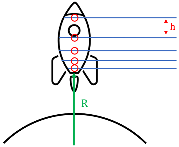
Imagine a space ship containing a collection of highly-accurate atomic clocks factory-set to arbitrary precision at the space-ship factory before launch. The clocks are lined up with precisely-equal spacing along the axis of the space ship, which should allow the astronauts to study events in spacetime to high accuracy as they orbit neutron stars or black holes. Despite all the precision, spacetime itself will conspire to detune the clocks. Yet all is not lost. Using the physics of nonlinear synchronization, the astronauts can bring all the clocks together to a compromise frequency—locking all the clocks to a common rate. This blog post shows how this can happen.
Fig.1 The high-precision space ship with a line of clocks.
Synchronization of Oscillators
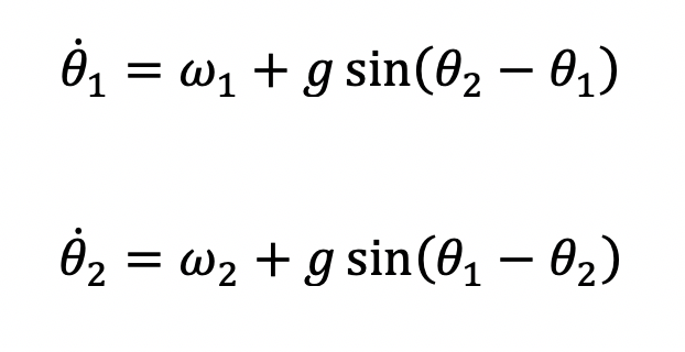
The simplest synchronization problem is two “phase oscillators” coupled with a symmetric nonlinearity. The dynamical flow is
where ωk are the individual angular frequencies and g is the coupling constant. When g is greater than the difference Δω, then the two oscillators, despite having different initial frequencies, will find a stable fixed point and lock to a compromise frequency.
Taking this model to N phase oscillators creates the well-known Kuramoto model that is characterized by a relatively sharp mean-field phase transition leading to global synchronization. The model averages N phase oscillators to a mean field where g is the coupling coefficient, K is the mean amplitude, Θ is the mean phase, and ω-bar is the mean frequency. The dynamics are given by
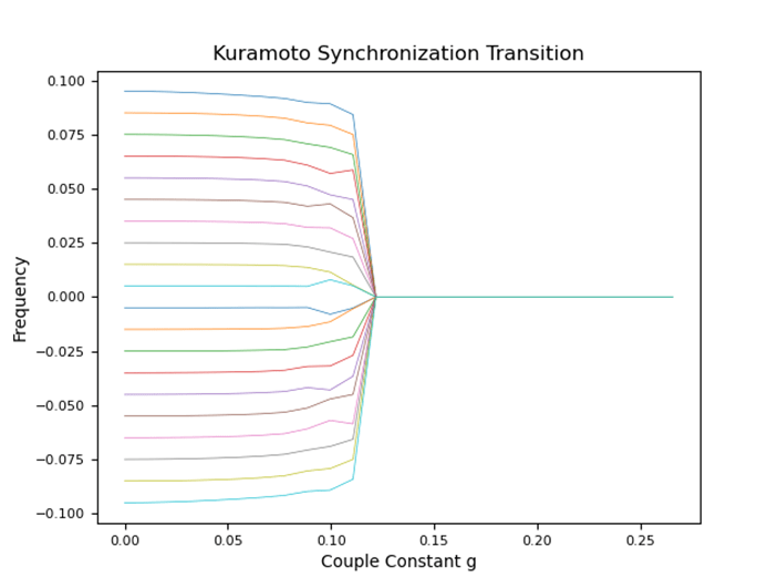
The last equation is the final mean-field equation that synchronizes each individual oscillator to the mean field. For a large number of oscillators that are globally coupled to each other, increasing the coupling has little effect on the oscillators until a critical threshold is crossed, after which all the oscillators synchronize with each other. This is known as the Kuramoto synchronization transition, shown in Fig. 2 for 20 oscillators with uniformly distributed initial frequencies. Note that the critical coupling constant gc is roughly half of the spread of initial frequencies.
Fig. 2 Entrainment graph of the Kuramoto transition for evenly distributed clock frequencies. N = 20.
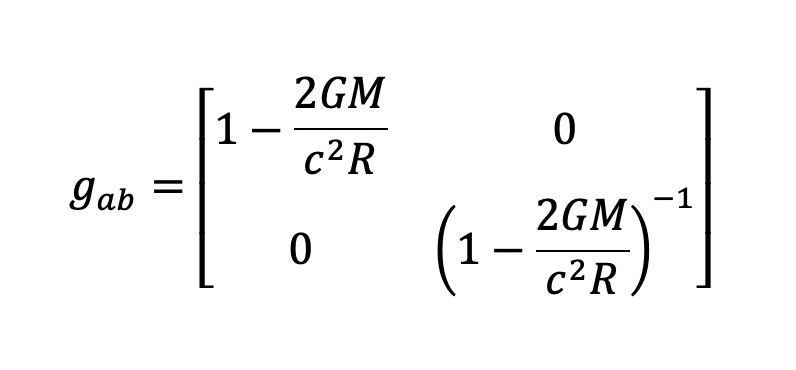
The question that this blog seeks to answer is how this synchronization mechanism may be used in a space craft exploring the strong gravity around neutron stars or black holes. The key to answering this question is the metric tensor for this system
where the first term is the time-like term g00 that affects ticking clocks, and the second term is the space-like term that affects the length of the space craft.
Kuramoto versus the Neutron Star
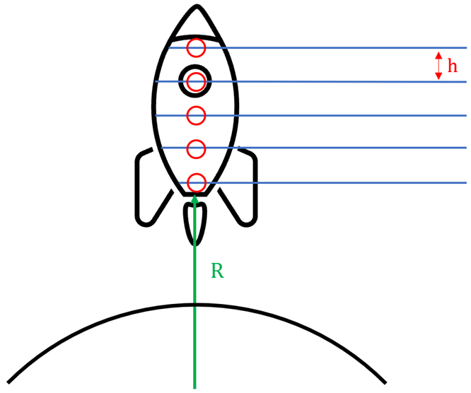
Consider the space craft holding a steady radius above a neutron star, as in Fig. 3. For simplicity, hold the craft stationary rather than in an orbit to remove the details of rotating frames. Because each clock is at a different gravitational potential, it runs at a different rate because of gravitational time dilation–clocks nearer to the neutron star run slower than clocks farther away. There is also a gravitational length contraction of the space craft, which modifies the clock rates as well.
Fig. 3 The space ship orbiting a neutron star. Each identical clock is at a different gravitational potential, causing them to run at different rates.
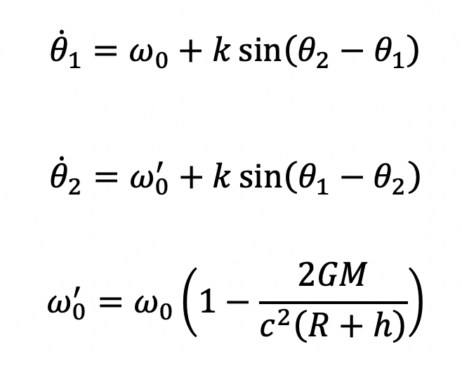
The analysis starts by incorporating the first-order approximation of time dilation through the component g00. The component is brought in through the period of oscillations. All frequencies are referenced to the base oscillator that has the angular rate ω0, and the other frequencies are primed. As we consider oscillators higher in the space craft at positions R + h, the 1/(R+h) term in g00 decreases as does the offset between each successive oscillator.
The dynamical equations for a system for only two clocks, coupled through the constant k, are
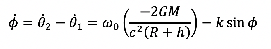
These are combined to a single equation by considering the phase difference
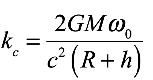
The two clocks will synchronize to a compromise frequency for the critical coupling coefficient
Now, if there is a string of N clocks, as in Fig. 3, the question is how the frequencies will spread out by gravitational time dilation, and what the entrainment of the frequencies to a common compromise frequency looks like. If the ship is located at some distance from the neutron star, then the gravitational potential at one clock to the next is approximately linear, and coupling them would produce the classic Kuramoto transition.
However, if the ship is much closer to the neutron star, so that the gravitational potential is no longer linear, then there is a “fan-out” of frequencies, with the bottom-most clock ticking much more slowly than the top-most clock. Coupling these clocks produces a modified, or “stretched”, Kuramoto transition as in Fig. 4.
Fig. 4 The “stretched” Kuramoto transition for N = 20 clocks near a neutron star. The bottom-most clock is just above the surface of the neutron star (left) and at twice that height (right). The spatial separation of the clocks in these examples is RS/20, and R0 is the radial position of the bottom-most clock.
In the two examples in Fig. 4, the bottom-most clock is just above the radius of the neutron star (at R0 = 4RS for a solar-mass neutron star, where RS is the Schwarzschild radius) and at twice that radius (at R0 = 8RS). The length of the ship, along which the clocks are distributed, is RS in this example. This may seem unrealistically large, but we could imagine a regular-sized ship supporting a long stiff cable dangling below it composed of carbon nanotubes that has the clocks distributed evenly on it, with the bottom-most clock at the radius R0. In fact, this might be a reasonable design for exploring spacetime events near a neutron star (although even carbon nanotubes would not be able to withstand the strain).
Kuramoto versus the Black Hole
Against expectation, exploring spacetime around a black hole is actually easier than around a neutron star, because there is no physical surface at the Schwarzschild radius RS, and gravitational tidal forces can be small for large black holes. In fact, one of the most unintuitive aspects of black holes pertains to a space ship falling into one. A distant observer sees the space ship contracting to zero length and the clocks slowing down and stopping as the space ship approaches the Schwarzschild radius asymptotically, but never crossing it. However, on board the ship, all appears normal as it crosses the Schwarzschild radius. To the astronaut inside, there is is a gravitational potential inside the space ship that causes the clocks at the base to run more slowly than the upper clocks, and length contraction affects the spacing a little, but otherwise there is no singularity as the event horizon is passed. This appears as a classic “paradox” of physics, with two different observers seeing paradoxically different behaviors.
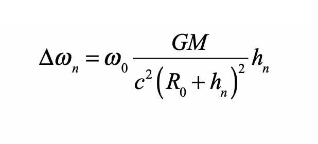
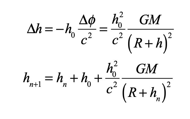
The resolution of this paradox lies in the differential geometry of the two observers. Each approximates spacetime with a Euclidean coordinate system that matches the local coordinates. The distant observer references the warped geometry to this “chart”, which produces the apparent divergence of the Schwarzschild metric at RS. However, the astronaut inside the space ship has her own flat chart to which she references the locally warped space time around the ship. Therefore, it is the differential changes, referenced to the ships coordinate origin, that capture gravitational time dilation and length contraction. Because the synchronization takes place in the local coordinate system of the ship, this is the coordinate system that goes into the dynamical equations for synchronization. Taking this approach, the shifts in the clock rates are given by the derivative of the metric as
where hn is the height of the n-th clock above R0.
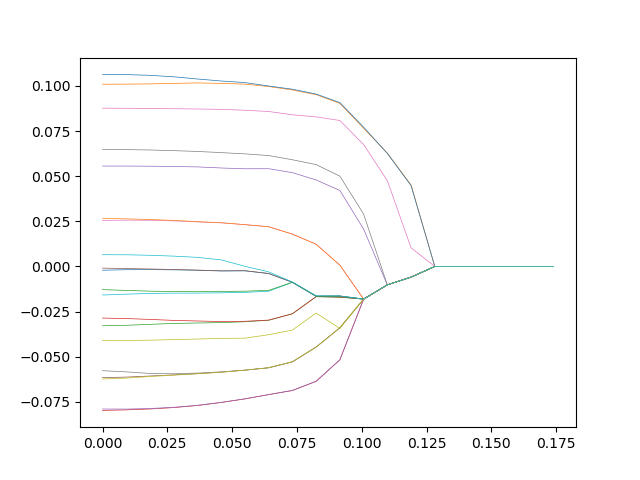
Fig. 5 shows the entrainment plot for the black hole. The plot noticeably has a much smoother transition. In this higher mass case, the system does not have as many hard coupling transitions and instead exhibits smooth behavior for global coupling. This is the Kuramoto “cascade”. Contrast the behavior of Fig. 5 (left) to the classic Kuramoto transition of Fig. 2. The increasing frequency separations near the black hole produces a succession of frequency locks as the coupling coefficient increases. For comparison, the case of linear coupling along the cable is shown in Fig. 5 on the right. The cascade is now accompanied with interesting oscillations as one clock entrains with a neighbor, only to be pulled back by interaction with locked subclusters.
Fig. 5 The Kuramoto cascade for R0 = 1RS for global coupling (left) and linear coupling (right).
Now let us consider what role the spatial component of the metric tensor plays in the synchronization. The spatial component causes the space between the oscillators to decrease closer to the supermassive object. This would cause the oscillators to entrain faster because the bottom oscillators that entrain the slowest would be closer together, but the top oscillators would entrain slower since they are a farther distance apart, as in Fig. 6.
Fig. 6 The space ship experiencing gravitational length contraction that changes the separations among the clocks and further changes their respective gravitational potentials and clock rates.
In terms of the local coordinates of the space ship, the locations of each clock are
These values for hn can be put into the equation for ωn above. But it is clear that this produces a second order effect. Even at the event horizon, this effect is only a fraction of the shifts caused by g00 directly on the clocks. This is in contrast to what a distant observer sees–the clock separations decreasing to zero, which would seem to decrease the frequency shifts. But the synchronization coupling is performed in the ship frame, not the distant frame, so the astronaut can safely ignore this contribution.
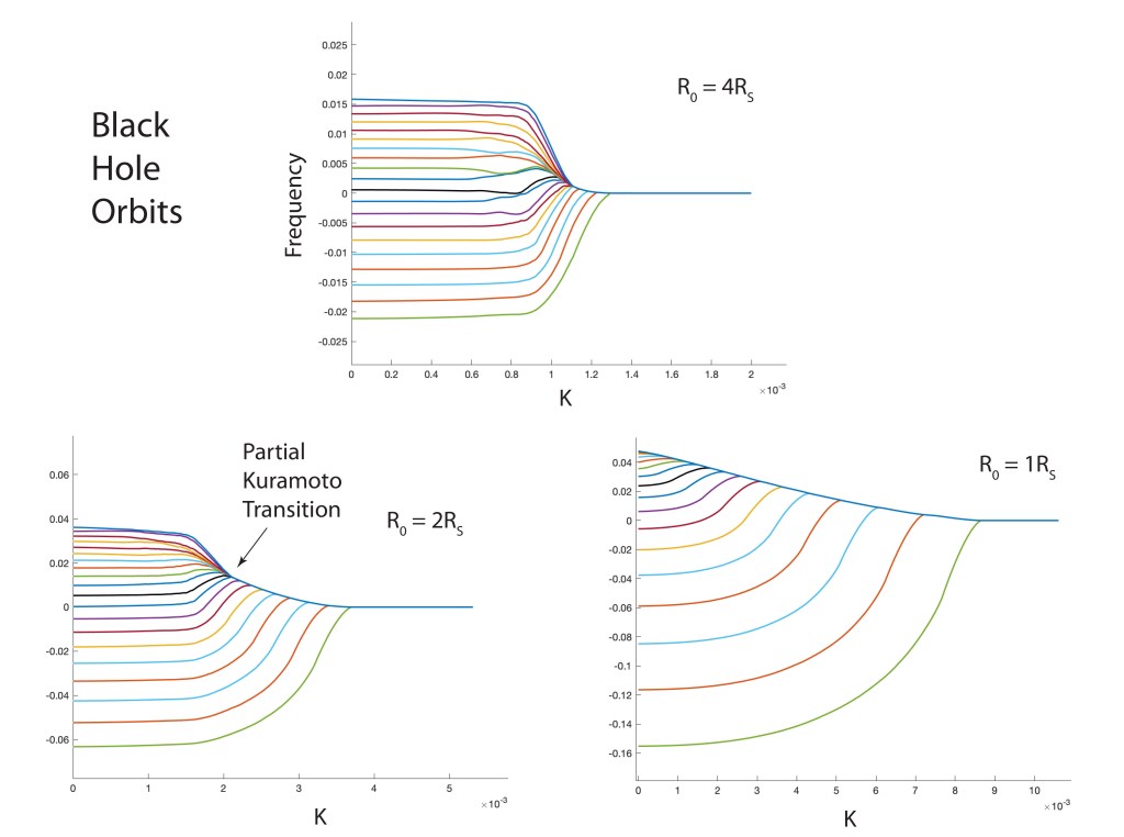
As a final exploration of the black hole, before we leave it behind, look at the behavior for different values of R0 in Fig. 7. At 4RS, the Kuramoto transition is stretched. At 2RS there is a partial Kuramoto transition for the upper clocks, that then stretch into a cascade of locking events for the lower clocks. At 1RS we see the full cascade as before.
Fig. 7 The Kuramoto transition stretches into a cascade as the radius approaches the event horizon.
Note from the Editor:
This blog post by Moira Andrews is based on her final project for Phys 411, upper division undergraduate mechanics, at Purdue University. Students are asked to combine two seemingly-unrelated aspects of modern dynamics and explore the results. Moira thought of synchronizing clocks that are experiencing gravitational time dilation near a massive body. This is a nice example of how GR combined with nonlinear synchronization yields the novel phenomenon of a “synchronization cascade”.
Bibliography
Cheng, T.-P. (2010). Relativity, Gravitation and Cosmology. Oxford University Press.
Keeton, C. (2014). Principles of Astrophysics. Springer.
Marmet, P. (n.d.). Natural Length Contraction Due to Gravity. Newton Physics – Links to Papers, Books and Web Sites. Retrieved April 27, 2021, from https://newtonphysics.on.ca/gravity/index.html
Nolte, D. D. (2019). Introduction to Modern Dynamics (2nd ed.). Oxford University Press, USA.
This Blog Post is a Companion to the undergraduate physics textbook Modern Dynamics: Chaos, Networks, Space and Time, 2nd ed. (Oxford, 2019) introducing Lagrangians and Hamiltonians, chaos theory, complex systems, synchronization, neural networks, econophysics and Special and General Relativity.
It is surprising how much of modern dynamics boils down to an extremely simple formula
This innocuous-looking equation carries such riddles, such surprises, such unintuitive behavior that it can become the object of study for life. This equation is called a vector flow equation, and it can be used to capture the essential physics of economies, neurons, ecosystems, networks, and even orbits of photons around black holes. This equation is to modern dynamics what F = ma was to classical mechanics. It is the starting point for understanding complex systems.
The Magic of Phase Space
The apparent simplicity of the “flow equation” masks the complexity it contains. It is a vector equation because each “dimension” is a variable of a complex system. Many systems of interest may have only a few variables, but ecosystems and economies and social networks may have hundreds or thousands of variables. Expressed in component format, the flow equation is
where the superscript spans the number of variables. But even this masks all that can happen with such an equation. Each of the functions fa can be entirely different from each other, and can be any type of function, whether polynomial, rational, algebraic, transcendental or composite, although they must be single-valued. They are generally nonlinear, and the limitless ways that functions can be nonlinear is where the richness of the flow equation comes from.
The vector flow equation is an ordinary differential equation (ODE) that can be solved for specific trajectories as initial value problems. A single set of initial conditions defines a unique trajectory. For instance, the trajectory for a 4-dimensional example is described as the column vector
which is the single-parameter position vector to a point in phase space, also called state space. The point sweeps through successive configurations as a function of its single parameter—time. This trajectory is also called an orbit. In classical mechanics, the focus has tended to be on the behavior of specific orbits that arise from a specific set of initial conditions. This is the classic “rock thrown from a cliff” problem of introductory physics courses. However, in modern dynamics, the focus shifts away from individual trajectories to encompass the set of all possible trajectories.
Why is Modern Dynamics part of Physics?
If finding the solutions to the “x-dot equals f” vector flow equation is all there is to do, then this would just be a math problem—the solution of ODE’s. There are plenty of gems for mathematicians to look for, and there is an entire of field of study in mathematics called “dynamical systems“, but this would not be “physics”. Physics as a profession is separate and distinct from mathematics, although the two are sometimes confused. Physics uses mathematics as its language and as its toolbox, but physics is not mathematics. Physics is done best when it is done qualitatively—this means with scribbles done on napkins in restaurants or on the back of envelopes while waiting in line. Physics is about recognizing relationships and patterns. Physics is about identifying the limits to scaling properties where the physics changes when scales change. Physics is about the mapping of the simplest possible mathematics onto behavior in the physical world, and recognizing when the simplest possible mathematics is a universal that applies broadly to diverse systems that seem different, but that share the same underlying principles.
So, granted solving ODE’s is not physics, there is still a tremendous amount of good physics that can be done by solving ODE’s. ODE solvers become the modern physicist’s experimental workbench, providing data output from numerical experiments that can test the dependence on parameters in ways that real-world experiments might not be able to access. Physical intuition can be built based on such simulations as the engaged physicist begins to “understand” how the system behaves, able to explain what will happen as the values of parameters are changed.
In the follow sections, three examples of modern dynamics are introduced with a preliminary study, including Python code. These examples are: Galactic dynamics, synchronized networks and ecosystems. Despite their very different natures, their description using dynamical flows share features in common and illustrate the beauty and depth of behavior that can be explored with simple equations.
Galactic Dynamics
One example of the power and beauty of the vector flow equation and its set of all solutions in phase space is called the Henon-Heiles model of the motion of a star within a galaxy. Of course, this is a terribly complicated problem that involves tens of billions of stars, but if you average over the gravitational potential of all the other stars, and throw in a couple of conservation laws, the resulting potential can look surprisingly simple. The motion in the plane of this galactic potential takes two configuration coordinates (x, y) with two associated momenta (px, py) for a total of four dimensions. The flow equations in four-dimensional phase space are simply
Fig. 1 The 4-dimensional phase space flow equations of a star in a galaxy. The terms in light blue are a simple two-dimensional harmonic oscillator. The terms in magenta are the nonlinear contributions from the stars in the galaxy.
where the terms in the light blue box describe a two-dimensional simple harmonic oscillator (SHO), which is a linear oscillator, modified by the terms in the magenta box that represent the nonlinear galactic potential. The orbits of this Hamiltonian system are chaotic, and because there is no dissipation in the model, a single orbit will continue forever within certain ranges of phase space governed by energy conservation, but never quite repeating.
Fig. 2 Two-dimensional Poincaré section of sets of trajectories in four-dimensional phase space for the Henon-Heiles galactic dynamics model. The perturbation parameter is &eps; = 0.3411 and the energy E = 1.
#!/usr/bin/env python3
# -*- coding: utf-8 -*-
"""
Hamilton4D.py
Created on Wed Apr 18 06:03:32 2018

@author: nolte

Derived from:
D. D. Nolte, Introduction to Modern Dynamics: Chaos, Networks, Space and Time, 2nd ed. (Oxford,2019)
"""

import numpy as np
import matplotlib as mpl
from mpl_toolkits.mplot3d import Axes3D
from scipy import integrate
from matplotlib import pyplot as plt
from matplotlib import cm
import time
import os

plt.close('all')

# model_case 1 = Heiles
# model_case 2 = Crescent
print(' ')
print('Hamilton4D.py')
print('Case: 1 = Heiles')
print('Case: 2 = Crescent')
model_case = int(input('Enter the Model Case (1-2)'))

if model_case == 1:
    E = 1       # Heiles: 1, 0.3411   Crescent: 0.05, 1
    epsE = 0.3411   # 3411
    def flow_deriv(x_y_z_w,tspan):
        x, y, z, w = x_y_z_w
        a = z
        b = w
        c = -x - epsE*(2*x*y)
        d = -y - epsE*(x**2 - y**2)
        return[a,b,c,d]
else:
    E = .1       #   Crescent: 0.1, 1
    epsE = 1
    def flow_deriv(x_y_z_w,tspan):
        x, y, z, w = x_y_z_w
        a = z
        b = w
        c = -(epsE*(y-2*x**2)*(-4*x) + x)
        d = -(y-epsE*2*x**2)
        return[a,b,c,d]

prms = np.sqrt(E)
pmax = np.sqrt(2*E)

# Potential Function
if model_case == 1:
    V = np.zeros(shape=(100,100))
    for xloop in range(100):
        x = -2 + 4*xloop/100
        for yloop in range(100):
            y = -2 + 4*yloop/100
            V[yloop,xloop] = 0.5*x**2 + 0.5*y**2 + epsE*(x**2*y - 0.33333*y**3)
else:
    V = np.zeros(shape=(100,100))
    for xloop in range(100):
        x = -2 + 4*xloop/100
        for yloop in range(100):
            y = -2 + 4*yloop/100
            V[yloop,xloop] = 0.5*x**2 + 0.5*y**2 + epsE*(2*x**4 - 2*x**2*y)

fig = plt.figure(1)
contr = plt.contourf(V,100, cmap=cm.coolwarm, vmin = 0, vmax = 10)
fig.colorbar(contr, shrink=0.5, aspect=5)
fig = plt.show()

repnum = 250
mulnum = 64/repnum

np.random.seed(1)
for reploop  in range(repnum):
    px1 = 2*(np.random.random((1))-0.499)*pmax
    py1 = np.sign(np.random.random((1))-0.499)*np.real(np.sqrt(2*(E-px1**2/2)))
    xp1 = 0
    yp1 = 0

    x_y_z_w0 = [xp1, yp1, px1, py1]

    tspan = np.linspace(1,1000,10000)
    x_t = integrate.odeint(flow_deriv, x_y_z_w0, tspan)
    siztmp = np.shape(x_t)
    siz = siztmp[0]

    if reploop % 50 == 0:
        plt.figure(2)
        lines = plt.plot(x_t[:,0],x_t[:,1])
        plt.setp(lines, linewidth=0.5)
        plt.show()
        time.sleep(0.1)
        #os.system("pause")

    y1 = x_t[:,0]
    y2 = x_t[:,1]
    y3 = x_t[:,2]
    y4 = x_t[:,3]

    py = np.zeros(shape=(2*repnum,))
    yvar = np.zeros(shape=(2*repnum,))
    cnt = -1
    last = y1[1]
    for loop in range(2,siz):
        if (last < 0)and(y1[loop] > 0):
            cnt = cnt+1
            del1 = -y1[loop-1]/(y1[loop] - y1[loop-1])
            py[cnt] = y4[loop-1] + del1*(y4[loop]-y4[loop-1])
            yvar[cnt] = y2[loop-1] + del1*(y2[loop]-y2[loop-1])
            last = y1[loop]
        else:
            last = y1[loop]

    plt.figure(3)
    lines = plt.plot(yvar,py,'o',ms=1)
    plt.show()

if model_case == 1:
    plt.savefig('Heiles')
else:
    plt.savefig('Crescent')
Networks, Synchronization and Emergence
A central paradigm of nonlinear science is the emergence of patterns and organized behavior from seemingly random interactions among underlying constituents. Emergent phenomena are among the most awe inspiring topics in science. Crystals are emergent, forming slowly from solutions of reagents. Life is emergent, arising out of the chaotic soup of organic molecules on Earth (or on some distant planet). Intelligence is emergent, and so is consciousness, arising from the interactions among billions of neurons. Ecosystems are emergent, based on competition and symbiosis among species. Economies are emergent, based on the transfer of goods and money spanning scales from the local bodega to the global economy.
One of the common underlying properties of emergence is the existence of networks of interactions. Networks and network science are topics of great current interest driven by the rise of the World Wide Web and social networks. But networks are ubiquitous and have long been the topic of research into complex and nonlinear systems. Networks provide a scaffold for understanding many of the emergent systems. It allows one to think of isolated elements, like molecules or neurons, that interact with many others, like the neighbors in a crystal or distant synaptic connections.
From the point of view of modern dynamics, the state of a node can be a variable or a “dimension” and the interactions among links define the functions of the vector flow equation. Emergence is then something that “emerges” from the dynamical flow as many elements interact through complex networks to produce simple or emergent patterns.
Synchronization is a form of emergence that happens when lots of independent oscillators, each vibrating at their own personal frequency, are coupled together to push and pull on each other, entraining all the individual frequencies into one common global oscillation of the entire system. Synchronization plays an important role in the solar system, explaining why the Moon always shows one face to the Earth, why Saturn’s rings have gaps, and why asteroids are mainly kept away from colliding with the Earth. Synchronization plays an even more important function in biology where it coordinates the beating of the heart and the functioning of the brain.
One of the most dramatic examples of synchronization is the Kuramoto synchronization phase transition. This occurs when a large set of individual oscillators with differing natural frequencies interact with each other through a weak nonlinear coupling. For small coupling, all the individual nodes oscillate at their own frequency. But as the coupling increases, there is a sudden coalescence of all the frequencies into a single common frequency. This mechanical phase transition, called the Kuramoto transition, has many of the properties of a thermodynamic phase transition, including a solution that utilizes mean field theory.
Fig. 3 The Kuramoto model for the nonlinear coupling of N simple phase oscillators. The term in light blue is the simple phase oscillator. The term in magenta is the global nonlinear coupling that connects each oscillator to every other.
The simulation of 20 Poncaré phase oscillators with global coupling is shown in Fig. 4 as a function of increasing coupling coefficient g. The original individual frequencies are spread randomly. The oscillators with similar frequencies are the first to synchronize, forming small clumps that then synchronize with other clumps of oscillators, until all oscillators are entrained to a single compromise frequency. The Kuramoto phase transition is not sharp in this case because the value of N = 20 is too small. If the simulation is run for 200 oscillators, there is a sudden transition from unsynchronized to synchronized oscillation at a threshold value of g.
Fig. 4 The Kuramoto model for 20 Poincare oscillators showing the frequencies as a function of the coupling coefficient.
The Kuramoto phase transition is one of the most important fundamental examples of modern dynamics because it illustrates many facets of nonlinear dynamics in a very simple way. It highlights the importance of nonlinearity, the simplification of phase oscillators, the use of mean field theory, the underlying structure of the network, and the example of a mechanical analog to a thermodynamic phase transition. It also has analytical solutions because of its simplicity, while still capturing the intrinsic complexity of nonlinear systems.
#!/usr/bin/env python3
# -*- coding: utf-8 -*-
"""
Created on Sat May 11 08:56:41 2019

@author: nolte

D. D. Nolte, Introduction to Modern Dynamics: Chaos, Networks, Space and Time, 2nd ed. (Oxford,2019)
"""

# https://www.python-course.eu/networkx.php
# https://networkx.github.io/documentation/stable/tutorial.html
# https://networkx.github.io/documentation/stable/reference/functions.html

import numpy as np
from scipy import integrate
from matplotlib import pyplot as plt
import networkx as nx
from UserFunction import linfit
import time

tstart = time.time()

plt.close('all')

Nfac = 25   # 25
N = 50      # 50
width = 0.2

# model_case 1 = complete graph (Kuramoto transition)
# model_case 2 = Erdos-Renyi
model_case = int(input('Input Model Case (1-2)'))
if model_case == 1:
    facoef = 0.2
    nodecouple = nx.complete_graph(N)
elif model_case == 2:
    facoef = 5
    nodecouple = nx.erdos_renyi_graph(N,0.1)


# function: omegout, yout = coupleN(G)
def coupleN(G):

    # function: yd = flow_deriv(x_y)
    def flow_deriv(y,t0):

        yp = np.zeros(shape=(N,))
        for omloop  in range(N):
            temp = omega[omloop]
            linksz = G.node[omloop]['numlink']
            for cloop in range(linksz):
                cindex = G.node[omloop]['link'][cloop]
                g = G.node[omloop]['coupling'][cloop]

                temp = temp + g*np.sin(y[cindex]-y[omloop])

            yp[omloop] = temp

        yd = np.zeros(shape=(N,))
        for omloop in range(N):
            yd[omloop] = yp[omloop]

        return yd
    # end of function flow_deriv(x_y)

    mnomega = 1.0

    for nodeloop in range(N):
        omega[nodeloop] = G.node[nodeloop]['element']

    x_y_z = omega

    # Settle-down Solve for the trajectories
    tsettle = 100
    t = np.linspace(0, tsettle, tsettle)
    x_t = integrate.odeint(flow_deriv, x_y_z, t)
    x0 = x_t[tsettle-1,0:N]

    t = np.linspace(1,1000,1000)
    y = integrate.odeint(flow_deriv, x0, t)
    siztmp = np.shape(y)
    sy = siztmp[0]

    # Fit the frequency
    m = np.zeros(shape = (N,))
    w = np.zeros(shape = (N,))
    mtmp = np.zeros(shape=(4,))
    btmp = np.zeros(shape=(4,))
    for omloop in range(N):

        if np.remainder(sy,4) == 0:
            mtmp[0],btmp[0] = linfit(t[0:sy//2],y[0:sy//2,omloop]);
            mtmp[1],btmp[1] = linfit(t[sy//2+1:sy],y[sy//2+1:sy,omloop]);
            mtmp[2],btmp[2] = linfit(t[sy//4+1:3*sy//4],y[sy//4+1:3*sy//4,omloop]);
            mtmp[3],btmp[3] = linfit(t,y[:,omloop]);
        else:
            sytmp = 4*np.floor(sy/4);
            mtmp[0],btmp[0] = linfit(t[0:sytmp//2],y[0:sytmp//2,omloop]);
            mtmp[1],btmp[1] = linfit(t[sytmp//2+1:sytmp],y[sytmp//2+1:sytmp,omloop]);
            mtmp[2],btmp[2] = linfit(t[sytmp//4+1:3*sytmp/4],y[sytmp//4+1:3*sytmp//4,omloop]);
            mtmp[3],btmp[3] = linfit(t[0:sytmp],y[0:sytmp,omloop]);


        #m[omloop] = np.median(mtmp)
        m[omloop] = np.mean(mtmp)

        w[omloop] = mnomega + m[omloop]

    omegout = m
    yout = y

    return omegout, yout
    # end of function: omegout, yout = coupleN(G)


Nlink = N*(N-1)//2
omega = np.zeros(shape=(N,))
omegatemp = width*(np.random.rand(N)-1)
meanomega = np.mean(omegatemp)
omega = omegatemp - meanomega
sto = np.std(omega)

lnk = np.zeros(shape = (N,), dtype=int)
for loop in range(N):
    nodecouple.node[loop]['element'] = omega[loop]
    nodecouple.node[loop]['link'] = list(nx.neighbors(nodecouple,loop))
    nodecouple.node[loop]['numlink'] = np.size(list(nx.neighbors(nodecouple,loop)))
    lnk[loop] = np.size(list(nx.neighbors(nodecouple,loop)))

avgdegree = np.mean(lnk)
mnomega = 1

facval = np.zeros(shape = (Nfac,))
yy = np.zeros(shape=(Nfac,N))
xx = np.zeros(shape=(Nfac,))
for facloop in range(Nfac):
    print(facloop)

    fac = facoef*(16*facloop/(Nfac))*(1/(N-1))*sto/mnomega
    for nodeloop in range(N):
        nodecouple.node[nodeloop]['coupling'] = np.zeros(shape=(lnk[nodeloop],))
        for linkloop in range (lnk[nodeloop]):
            nodecouple.node[nodeloop]['coupling'][linkloop] = fac

    facval[facloop] = fac*avgdegree

    omegout, yout = coupleN(nodecouple)                           # Here is the subfunction call for the flow

    for omloop in range(N):
        yy[facloop,omloop] = omegout[omloop]

    xx[facloop] = facval[facloop]

plt.figure(1)
lines = plt.plot(xx,yy)
plt.setp(lines, linewidth=0.5)
plt.show()

elapsed_time = time.time() - tstart
print('elapsed time = ',format(elapsed_time,'.2f'),'secs')
The Web of Life
Ecosystems are among the most complex systems on Earth. The complex interactions among hundreds or thousands of species may lead to steady homeostasis in some cases, to growth and collapse in other cases, and to oscillations or chaos in yet others. But the definition of species can be broad and abstract, referring to businesses and markets in economic ecosystems, or to cliches and acquaintances in social ecosystems, among many other examples. These systems are governed by the laws of evolutionary dynamics that include fitness and survival as well as adaptation.
The dimensionality of the dynamical spaces for these systems extends to hundreds or thousands of dimensions—far too complex to visualize when thinking in four dimensions is already challenging. Yet there are shared principles and common behaviors that emerge even here. Many of these can be illustrated in a simple three-dimensional system that is represented by a triangular simplex that can be easily visualized, and then generalized back to ultra-high dimensions once they are understood.
A simplex is a closed (N-1)-dimensional geometric figure that describes a zero-sum game (game theory is an integral part of evolutionary dynamics) among N competing species. For instance, a two-simplex is a triangle that captures the dynamics among three species. Each vertex of the triangle represents the situation when the entire ecosystem is composed of a single species. Anywhere inside the triangle represents the situation when all three species are present and interacting.
A classic model of interacting species is the replicator equation. It allows for a fitness-based proliferation and for trade-offs among the individual species. The replicator dynamics equations are shown in Fig. 5.
Fig. 5 Replicator dynamics has a surprisingly simple form, but with surprisingly complicated behavior. The key elements are the fitness and the payoff matrix. The fitness relates to how likely the species will survive. The payoff matrix describes how one species gains at the loss of another (although symbiotic relationships also occur).
The population dynamics on the 2D simplex are shown in Fig. 6 for several different pay-off matrices. The matrix values are shown in color and help interpret the trajectories. For instance the simplex on the upper-right shows a fixed point center. This reflects the antisymmetric character of the pay-off matrix around the diagonal. The stable spiral on the lower-left has a nearly asymmetric pay-off matrix, but with unequal off-diagonal magnitudes. The other two cases show central saddle points with stable fixed points on the boundary. A very large variety of behaviors are possible for this very simple system. The Python program is shown in Trirep.py.
Fig. 6 Payoff matrix and population simplex for four random cases: Upper left is an unstable saddle. Upper right is a center. Lower left is a stable spiral. Lower right is a marginal case.
#!/usr/bin/env python3
# -*- coding: utf-8 -*-
"""
trirep.py
Created on Thu May  9 16:23:30 2019

@author: nolte

Derived from:
D. D. Nolte, Introduction to Modern Dynamics: Chaos, Networks, Space and Time, 2nd ed. (Oxford,2019)
"""

import numpy as np
from scipy import integrate
from matplotlib import pyplot as plt

plt.close('all')

def tripartite(x,y,z):

    sm = x + y + z
    xp = x/sm
    yp = y/sm

    f = np.sqrt(3)/2

    y0 = f*xp
    x0 = -0.5*xp - yp + 1;

    plt.figure(2)
    lines = plt.plot(x0,y0)
    plt.setp(lines, linewidth=0.5)
    plt.plot([0, 1],[0, 0],'k',linewidth=1)
    plt.plot([0, 0.5],[0, f],'k',linewidth=1)
    plt.plot([1, 0.5],[0, f],'k',linewidth=1)
    plt.show()


def solve_flow(y,tspan):
    def flow_deriv(y, t0):
    #"""Compute the time-derivative ."""

        f = np.zeros(shape=(N,))
        for iloop in range(N):
            ftemp = 0
            for jloop in range(N):
                ftemp = ftemp + A[iloop,jloop]*y[jloop]
            f[iloop] = ftemp

        phitemp = phi0          # Can adjust this from 0 to 1 to stabilize (but Nth population is no longer independent)
        for loop in range(N):
            phitemp = phitemp + f[loop]*y[loop]
        phi = phitemp

        yd = np.zeros(shape=(N,))
        for loop in range(N-1):
            yd[loop] = y[loop]*(f[loop] - phi);

        if np.abs(phi0) < 0.01:             # average fitness maintained at zero
            yd[N-1] = y[N-1]*(f[N-1]-phi);
        else:                                     # non-zero average fitness
            ydtemp = 0
            for loop in range(N-1):
                ydtemp = ydtemp - yd[loop]
            yd[N-1] = ydtemp

        return yd

    # Solve for the trajectories
    t = np.linspace(0, tspan, 701)
    x_t = integrate.odeint(flow_deriv,y,t)
    return t, x_t

# model_case 1 = zero diagonal
# model_case 2 = zero trace
# model_case 3 = asymmetric (zero trace)
print(' ')
print('trirep.py')
print('Case: 1 = antisymm zero diagonal')
print('Case: 2 = antisymm zero trace')
print('Case: 3 = random')
model_case = int(input('Enter the Model Case (1-3)'))

N = 3
asymm = 3      # 1 = zero diag (replicator eqn)   2 = zero trace (autocatylitic model)  3 = random (but zero trace)
phi0 = 0.001            # average fitness (positive number) damps oscillations
T = 100;


if model_case == 1:
    Atemp = np.zeros(shape=(N,N))
    for yloop in range(N):
        for xloop in range(yloop+1,N):
            Atemp[yloop,xloop] = 2*(0.5 - np.random.random(1))
            Atemp[xloop,yloop] = -Atemp[yloop,xloop]

if model_case == 2:
    Atemp = np.zeros(shape=(N,N))
    for yloop in range(N):
        for xloop in range(yloop+1,N):
            Atemp[yloop,xloop] = 2*(0.5 - np.random.random(1))
            Atemp[xloop,yloop] = -Atemp[yloop,xloop]
        Atemp[yloop,yloop] = 2*(0.5 - np.random.random(1))
    tr = np.trace(Atemp)
    A = Atemp
    for yloop in range(N):
        A[yloop,yloop] = Atemp[yloop,yloop] - tr/N

else:
    Atemp = np.zeros(shape=(N,N))
    for yloop in range(N):
        for xloop in range(N):
            Atemp[yloop,xloop] = 2*(0.5 - np.random.random(1))

    tr = np.trace(Atemp)
    A = Atemp
    for yloop in range(N):
        A[yloop,yloop] = Atemp[yloop,yloop] - tr/N

plt.figure(3)
im = plt.matshow(A,3,cmap=plt.cm.get_cmap('seismic'))  # hsv, seismic, bwr
cbar = im.figure.colorbar(im)

M = 20
delt = 1/M
ep = 0.01;

tempx = np.zeros(shape = (3,))
for xloop in range(M):
    tempx[0] = delt*(xloop)+ep;
    for yloop in range(M-xloop):
        tempx[1] = delt*yloop+ep
        tempx[2] = 1 - tempx[0] - tempx[1]

        x0 = tempx/np.sum(tempx);          # initial populations

        tspan = 70
        t, x_t = solve_flow(x0,tspan)

        y1 = x_t[:,0]
        y2 = x_t[:,1]
        y3 = x_t[:,2]

        plt.figure(1)
        lines = plt.plot(t,y1,t,y2,t,y3)
        plt.setp(lines, linewidth=0.5)
        plt.show()
        plt.ylabel('X Position')
        plt.xlabel('Time')

        tripartite(y1,y2,y3)
Topics in Modern Dynamics
These three examples are just the tip of the iceberg. The topics in modern dynamics are almost numberless. Any system that changes in time is a potential object of study in modern dynamics. Here is a list of a few topics that spring to mind.