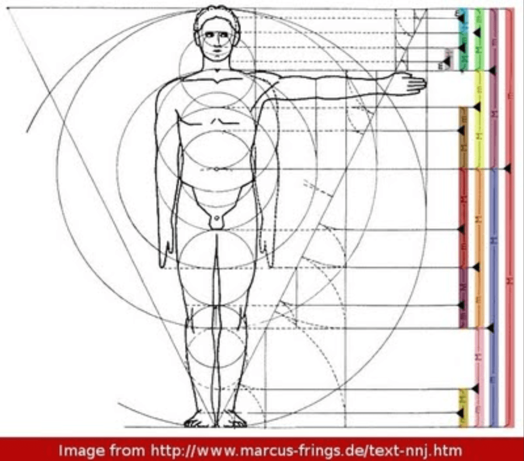
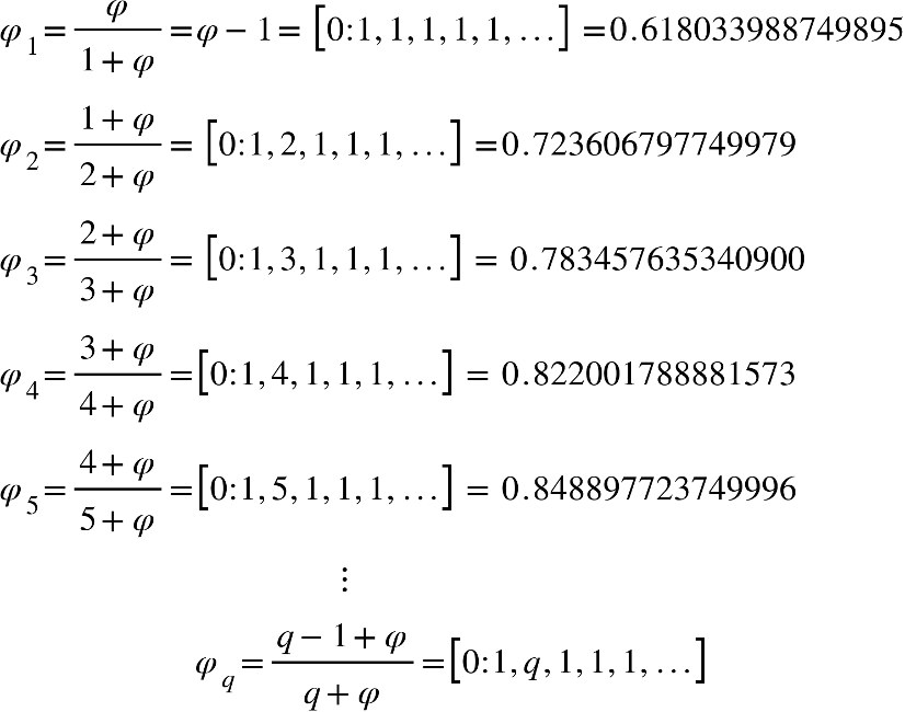
If ever there was a magic number that encoded the mysteries of the universe, then surely it must be the golden mean. It seems to pop up everywhere. In flowers and hurricanes. In pine cones and sea shells. In architecture and infinite sums. In telescoping cascades of golden rectangles in the human figure.
Fig. 1. The golden mean can be found in numerous ratios of the measurements of the human body.
It also rears its head in the world of chaos theory, governing how a twisting dumbbell rotor transitions from regular motion to chaotic motion when it is tapped gently at a regular period.
The Golden Ratio
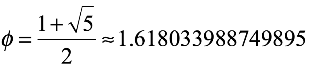
The Golden ratio can be defined in many ways, but its most common expression is given by
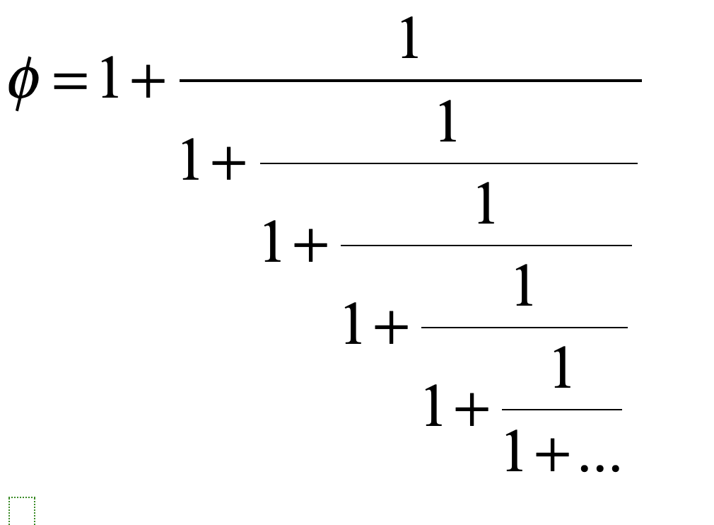
Among its many marvelous properties, one is that it is the hardest number to approximate with a ratio of small integers. For instance, the ratio 89/55 is a number that is as close as one part in ten thousand to the golden mean but it is hardly a ratio of small integers. This result may seem obscure, but there is a systematic way to find the ratios of integers that approximate an irrational number. This is known as continued fractions.
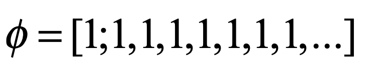
The continued fraction for the golden mean has an especially simple repeating form
also written as
This continued fraction has the slowest convergence for its continued fraction of any other number. Hence, the Golden Ratio can be considered, using this criterion, to be the most irrational number of all, and it governs the last straw of order as chaos emerges from a surprisingly simple map.
The Kicked Rigid Rotor
The rigid rotator (the simple dumbbell) is one of the iconic systems in physics. It is a classic object in the study of rotational dynamics, showing up in Lagrangian formulations as well as Euler’s equations. It is also a classic system in elementary quantum mechanics, illustrating the quantization of angular momentum. In the current setting (Hamiltonian chaos), it is an example of a periodically perturbed system that displays beautiful phenomena.
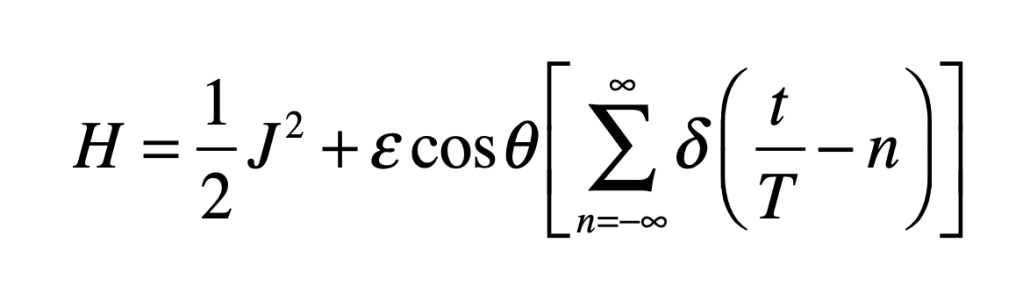
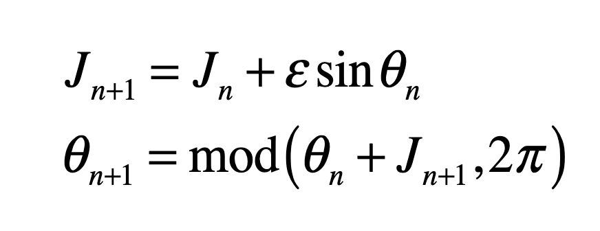
In chaos theory, the relationship between a continuous dynamical system and its discrete map is sometimes difficult to identify. However, a discrete map arises naturally from a randomly kicked dumbbell rotator. The system has an angular momentum J and a physical angle θ. The strength of the angular momentum kick is given by the perturbation parameter ε, and the torque of the kick is a function of the physical angle θ. The kicked rotator has the Hamiltonian
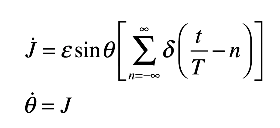
where the kicks are evenly timed with period T. The perturbation parameter ε can be large. The perturbation amplitude and sign depend on the instantaneous angle θ. The equations of motion from Hamilton’s equations are
The values for J and θ just before the nth successive kick are Jn and qn, respectively. Because the evaluation of the variables occurs at the period T, these discrete observations represent the values of a Poincaré section.
The Chirikov Twist Map
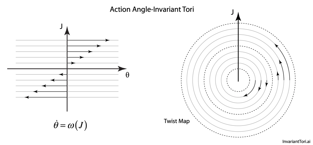
The phase space (in action-angle coordinates) of the rigid rotator is particularly attractive for applications because it is simply a linear flow that has increasing velocities with increasing action J. In action-angle representation, it is a twist map, where circles outside the radius for J = 0 twist in one direction but inside that radius they twist in the opposite direction. David Birkhoff showed in 1913, while proving Poincaré’s last geometric theorem, that a simple periodic perturbation of this system creates a set of closed trajectories (around an elliptical point) and a set of open trajectories (around a hyperbolic point).
Fig. 2. The action-angle phase space of a rigid rotator, plus the associated twist map.
The rotator dynamics are continuous between each kick, leading to the discrete map (known as the Standard Map or the Chirikov Map)
in which the rotator is “strobed”, or observed, at regular periods of 2π. When ε = 0, the orbits on the (θ, J) plane are simply horizontal lines—the rotator spins with regular motion at a speed determined by J.
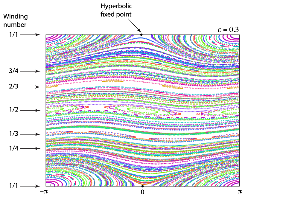
As the strength of the kick ε increases from zero, the Poicaré-Birkhoff theorem kicks in, and a first “island chain” appears with a single elliptical point paired with a single hyperbolic point. Then at larger values of ε new island chains appear, first with two islands, then with three, as in the figure below with ε = 0.3. Orbits that produce two islands are in a 2:1 resonance, and with three islands are in either a 3:1 or a 3:2 resonance. With increasing ε, more and more island chains open up, representing higher resonances.
Fig. 3 Chirikov map for ε = 0.3. The 1/1, 1/2 and 1/3 (2/3) island chains have opened with a primary hyperbolic point on the 1/1 resonance.
Each resonance is associated with a ratio of small integers: 1/2; 2/3; 3/4; 4/5 and beyond. These are the natural harmonics of the system. As the integers get larger, the ratios begin to approximate irrational numbers.
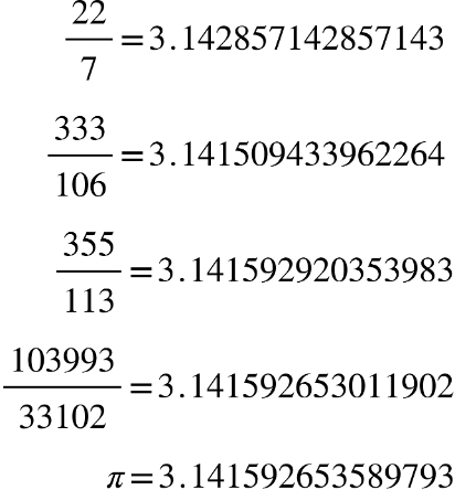
For instance, the number pi is approximated to increasing accuracy by the sequence of ratios:
Fig. Successive convergents of the irrational number pi.
These are called convergents and are obtained by taking more terms in the continued fraction representation of pi.
One of the fundamental findings of the theory of resonances in Hamiltonian systems is the decreasing “weight” of resonances associated with ratios of larger integers. Therefore, the 1:2 resonance is by far the most robust, the first to spring into existence, and it survives up to extremely strong perturbations. The 1:3 resonance is also relativety robust, but already the 1:4 and 1:5 resonances are more sensitive to perturbation and break up into island chains under moderate perturbation. Clearly the 22:7 ratio would not be sensitive nor the 333:106 resonance. These orbits would resist breaking up. Furthermore, once a resonance turns into an island chain, it creates hyperbolic points that can nucleate chaotic trajectories.
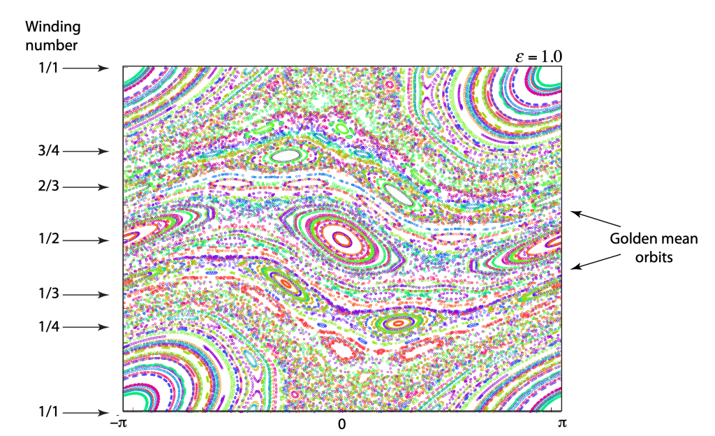
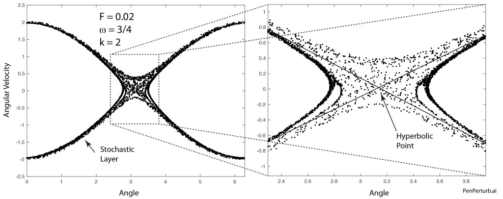
An example of the twist map at strong perturbation ε = 1.0 is shown in Fig. 4. There are numerous island chains. It is easy to find the 1:2 through the 1:7 resonances, but beyond that it is much more difficult to find these rational resonance. Furthermore, there are significant regions of chaotic trajectories associated with the hyperbolic points of the 1:2, 1:3, 1:4 and 1:5 resonances.
Fig. 4. The Standard map at ε = 1.0 slightly above the threshold for the dissolution of the Golde-Mean-Orbit.
In the midst of the island chains and the chaos, there are still continuous (open) orbits that span the phase space without breaks. These are the most irrational numbers–numbers like the golden mean. These are the last orbits to break up. The critical threshold for the breakup of the golden-mean orbit is ε = 0.971. The plot in Fig. 4 is just above that threshold.
All of this behavior of the Standard Map follows from KAM theory, developed by Kolmogorov, Arnold and Moser in the early 1960’s. Although the standard map is specific to the tapped spinning disk, the results and behavior are very general for a wide class of two-dimensional Hamiltonian dynamical systems.
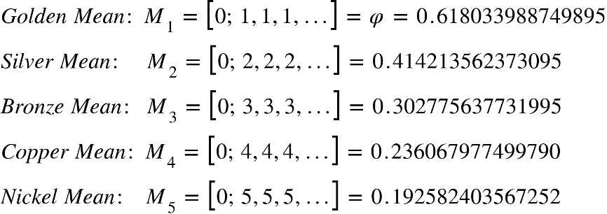
Adiabatic Following: Orbits of the Noble Means
The golden mean is not the only “slowest convergent” among irrational numbers. There are an entire class of irrational numbers whose continued fractions terminate with an infinite series of “1”s. These are known as the “Noble Means”. Examples are:
where the sequence, as q increases to infinity, converges on unity asymptotically among the set of irrationals with the slowest convergents.
There are also the so-called “Metallic Means”, beginning with Gold and moving to Silver, Bronze, Copper, and Nickel. These are:
The challenge for numerical simulations is to find the orbits associated with these Metallic Means for large perturbation parameters ε. One cannot simply pick an initial condition for the Standard Map equal to a Metallic Mean, because at large perturbation, all the orbits have already shifted from their zero-perturbation values.
One of the most important principles in classical mechanics is the concept of adiabatic invariance. All the most common conservation laws of introductory physics–conservation of energy, momentum, and angular momentum–are consequences of adiabatic invariance. Indeed, the phase space of the rigid rotator is ideal for tracking adiabatic invariance because the J-value is the adiabatic invariant. In the numerical simulation, one begins with ε = 0, chooses an initial condition J = φn, and iterates the map as ε slowly increases.
This is shown in the following YouTube video. You will see five special orbits evolve as the perturbation is slowly increased. These are M1 (red), M2 (blue), M3 (green) and two resonances 3:1 (cyan) and 4:1 (magenta). The resonances are expected to break into island chains at relativity low perturbation ε, which is confirmed in the video.
Fig. 5 YouTube video of the Standard Map and special orbits as the perturbation slowly (adiabatically) increases.
Interestingly, the silver mean breaks into a 5:1 island chain around the same perturbation level. This is because the Silver Mean equals 0.414 which approaches 8/5 at moderate perturbation. Therefore, the Silver Mean orbit is “captured” by a 1:5 resonance and remains stable up to very large perturbations approaching ε = 1. The Bronze Mean is captured relativity early into the 1:1 resonance island.
D. D. Nolte, Introduction to Modern Dynamics, 2nd ed. (Oxford University Press, 2019) Link
This Post is Based on Simulations from Chapter 5 of IMD, 2nd edition
This Blog Post is a Companion to the undergraduate physics textbook Modern Dynamics: Chaos, Networks, Space and Time, 2nd ed. (Oxford, 2019) introducing Lagrangians and Hamiltonians, chaos theory, complex systems, synchronization, neural networks, econophysics and Special and General Relativity to Junior and Senior physics majors.
At the dawn of quantum theory, Heisenberg, Schrödinger, Bohr and Pauli were embroiled in a dispute over whether trajectories of particles, defined by their positions over time, could exist. The argument against trajectories was based on an apparent paradox: To draw a “line” depicting a trajectory of a particle along a path implies that there is a momentum vector that carries the particle along that path. But a line is a one-dimensional curve through space, and since at any point in time the particle’s position is perfectly localized, then by Heisenberg’s uncertainty principle, it can have no definable momentum to carry it along.
My previous blog shows the way out of this paradox, by assembling wavepackets that are spread in both space and momentum, explicitly obeying the uncertainty principle. This is nothing new to anyone who has taken a quantum course. But the surprising thing is that in some potentials, like a harmonic potential, the wavepacket travels without broadening, just like classical particles on a trajectory. A dramatic demonstration of this can be seen in this YouTube video. But other potentials “break up” the wavepacket, especially potentials that display classical chaos. Because phase space is one of the best tools for studying classical chaos, especially Hamiltonian chaos, it can be enlisted to dig deeper into the question of the quantum trajectory—not just about the existence of a quantum trajectory, but why quantum systems retain a shadow of their classical counterparts.
Phase Space
Phase space is the state space of Hamiltonian systems. Concepts of phase space were first developed by Boltzmann as he worked on the problem of statistical mechanics. Phase space was later codified by Gibbs for statistical mechanics and by Poincare for orbital mechanics, and it was finally given its name by Paul and Tatiana Ehrenfest (a husband-wife team) in correspondence with the German physicist Paul Hertz (See Chapter 6, “The Tangled Tale of Phase Space”, in Galileo Unbound by D. D. Nolte (Oxford, 2018)).
The stretched-out phase-space functions … are very similar to the stochastic layer that forms in separatrix chaos in classical systems.
The idea of phase space is very simple for classical systems: it is just a plot of the momentum of a particle as a function of its position. For a given initial condition, the trajectory of a particle through its natural configuration space (for instance our 3D world) is traced out as a path through phase space. Because there is one momentum variable per degree of freedom, then the dimensionality of phase space for a particle in 3D is 6D, which is difficult to visualize. But for a one-dimensional dynamical system, like a simple harmonic oscillator (SHO) oscillating in a line, the phase space is just two-dimensional, which is easy to see. The phase-space trajectories of an SHO are simply ellipses, and if the momentum axis is scaled appropriately, the trajectories are circles. The particle trajectory in phase space can be animated just like a trajectory through configuration space as the position and momentum change in time p(x(t)). For the SHO, the point follows the path of a circle going clockwise.
Fig. 1 Phase space of the simple harmonic oscillator. The “orbits” have constant energy.
A more interesting phase space is for the simple pendulum, shown in Fig. 2. There are two types of orbits: open and closed. The closed orbits near the origin are like those of a SHO. The open orbits are when the pendulum is spinning around. The dividing line between the open and closed orbits is called a separatrix. Where the separatrix intersects itself is a saddle point. This saddle point is the most important part of the phase space portrait: it is where chaos emerges when perturbations are added.
Fig. 2 Phase space for a simple pendulum. For small amplitudes the orbits are closed like those of a SHO. For large amplitudes the orbits become open as the pendulum spins about its axis. (Reproduced from Introduction to Modern Dynamics, 2nd Ed., pg. )
One route to classical chaos is through what is known as “separatrix chaos”. It is easy to see why saddle points (also known as hyperbolic points) are the source of chaos: as the system trajectory approaches the saddle, it has two options of which directions to go. Any additional degree of freedom in the system (like a harmonic drive) can make the system go one way on one approach, and the other way on another approach, mixing up the trajectories. An example of the stochastic layer of separatrix chaos is shown in Fig. 3 for a damped driven pendulum. The chaotic behavior that originates at the saddle point extends out along the entire separatrix.
Fig. 3 The stochastic layer of separatrix chaos for a damped driven pendulum. (Reproduced from Introduction to Modern Dynamics, 2nd Ed., pg. )
The main question about whether or not there is a quantum trajectory depends on how quantum packets behave as they approach a saddle point in phase space. Since packets are spread out, it would be reasonable to assume that parts of the packet will go one way, and parts of the packet will go another. But first, one has to ask: Is a phase-space description of quantum systems even possible?
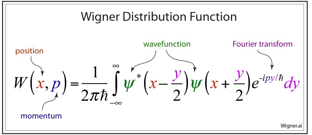
Quantum Phase Space: The Wigner Distribution Function
Phase-space portraits are arguably the most powerful tool in the toolbox of classical dynamics, and one would like to retain its uses for quantum systems. However, there is that pesky paradox about quantum trajectories that cannot admit the existence of one-dimensional curves through such a phase space. Furthermore, there is no direct way of taking a wavefunction and simply “finding” its position or momentum to plot points on such a quantum phase space.
The answer was found in 1932 by Eugene Wigner (1902 – 1905), an Hungarian physicist working at Princeton. He realized that it was impossible to construct a quantum probability distribution in phase space that had positive values everywhere. This is a problem, because negative probabilities have no direct interpretation. But Wigner showed that if one relaxed the requirements a bit, so that expectation values computed over some distribution function (that had positive and negative values) gave correct answers that matched experiments, then this distribution function would “stand in” for an actual probability distribution.
The distribution function that Wigner found is called the Wigner distribution function. Given a wavefunction ψ(x), the Wigner distribution is defined as
Fig. 4 Wigner distribution function in (x, p) phase space.
The Wigner distribution function is the Fourier transform of the convolution of the wavefunction. The pure position dependence of the wavefunction is converted into a spread-out position-momentum function in phase space. For a Gaussian wavefunction ψ(x) with a finite width in space, the W-function in phase space is a two-dimensional Gaussian with finite widths in both space and momentum. In fact, the Δx-Δp product of the W-function is precisely the uncertainty production of the Heisenberg uncertainty relation.
The question of the quantum trajectory from the phase-space perspective becomes whether a Wigner function behaves like a localized “packet” that evolves in phase space in a way analogous to a classical particle, and whether classical chaos is reflected in the behavior of quantum systems.
The Harmonic Oscillator
The quantum harmonic oscillator is a rare and special case among quantum potentials, because the energy spacings between all successive states are all the same. This makes it possible for a Gaussian wavefunction, which is a superposition of the eigenstates of the harmonic oscillator, to propagate through the potential without broadening. To see an example of this, watch the first example in this YouTube video for a Schrödinger cat state in a two-dimensional harmonic potential. For this very special potential, the Wigner distribution behaves just like a (broadened) particle on an orbit in phase space, executing nice circular orbits.
A comparison of the classical phase-space portrait versus the quantum phase-space portrait is shown in Fig. 5. Where the classical particle is a point on an orbit, the quantum particle is spread out, obeying the Δx-Δp Heisenberg product, but following the same orbit as the classical particle.
Fig. 5 Classical versus quantum phase-space portraits for a harmonic oscillator. For a classical particle, the trajectory is a point executing an orbit. For a quantum particle, the trajectory is a Wigner distribution that follows the same orbit as the classical particle.
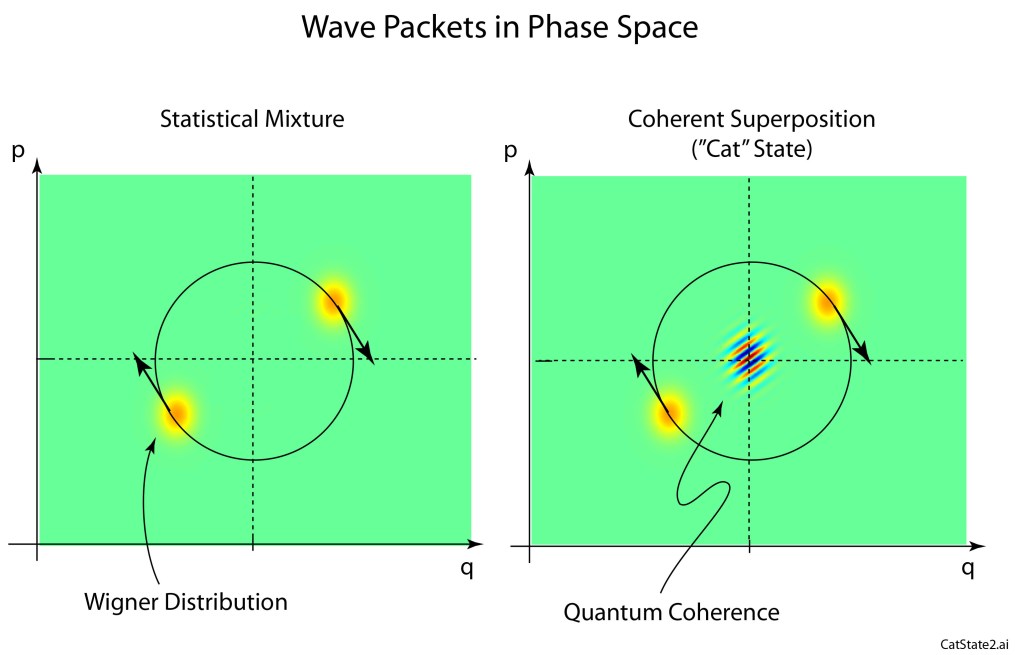
However, a significant new feature appears in the Wigner representation in phase space when there is a coherent superposition of two states, known as a “cat” state, after Schrödinger’s cat. This new feature has no classical analog. It is the coherent interference pattern that appears at the zero-point of the harmonic oscillator for the Schrödinger cat state. There is no such thing as “classical” coherence, so this feature is absent in classical phase space portraits.
Two examples of Wigner distributions are shown in Fig. 6 for a statistical (incoherent) mixture of packets and a coherent superposition of packets. The quantum coherence signature is present in the coherent case but not the statistical mixture case. The coherence in the Wigner distribution represents “off-diagonal” terms in the density matrix that leads to interference effects in quantum systems. Quantum computing algorithms depend critically on such coherences that tend to decay rapidly in real-world physical systems, known as decoherence, and it is possible to make statements about decoherence by watching the zero-point interference.
Fig. 6 Quantum phase-space portraits of double wave packets. On the left, the wave packets have no coherence, being a statistical mixture. On the right is the case for a coherent superposition, or “cat state” for two wave packets in a one-dimensional harmonic oscillator.
Whereas Gaussian wave packets in the quantum harmonic potential behave nearly like classical systems, and their phase-space portraits are almost identical to the classical phase-space view (except for the quantum coherence), most quantum potentials cause wave packets to disperse. And when saddle points are present in the classical case, then we are back to the question about how quantum packets behave as they approach a saddle point in phase space.
Quantum Pendulum and Separatrix Chaos
One of the simplest anharmonic oscillators is the simple pendulum. In the classical case, the period diverges if the pendulum gets very close to going vertical. A similar thing happens in the quantum case, but because the motion has strong anharmonicity, an initial wave packet tends to spread dramatically as parts of the wavefunction less vertical stretch away from the part of the wave function that is more nearly vertical. Fig. 7 is a snap-shot about a eighth of a period after the wave packet was launched. The packet has already stretched out along the separatrix. A double-cat-state was used, so there is a second packet that has coherent interference with the first. To see a movie of the time evolution of the wave packet and the orbit in quantum phase space, see the YouTube video.
Fig. 7 Wavefunction of a quantum pendulum released near vertical. The phase-space portrait is very similar to the classical case, except that the phase-space distribution is stretched out along the separatrix. The initial state for the phase-space portrait was a cat state.
The simple pendulum does have a saddle point, but it is degenerate because the angle is modulo -2-pi. A simple potential that has a non-degenerate saddle point is a double-well potential.
Quantum Double-Well and Separatrix Chaos
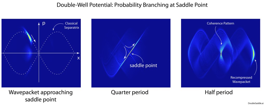
The symmetric double-well potential has a saddle point at the mid-point between the two well minima. A wave packet approaching the saddle will split into to packets that will follow the individual separatrixes that emerge from the saddle point (the unstable manifolds). This effect is seen most dramatically in the middle pane of Fig. 8. For the full video of the quantum phase-space evolution, see this YouTube video. The stretched-out distribution in phase space is highly analogous to the separatrix chaos seen for the classical system.
Fig. 8 Phase-space portraits of the Wigner distribution for a wavepacket in a double-well potential. The packet approaches the central saddle point, where the probability density splits along the unstable manifolds.
Conclusion
A common statement often made about quantum chaos is that quantum systems tend to suppress chaos, only exhibiting chaos for special types of orbits that produce quantum scars. However, from the phase-space perspective, the opposite may be true. The stretched-out Wigner distribution functions, for critical wave packets that interact with a saddle point, are very similar to the stochastic layer that forms in separatrix chaos in classical systems. In this sense, the phase-space description brings out the similarity between classical chaos and quantum chaos.
By David D. Nolte Sept. 25, 2022
YouTube Video
For more on the history of quantum trajectories, see Galileo Unbound from Oxford Press:
Will the next extinction-scale asteroid strike the Earth in our lifetime?
This existential question—the question of our continued existence on this planet—is rhetorical, because there are far too many bodies in our solar system to accurately calculate all trajectories of all asteroids.
The solar system is what is known as an N-body problem. And even the N is not well determined. The asteroid belt alone has over a million extinction-sized asteroids, and there are tens of millions of smaller ones that could still do major damage to life on Earth if they hit. To have a hope of calculating even one asteroid trajectory do we ignore planetary masses that are too small? What is too small? What if we only consider the Sun, the Earth and Jupiter? This is what Euler did in 1760, and he still had to make more assumptions.
Stability of the Solar System
Once Newton published his Principia, there was a pressing need to calculate the orbit of the Moon (see my blog post on the three-body problem). This was important for navigation, because if the daily position of the moon could be known with sufficient accuracy, then ships would have a means to determine their longitude at sea. However, the Moon, Earth and Sun are already a three-body problem, which still ignores the effects of Mars and Jupiter on the Moon’s orbit, not to mention the problem that the Earth is not a perfect sphere. Therefore, to have any hope of success, toy systems that were stripped of all their obfuscating detail were needed.
Euler investigated simplified versions of the three-body problem around 1760, treating a body attracted to two fixed centers of gravity moving in the plane, and he solved it using elliptic integrals. When the two fixed centers are viewed in a coordinate frame that is rotating with the Sun-Earth system, it can come close to capturing many of the important details of the system. In 1762 Euler tried another approach, called the restricted three-body problem, where he considered a massless Moon attracted to a massive Earth orbiting a massive Sun, again all in the plane. Euler could not find general solutions to this problem, but he did stumble on an interesting special case when the three bodies remain collinear throughout their motions in a rotating reference frame.
It was not the danger of asteroids that was the main topic of interest in those days, but the question whether the Earth itself is in a stable orbit and is safe from being ejected from the Solar system. Despite steadily improving methods for calculating astronomical trajectories through the nineteenth century, this question of stability remained open.
Poincaré and the King Oscar Prize of 1889
Some years ago I wrote an article for Physics Today called “The Tangled Tale of Phase Space” that tracks the historical development of phase space. One of the chief players in that story was Henri Poincaré (1854 – 1912). Henri Poincare was the Einstein before Einstein. He was a minor celebrity and was considered to be the greatest genius of his era. The event in his early career that helped launch him to stardom was a mathematics prize announced in 1887 to honor the birthday of King Oscar II of Sweden. The challenge problem was as simple as it was profound: Prove rigorously whether the solar system is stable.
This was the old N-body problem that had so far resisted solution, but there was a sense at that time that recent mathematical advances might make the proof possible. There was even a rumor that Dirichlet had outlined such a proof, but no trace of the outline could be found in his papers after his death in 1859.
The prize competition was announced in Acta Mathematica, written by the Swedish mathematician Gösta Mittag-Leffler. It stated:
Given a system of arbitrarily many mass points that attract each according to Newton’s law, under the assumption that no two points ever collide, try to find a representation of the coordinates of each point as a series in a variable that is some known function of time and for all of whose values the series converges uniformly.
The timing of the prize was perfect for Poincaré who was in his early thirties and just beginning to make his mark on mathematics. He was working on the theory of dynamical systems and was developing a new viewpoint that went beyond integrating single trajectories by focusing more broadly on whole classes of solutions. The question of the stability of the solar system seemed like a good problem to use to sharpen his mathematical tools. The general problem was still too difficult, so he began with Euler’s restricted three-body problem. He made steady progress, and along the way he invented an array of new techniques for studying the general properties of dynamical systems. One of these was the Poincaré section. Another was his set of integral invariants, one of which is recognized as the conservation of volume in phase space, also known as Liouville’s theorem, although it was Ludwig Boltzmann who first derived this result (see my Physics Today article). Eventually, he believed he had proven that the restricted three-body problem was stable.
By the time Poincaré had finished is prize submission, he had invented a new field of mathematical analysis, and the judges of the prize submission recognized it. Poincaré was named the winner, and his submission was prepared for publication in the Acta. However, Mittag-Leffler was a little concerned by a technical objection that had been raised, so he forwarded the comment to Poincaré for him to look at. At first, Poincaré thought the objection could easily be overcome, but as he worked on it and delved deeper, he had a sudden attack of panic. Trajectories near a saddle point did not converge. His proof of stability was wrong!
He alerted Mittag-Leffler to stop the presses, but it was too late. The first printing had been completed and review copies had already been sent to the judges. Mittag-Leffler immediately wrote to them asking for their return while Poincaré worked nonstop to produce a corrected copy. When he had completed his reanalysis, he had discovered a divergent feature of the solution to the dynamical problem near saddle points that is recognized today as the discovery of chaos. Poincaré paid for the reprinting of his paper out of his own pocket and (almost) all of the original printing was destroyed. This embarrassing moment in the life of a great mathematician was virtually forgotten until it was brought to light by the historian Barrow-Green in 1994 [1].
Poincaré is still a popular icon in France. Here is the Poincaré cafe in Paris.
A crater on the Moon is named after Poincaré.
Chaos in the Poincaré Return Map
Despite the fact that his conclusions on the stability of the 3-body problem flipped, Poincaré’s new tools for analyzing dynamical systems earned him the prize. He did not stop at his modified prize submission but continued working on systematizing his methods, publishing New Methods in Celestial Mechanics in several volumes through the 1890’s. It was here that he fully explored what happens when a trajectory approaches a saddle point of dynamical equilibrium.
The third volume of a three-book series that grew from Poincaré’s award-winning paper
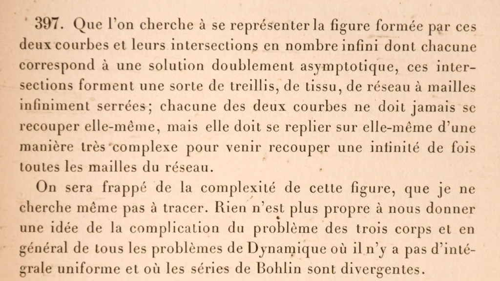
To visualize a periodic trajectory, Poincaré invented a mathematical tool called a “first-return map”, also known as a Poincaré section. It was a way of taking a higher dimensional continuous trajectory and turning it into a simple iterated discrete map. Therefore, one did not need to solve continuous differential equations, it was enough to just iterate the map. In this way, complicated periodic, or nearly periodic, behavior could be explored numerically. However, even armed with this weapon, Poincaré found that iterated maps became unstable as a trajectory that originated from a saddle point approached another equivalent saddle point. Because the dynamics are periodic, the outgoing and incoming trajectories are opposite ends of the same trajectory, repeated with 2-pi periodicity. Therefore, the saddle point is also called a homoclinic point, meaning that trajectories in the discrete map intersect with themselves. (If two different trajectories in the map intersect, that is called a heteroclinic point.) When Poincaré calculated the iterations around the homoclinic point, he discovered a wild and complicated pattern in which a trajectory intersected itself many times. Poincaré wrote:
[I]f one seeks to visualize the pattern formed by these two curves and their infinite number of intersections … these intersections form a kind of lattice work, a weave, a chain-link network of infinitely fine mesh; each of the two curves can never cross itself, but it must fold back on itself in a very complicated way so as to recross all the chain-links an infinite number of times .… One will be struck by the complexity of this figure, which I am not even attempting to draw. Nothing can give us a better idea of the intricacy of the three-body problem, and of all the problems of dynamics in general…
Poincaré’s first view of chaos.
This was the discovery of chaos! Today we call this “lattice work” the “homoclinic tangle”. He could not draw it with the tools of his day … but we can!
Chirikov’s Standard Map
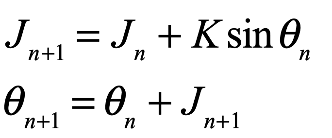
The restricted 3-body problem is a bit more complicated than is needed to illustrate Poincaré’s homoclinic tangle. A much simpler model is a discrete map called Chirikov’s Map or the Standard Map. It describes the Poincaré section of a periodically kicked oscillator that rotates or oscillates in the angular direction with an angular momentm J. The map has the simple form
in which the angular momentum in updated first, and then the angle variable is updated with the new angular momentum. When plotted on the (θ,J) plane, the standard map produces a beautiful kaleidograph of intertwined trajectories piercing the Poincaré plane, as shown in the figure below. The small points or dots are successive intersections of the higher-dimensional trajectory intersecting a plane. It is possible to trace successive points by starting very close to a saddle point (on the left) and connecting successive iterates with lines. These lines merge into the black trace in the figure that emerges along the unstable manifold of the saddle point on the left and approaches the saddle point on the right generally along the stable manifold.
Fig. Standard map for K = 0.97 at the transition to full chaos. The dark line is the trajectory of the unstable manifold emerging from the saddle point at (p,0). Note the wild oscillations as it approaches the saddle point at (3pi,0).
However, as the successive iterates approach the new saddle (which is really just the old saddle point because of periodicity) it crosses the stable manifold again and again, in ever wilder swings that diverge as it approaches the saddle point. This is just one trace. By calculating traces along all four stable and unstable manifolds and carrying them through to the saddle, a lattice work, or homoclinic tangle emerges.
Two of those traces originate from the stable manifolds, so to calculate their contributions to the homoclinic tangle, one must run these traces backwards in time using the inverse Chirikov map. This is
The four traces all intertwine at the saddle point in the figure below with a zoom in on the tangle in the next figure. This is the lattice work that Poincaré glimpsed in 1889 as he worked feverishly to correct the manuscript that won him the prize that established him as one of the preeminent mathematicians of Europe.
Fig. The homoclinic tangle caused by the folding of phase space trajectories as stable and unstable manifolds criss-cross in the Poincare map at the saddle point. This was the figure that Poincaré could not attempt to draw because of its complexity.
Fig. A zoom-in of the homoclinic tangle at the saddle point as the stable and unstable manifolds create a lattice of intersections. This is the fundamental origin of chaos and the sensitivity to initial conditions (SIC) that make forecasting almost impossible in chaotic systems.
The Path from Galileo’s Trajectory to Complex Systems and Quantum Science.
Read more about the history of chaos theory in Galileo Unbound from Oxford University Press
[6] Poincaré H and Goroff DL. New methods of celestial mechanics … Edited and introduced by Daniel L. Goroff. New York: American Institute of Physics, 1993.
It is surprising how much of modern dynamics boils down to an extremely simple formula
This innocuous-looking equation carries such riddles, such surprises, such unintuitive behavior that it can become the object of study for life. This equation is called a vector flow equation, and it can be used to capture the essential physics of economies, neurons, ecosystems, networks, and even orbits of photons around black holes. This equation is to modern dynamics what F = ma was to classical mechanics. It is the starting point for understanding complex systems.
The Magic of Phase Space
The apparent simplicity of the “flow equation” masks the complexity it contains. It is a vector equation because each “dimension” is a variable of a complex system. Many systems of interest may have only a few variables, but ecosystems and economies and social networks may have hundreds or thousands of variables. Expressed in component format, the flow equation is
where the superscript spans the number of variables. But even this masks all that can happen with such an equation. Each of the functions fa can be entirely different from each other, and can be any type of function, whether polynomial, rational, algebraic, transcendental or composite, although they must be single-valued. They are generally nonlinear, and the limitless ways that functions can be nonlinear is where the richness of the flow equation comes from.
The vector flow equation is an ordinary differential equation (ODE) that can be solved for specific trajectories as initial value problems. A single set of initial conditions defines a unique trajectory. For instance, the trajectory for a 4-dimensional example is described as the column vector
which is the single-parameter position vector to a point in phase space, also called state space. The point sweeps through successive configurations as a function of its single parameter—time. This trajectory is also called an orbit. In classical mechanics, the focus has tended to be on the behavior of specific orbits that arise from a specific set of initial conditions. This is the classic “rock thrown from a cliff” problem of introductory physics courses. However, in modern dynamics, the focus shifts away from individual trajectories to encompass the set of all possible trajectories.
Why is Modern Dynamics part of Physics?
If finding the solutions to the “x-dot equals f” vector flow equation is all there is to do, then this would just be a math problem—the solution of ODE’s. There are plenty of gems for mathematicians to look for, and there is an entire of field of study in mathematics called “dynamical systems“, but this would not be “physics”. Physics as a profession is separate and distinct from mathematics, although the two are sometimes confused. Physics uses mathematics as its language and as its toolbox, but physics is not mathematics. Physics is done best when it is done qualitatively—this means with scribbles done on napkins in restaurants or on the back of envelopes while waiting in line. Physics is about recognizing relationships and patterns. Physics is about identifying the limits to scaling properties where the physics changes when scales change. Physics is about the mapping of the simplest possible mathematics onto behavior in the physical world, and recognizing when the simplest possible mathematics is a universal that applies broadly to diverse systems that seem different, but that share the same underlying principles.
So, granted solving ODE’s is not physics, there is still a tremendous amount of good physics that can be done by solving ODE’s. ODE solvers become the modern physicist’s experimental workbench, providing data output from numerical experiments that can test the dependence on parameters in ways that real-world experiments might not be able to access. Physical intuition can be built based on such simulations as the engaged physicist begins to “understand” how the system behaves, able to explain what will happen as the values of parameters are changed.
In the follow sections, three examples of modern dynamics are introduced with a preliminary study, including Python code. These examples are: Galactic dynamics, synchronized networks and ecosystems. Despite their very different natures, their description using dynamical flows share features in common and illustrate the beauty and depth of behavior that can be explored with simple equations.
Galactic Dynamics
One example of the power and beauty of the vector flow equation and its set of all solutions in phase space is called the Henon-Heiles model of the motion of a star within a galaxy. Of course, this is a terribly complicated problem that involves tens of billions of stars, but if you average over the gravitational potential of all the other stars, and throw in a couple of conservation laws, the resulting potential can look surprisingly simple. The motion in the plane of this galactic potential takes two configuration coordinates (x, y) with two associated momenta (px, py) for a total of four dimensions. The flow equations in four-dimensional phase space are simply
Fig. 1 The 4-dimensional phase space flow equations of a star in a galaxy. The terms in light blue are a simple two-dimensional harmonic oscillator. The terms in magenta are the nonlinear contributions from the stars in the galaxy.
where the terms in the light blue box describe a two-dimensional simple harmonic oscillator (SHO), which is a linear oscillator, modified by the terms in the magenta box that represent the nonlinear galactic potential. The orbits of this Hamiltonian system are chaotic, and because there is no dissipation in the model, a single orbit will continue forever within certain ranges of phase space governed by energy conservation, but never quite repeating.
Fig. 2 Two-dimensional Poincaré section of sets of trajectories in four-dimensional phase space for the Henon-Heiles galactic dynamics model. The perturbation parameter is &eps; = 0.3411 and the energy E = 1.
#!/usr/bin/env python3
# -*- coding: utf-8 -*-
"""
Hamilton4D.py
Created on Wed Apr 18 06:03:32 2018

@author: nolte

Derived from:
D. D. Nolte, Introduction to Modern Dynamics: Chaos, Networks, Space and Time, 2nd ed. (Oxford,2019)
"""

import numpy as np
import matplotlib as mpl
from mpl_toolkits.mplot3d import Axes3D
from scipy import integrate
from matplotlib import pyplot as plt
from matplotlib import cm
import time
import os

plt.close('all')

# model_case 1 = Heiles
# model_case 2 = Crescent
print(' ')
print('Hamilton4D.py')
print('Case: 1 = Heiles')
print('Case: 2 = Crescent')
model_case = int(input('Enter the Model Case (1-2)'))

if model_case == 1:
    E = 1       # Heiles: 1, 0.3411   Crescent: 0.05, 1
    epsE = 0.3411   # 3411
    def flow_deriv(x_y_z_w,tspan):
        x, y, z, w = x_y_z_w
        a = z
        b = w
        c = -x - epsE*(2*x*y)
        d = -y - epsE*(x**2 - y**2)
        return[a,b,c,d]
else:
    E = .1       #   Crescent: 0.1, 1
    epsE = 1
    def flow_deriv(x_y_z_w,tspan):
        x, y, z, w = x_y_z_w
        a = z
        b = w
        c = -(epsE*(y-2*x**2)*(-4*x) + x)
        d = -(y-epsE*2*x**2)
        return[a,b,c,d]

prms = np.sqrt(E)
pmax = np.sqrt(2*E)

# Potential Function
if model_case == 1:
    V = np.zeros(shape=(100,100))
    for xloop in range(100):
        x = -2 + 4*xloop/100
        for yloop in range(100):
            y = -2 + 4*yloop/100
            V[yloop,xloop] = 0.5*x**2 + 0.5*y**2 + epsE*(x**2*y - 0.33333*y**3)
else:
    V = np.zeros(shape=(100,100))
    for xloop in range(100):
        x = -2 + 4*xloop/100
        for yloop in range(100):
            y = -2 + 4*yloop/100
            V[yloop,xloop] = 0.5*x**2 + 0.5*y**2 + epsE*(2*x**4 - 2*x**2*y)

fig = plt.figure(1)
contr = plt.contourf(V,100, cmap=cm.coolwarm, vmin = 0, vmax = 10)
fig.colorbar(contr, shrink=0.5, aspect=5)
fig = plt.show()

repnum = 250
mulnum = 64/repnum

np.random.seed(1)
for reploop  in range(repnum):
    px1 = 2*(np.random.random((1))-0.499)*pmax
    py1 = np.sign(np.random.random((1))-0.499)*np.real(np.sqrt(2*(E-px1**2/2)))
    xp1 = 0
    yp1 = 0

    x_y_z_w0 = [xp1, yp1, px1, py1]

    tspan = np.linspace(1,1000,10000)
    x_t = integrate.odeint(flow_deriv, x_y_z_w0, tspan)
    siztmp = np.shape(x_t)
    siz = siztmp[0]

    if reploop % 50 == 0:
        plt.figure(2)
        lines = plt.plot(x_t[:,0],x_t[:,1])
        plt.setp(lines, linewidth=0.5)
        plt.show()
        time.sleep(0.1)
        #os.system("pause")

    y1 = x_t[:,0]
    y2 = x_t[:,1]
    y3 = x_t[:,2]
    y4 = x_t[:,3]

    py = np.zeros(shape=(2*repnum,))
    yvar = np.zeros(shape=(2*repnum,))
    cnt = -1
    last = y1[1]
    for loop in range(2,siz):
        if (last < 0)and(y1[loop] > 0):
            cnt = cnt+1
            del1 = -y1[loop-1]/(y1[loop] - y1[loop-1])
            py[cnt] = y4[loop-1] + del1*(y4[loop]-y4[loop-1])
            yvar[cnt] = y2[loop-1] + del1*(y2[loop]-y2[loop-1])
            last = y1[loop]
        else:
            last = y1[loop]

    plt.figure(3)
    lines = plt.plot(yvar,py,'o',ms=1)
    plt.show()

if model_case == 1:
    plt.savefig('Heiles')
else:
    plt.savefig('Crescent')
Networks, Synchronization and Emergence
A central paradigm of nonlinear science is the emergence of patterns and organized behavior from seemingly random interactions among underlying constituents. Emergent phenomena are among the most awe inspiring topics in science. Crystals are emergent, forming slowly from solutions of reagents. Life is emergent, arising out of the chaotic soup of organic molecules on Earth (or on some distant planet). Intelligence is emergent, and so is consciousness, arising from the interactions among billions of neurons. Ecosystems are emergent, based on competition and symbiosis among species. Economies are emergent, based on the transfer of goods and money spanning scales from the local bodega to the global economy.
One of the common underlying properties of emergence is the existence of networks of interactions. Networks and network science are topics of great current interest driven by the rise of the World Wide Web and social networks. But networks are ubiquitous and have long been the topic of research into complex and nonlinear systems. Networks provide a scaffold for understanding many of the emergent systems. It allows one to think of isolated elements, like molecules or neurons, that interact with many others, like the neighbors in a crystal or distant synaptic connections.
From the point of view of modern dynamics, the state of a node can be a variable or a “dimension” and the interactions among links define the functions of the vector flow equation. Emergence is then something that “emerges” from the dynamical flow as many elements interact through complex networks to produce simple or emergent patterns.
Synchronization is a form of emergence that happens when lots of independent oscillators, each vibrating at their own personal frequency, are coupled together to push and pull on each other, entraining all the individual frequencies into one common global oscillation of the entire system. Synchronization plays an important role in the solar system, explaining why the Moon always shows one face to the Earth, why Saturn’s rings have gaps, and why asteroids are mainly kept away from colliding with the Earth. Synchronization plays an even more important function in biology where it coordinates the beating of the heart and the functioning of the brain.
One of the most dramatic examples of synchronization is the Kuramoto synchronization phase transition. This occurs when a large set of individual oscillators with differing natural frequencies interact with each other through a weak nonlinear coupling. For small coupling, all the individual nodes oscillate at their own frequency. But as the coupling increases, there is a sudden coalescence of all the frequencies into a single common frequency. This mechanical phase transition, called the Kuramoto transition, has many of the properties of a thermodynamic phase transition, including a solution that utilizes mean field theory.
Fig. 3 The Kuramoto model for the nonlinear coupling of N simple phase oscillators. The term in light blue is the simple phase oscillator. The term in magenta is the global nonlinear coupling that connects each oscillator to every other.
The simulation of 20 Poncaré phase oscillators with global coupling is shown in Fig. 4 as a function of increasing coupling coefficient g. The original individual frequencies are spread randomly. The oscillators with similar frequencies are the first to synchronize, forming small clumps that then synchronize with other clumps of oscillators, until all oscillators are entrained to a single compromise frequency. The Kuramoto phase transition is not sharp in this case because the value of N = 20 is too small. If the simulation is run for 200 oscillators, there is a sudden transition from unsynchronized to synchronized oscillation at a threshold value of g.
Fig. 4 The Kuramoto model for 20 Poincare oscillators showing the frequencies as a function of the coupling coefficient.
The Kuramoto phase transition is one of the most important fundamental examples of modern dynamics because it illustrates many facets of nonlinear dynamics in a very simple way. It highlights the importance of nonlinearity, the simplification of phase oscillators, the use of mean field theory, the underlying structure of the network, and the example of a mechanical analog to a thermodynamic phase transition. It also has analytical solutions because of its simplicity, while still capturing the intrinsic complexity of nonlinear systems.
#!/usr/bin/env python3
# -*- coding: utf-8 -*-
"""
Created on Sat May 11 08:56:41 2019

@author: nolte

D. D. Nolte, Introduction to Modern Dynamics: Chaos, Networks, Space and Time, 2nd ed. (Oxford,2019)
"""

# https://www.python-course.eu/networkx.php
# https://networkx.github.io/documentation/stable/tutorial.html
# https://networkx.github.io/documentation/stable/reference/functions.html

import numpy as np
from scipy import integrate
from matplotlib import pyplot as plt
import networkx as nx
from UserFunction import linfit
import time

tstart = time.time()

plt.close('all')

Nfac = 25   # 25
N = 50      # 50
width = 0.2

# model_case 1 = complete graph (Kuramoto transition)
# model_case 2 = Erdos-Renyi
model_case = int(input('Input Model Case (1-2)'))
if model_case == 1:
    facoef = 0.2
    nodecouple = nx.complete_graph(N)
elif model_case == 2:
    facoef = 5
    nodecouple = nx.erdos_renyi_graph(N,0.1)


# function: omegout, yout = coupleN(G)
def coupleN(G):

    # function: yd = flow_deriv(x_y)
    def flow_deriv(y,t0):

        yp = np.zeros(shape=(N,))
        for omloop  in range(N):
            temp = omega[omloop]
            linksz = G.node[omloop]['numlink']
            for cloop in range(linksz):
                cindex = G.node[omloop]['link'][cloop]
                g = G.node[omloop]['coupling'][cloop]

                temp = temp + g*np.sin(y[cindex]-y[omloop])

            yp[omloop] = temp

        yd = np.zeros(shape=(N,))
        for omloop in range(N):
            yd[omloop] = yp[omloop]

        return yd
    # end of function flow_deriv(x_y)

    mnomega = 1.0

    for nodeloop in range(N):
        omega[nodeloop] = G.node[nodeloop]['element']

    x_y_z = omega

    # Settle-down Solve for the trajectories
    tsettle = 100
    t = np.linspace(0, tsettle, tsettle)
    x_t = integrate.odeint(flow_deriv, x_y_z, t)
    x0 = x_t[tsettle-1,0:N]

    t = np.linspace(1,1000,1000)
    y = integrate.odeint(flow_deriv, x0, t)
    siztmp = np.shape(y)
    sy = siztmp[0]

    # Fit the frequency
    m = np.zeros(shape = (N,))
    w = np.zeros(shape = (N,))
    mtmp = np.zeros(shape=(4,))
    btmp = np.zeros(shape=(4,))
    for omloop in range(N):

        if np.remainder(sy,4) == 0:
            mtmp[0],btmp[0] = linfit(t[0:sy//2],y[0:sy//2,omloop]);
            mtmp[1],btmp[1] = linfit(t[sy//2+1:sy],y[sy//2+1:sy,omloop]);
            mtmp[2],btmp[2] = linfit(t[sy//4+1:3*sy//4],y[sy//4+1:3*sy//4,omloop]);
            mtmp[3],btmp[3] = linfit(t,y[:,omloop]);
        else:
            sytmp = 4*np.floor(sy/4);
            mtmp[0],btmp[0] = linfit(t[0:sytmp//2],y[0:sytmp//2,omloop]);
            mtmp[1],btmp[1] = linfit(t[sytmp//2+1:sytmp],y[sytmp//2+1:sytmp,omloop]);
            mtmp[2],btmp[2] = linfit(t[sytmp//4+1:3*sytmp/4],y[sytmp//4+1:3*sytmp//4,omloop]);
            mtmp[3],btmp[3] = linfit(t[0:sytmp],y[0:sytmp,omloop]);


        #m[omloop] = np.median(mtmp)
        m[omloop] = np.mean(mtmp)

        w[omloop] = mnomega + m[omloop]

    omegout = m
    yout = y

    return omegout, yout
    # end of function: omegout, yout = coupleN(G)


Nlink = N*(N-1)//2
omega = np.zeros(shape=(N,))
omegatemp = width*(np.random.rand(N)-1)
meanomega = np.mean(omegatemp)
omega = omegatemp - meanomega
sto = np.std(omega)

lnk = np.zeros(shape = (N,), dtype=int)
for loop in range(N):
    nodecouple.node[loop]['element'] = omega[loop]
    nodecouple.node[loop]['link'] = list(nx.neighbors(nodecouple,loop))
    nodecouple.node[loop]['numlink'] = np.size(list(nx.neighbors(nodecouple,loop)))
    lnk[loop] = np.size(list(nx.neighbors(nodecouple,loop)))

avgdegree = np.mean(lnk)
mnomega = 1

facval = np.zeros(shape = (Nfac,))
yy = np.zeros(shape=(Nfac,N))
xx = np.zeros(shape=(Nfac,))
for facloop in range(Nfac):
    print(facloop)

    fac = facoef*(16*facloop/(Nfac))*(1/(N-1))*sto/mnomega
    for nodeloop in range(N):
        nodecouple.node[nodeloop]['coupling'] = np.zeros(shape=(lnk[nodeloop],))
        for linkloop in range (lnk[nodeloop]):
            nodecouple.node[nodeloop]['coupling'][linkloop] = fac

    facval[facloop] = fac*avgdegree

    omegout, yout = coupleN(nodecouple)                           # Here is the subfunction call for the flow

    for omloop in range(N):
        yy[facloop,omloop] = omegout[omloop]

    xx[facloop] = facval[facloop]

plt.figure(1)
lines = plt.plot(xx,yy)
plt.setp(lines, linewidth=0.5)
plt.show()

elapsed_time = time.time() - tstart
print('elapsed time = ',format(elapsed_time,'.2f'),'secs')
The Web of Life
Ecosystems are among the most complex systems on Earth. The complex interactions among hundreds or thousands of species may lead to steady homeostasis in some cases, to growth and collapse in other cases, and to oscillations or chaos in yet others. But the definition of species can be broad and abstract, referring to businesses and markets in economic ecosystems, or to cliches and acquaintances in social ecosystems, among many other examples. These systems are governed by the laws of evolutionary dynamics that include fitness and survival as well as adaptation.
The dimensionality of the dynamical spaces for these systems extends to hundreds or thousands of dimensions—far too complex to visualize when thinking in four dimensions is already challenging. Yet there are shared principles and common behaviors that emerge even here. Many of these can be illustrated in a simple three-dimensional system that is represented by a triangular simplex that can be easily visualized, and then generalized back to ultra-high dimensions once they are understood.
A simplex is a closed (N-1)-dimensional geometric figure that describes a zero-sum game (game theory is an integral part of evolutionary dynamics) among N competing species. For instance, a two-simplex is a triangle that captures the dynamics among three species. Each vertex of the triangle represents the situation when the entire ecosystem is composed of a single species. Anywhere inside the triangle represents the situation when all three species are present and interacting.
A classic model of interacting species is the replicator equation. It allows for a fitness-based proliferation and for trade-offs among the individual species. The replicator dynamics equations are shown in Fig. 5.
Fig. 5 Replicator dynamics has a surprisingly simple form, but with surprisingly complicated behavior. The key elements are the fitness and the payoff matrix. The fitness relates to how likely the species will survive. The payoff matrix describes how one species gains at the loss of another (although symbiotic relationships also occur).
The population dynamics on the 2D simplex are shown in Fig. 6 for several different pay-off matrices. The matrix values are shown in color and help interpret the trajectories. For instance the simplex on the upper-right shows a fixed point center. This reflects the antisymmetric character of the pay-off matrix around the diagonal. The stable spiral on the lower-left has a nearly asymmetric pay-off matrix, but with unequal off-diagonal magnitudes. The other two cases show central saddle points with stable fixed points on the boundary. A very large variety of behaviors are possible for this very simple system. The Python program is shown in Trirep.py.
Fig. 6 Payoff matrix and population simplex for four random cases: Upper left is an unstable saddle. Upper right is a center. Lower left is a stable spiral. Lower right is a marginal case.
#!/usr/bin/env python3
# -*- coding: utf-8 -*-
"""
trirep.py
Created on Thu May  9 16:23:30 2019

@author: nolte

Derived from:
D. D. Nolte, Introduction to Modern Dynamics: Chaos, Networks, Space and Time, 2nd ed. (Oxford,2019)
"""

import numpy as np
from scipy import integrate
from matplotlib import pyplot as plt

plt.close('all')

def tripartite(x,y,z):

    sm = x + y + z
    xp = x/sm
    yp = y/sm

    f = np.sqrt(3)/2

    y0 = f*xp
    x0 = -0.5*xp - yp + 1;

    plt.figure(2)
    lines = plt.plot(x0,y0)
    plt.setp(lines, linewidth=0.5)
    plt.plot([0, 1],[0, 0],'k',linewidth=1)
    plt.plot([0, 0.5],[0, f],'k',linewidth=1)
    plt.plot([1, 0.5],[0, f],'k',linewidth=1)
    plt.show()


def solve_flow(y,tspan):
    def flow_deriv(y, t0):
    #"""Compute the time-derivative ."""

        f = np.zeros(shape=(N,))
        for iloop in range(N):
            ftemp = 0
            for jloop in range(N):
                ftemp = ftemp + A[iloop,jloop]*y[jloop]
            f[iloop] = ftemp

        phitemp = phi0          # Can adjust this from 0 to 1 to stabilize (but Nth population is no longer independent)
        for loop in range(N):
            phitemp = phitemp + f[loop]*y[loop]
        phi = phitemp

        yd = np.zeros(shape=(N,))
        for loop in range(N-1):
            yd[loop] = y[loop]*(f[loop] - phi);

        if np.abs(phi0) < 0.01:             # average fitness maintained at zero
            yd[N-1] = y[N-1]*(f[N-1]-phi);
        else:                                     # non-zero average fitness
            ydtemp = 0
            for loop in range(N-1):
                ydtemp = ydtemp - yd[loop]
            yd[N-1] = ydtemp

        return yd

    # Solve for the trajectories
    t = np.linspace(0, tspan, 701)
    x_t = integrate.odeint(flow_deriv,y,t)
    return t, x_t

# model_case 1 = zero diagonal
# model_case 2 = zero trace
# model_case 3 = asymmetric (zero trace)
print(' ')
print('trirep.py')
print('Case: 1 = antisymm zero diagonal')
print('Case: 2 = antisymm zero trace')
print('Case: 3 = random')
model_case = int(input('Enter the Model Case (1-3)'))

N = 3
asymm = 3      # 1 = zero diag (replicator eqn)   2 = zero trace (autocatylitic model)  3 = random (but zero trace)
phi0 = 0.001            # average fitness (positive number) damps oscillations
T = 100;


if model_case == 1:
    Atemp = np.zeros(shape=(N,N))
    for yloop in range(N):
        for xloop in range(yloop+1,N):
            Atemp[yloop,xloop] = 2*(0.5 - np.random.random(1))
            Atemp[xloop,yloop] = -Atemp[yloop,xloop]

if model_case == 2:
    Atemp = np.zeros(shape=(N,N))
    for yloop in range(N):
        for xloop in range(yloop+1,N):
            Atemp[yloop,xloop] = 2*(0.5 - np.random.random(1))
            Atemp[xloop,yloop] = -Atemp[yloop,xloop]
        Atemp[yloop,yloop] = 2*(0.5 - np.random.random(1))
    tr = np.trace(Atemp)
    A = Atemp
    for yloop in range(N):
        A[yloop,yloop] = Atemp[yloop,yloop] - tr/N

else:
    Atemp = np.zeros(shape=(N,N))
    for yloop in range(N):
        for xloop in range(N):
            Atemp[yloop,xloop] = 2*(0.5 - np.random.random(1))

    tr = np.trace(Atemp)
    A = Atemp
    for yloop in range(N):
        A[yloop,yloop] = Atemp[yloop,yloop] - tr/N

plt.figure(3)
im = plt.matshow(A,3,cmap=plt.cm.get_cmap('seismic'))  # hsv, seismic, bwr
cbar = im.figure.colorbar(im)

M = 20
delt = 1/M
ep = 0.01;

tempx = np.zeros(shape = (3,))
for xloop in range(M):
    tempx[0] = delt*(xloop)+ep;
    for yloop in range(M-xloop):
        tempx[1] = delt*yloop+ep
        tempx[2] = 1 - tempx[0] - tempx[1]

        x0 = tempx/np.sum(tempx);          # initial populations

        tspan = 70
        t, x_t = solve_flow(x0,tspan)

        y1 = x_t[:,0]
        y2 = x_t[:,1]
        y3 = x_t[:,2]

        plt.figure(1)
        lines = plt.plot(t,y1,t,y2,t,y3)
        plt.setp(lines, linewidth=0.5)
        plt.show()
        plt.ylabel('X Position')
        plt.xlabel('Time')

        tripartite(y1,y2,y3)
Topics in Modern Dynamics
These three examples are just the tip of the iceberg. The topics in modern dynamics are almost numberless. Any system that changes in time is a potential object of study in modern dynamics. Here is a list of a few topics that spring to mind.
Hamiltonian systems are freaks of nature. Unlike the everyday world we experience that is full of dissipation and inefficiency, Hamiltonian systems live in a world free of loss. Despite how rare this situation is for us, this unnatural state happens commonly in two extremes: orbital mechanics and quantum mechanics. In the case of orbital mechanics, dissipation does exist, most commonly in tidal effects, but effects of dissipation in the orbits of moons and planets takes eons to accumulate, making these systems effectively free of dissipation on shorter time scales. Quantum mechanics is strictly free of dissipation, but there is a strong caveat: ALL quantum states need to be included in the quantum description. This includes the coupling of discrete quantum states to their environment. Although it is possible to isolate quantum systems to a large degree, it is never possible to isolate them completely, and they do interact with the quantum states of their environment, if even just the black-body radiation from their container, and even if that container is cooled to milliKelvins. Such interactions involve so many degrees of freedom, that it all behaves like dissipation. The origin of quantum decoherence, which poses such a challenge for practical quantum computers, is the entanglement of quantum systems with their environment.
Liouville’s theorem plays a central role in the explanation of the entropy and ergodic properties of ideal gases, as well as in Hamiltonian chaos.
Liouville’s Theorem and Phase Space
A middle ground of practically ideal Hamiltonian mechanics can be found in the dynamics of ideal gases. This is the arena where Maxwell and Boltzmann first developed their theories of statistical mechanics using Hamiltonian physics to describe the large numbers of particles. Boltzmann applied a result he learned from Jacobi’s Principle of the Last Multiplier to show that a volume of phase space is conserved despite the large number of degrees of freedom and the large number of collisions that take place. This was the first derivation of what is today known as Liouville’s theorem.
Close-up of the Lozi Map with B = -1 and C = 0.5.
In 1838 Joseph Liouville, a pure mathematician, was interested in classes of solutions of differential equations. In a short paper, he showed that for one class of differential equation one could define a property that remained invariant under the time evolution of the system. This purely mathematical paper by Liouville was expanded upon by Jacobi, who was a major commentator on Hamilton’s new theory of dynamics, contributing much of the mathematical structure that we associate today with Hamiltonian mechanics. Jacobi recognized that Hamilton’s equations were of the same class as the ones studied by Liouville, and the conserved property was a product of differentials. In the mid-1800’s the language of multidimensional spaces had yet to be invented, so Jacobi did not recognize the conserved quantity as a volume element, nor the space within which the dynamics occurred as a space. Boltzmann recognized both, and he was the first to establish the principle of conservation of phase space volume. He named this principle after Liouville, even though it was actually Boltzmann himself who found its natural place within the physics of Hamiltonian systems [1].
Liouville’s theorem plays a central role in the explanation of the entropy of ideal gases, as well as in Hamiltonian chaos. In a system with numerous degrees of freedom, a small volume of initial conditions is stretched and folded by the dynamical equations as the system evolves. The stretching and folding is like what happens to dough in a bakers hands. The volume of the dough never changes, but after a long time, a small spot of food coloring will eventually be as close to any part of the dough as you wish. This analogy is part of the motivation for ergodic systems, and this kind of mixing is characteristic of Hamiltonian systems, in which trajectories can diffuse throughout the phase space volume … usually.
Interestingly, when the number of degrees of freedom are not so large, there is a middle ground of Hamiltonian systems for which some initial conditions can lead to chaotic trajectories, while other initial conditions can produce completely regular behavior. For the right kind of systems, the regular behavior can hem in the irregular behavior, restricting it to finite regions. This was a major finding of the KAM theory [2], named after Kolmogorov, Arnold and Moser, which helped explain the regions of regular motion separating regions of chaotic motion as illustrated in Chirikov’s Standard Map.
Discrete Maps
Hamilton’s equations are ordinary continuous differential equations that define a Hamiltonian flow in phase space. These equations can be solved using standard techniques, such as Runge-Kutta. However, a much simpler approach for exploring Hamiltonian chaos uses discrete maps that represent the Poincaré first-return map, also known as the Poincaré section. Testing that a discrete map satisfies Liouville’s theorem is as simple as checking that the determinant of the Floquet matrix is equal to unity. When the dynamics are represented in a Poincaré plane, these maps are called area-preserving maps.
There are many famous examples of area-preserving maps in the plane. The Chirikov Standard Map is one of the best known and is often used to illustrate KAM theory. It is a discrete representation of a kicked rotater, while a kicked harmonic oscillator leads to the Web Map. The Henon Map was developed to explain the orbits of stars in galaxies. The Lozi Map is a version of the Henon map that is more accessible analytically. And the Cat Map was devised by Vladimir Arnold to illustrate what is today called Arnold Diffusion. All of these maps display classic signatures of (low-dimensional) Hamiltonian chaos with periodic orbits hemming in regions of chaotic orbits.
Chirikov Standard Map
Kicked rotater
Web Map
Kicked harmonic oscillator
Henon Map
Stellar trajectories in galaxies
Lozi Map
Simplified Henon map
Cat Map
Arnold Diffusion
Table: Common examples of area-preserving maps.
Lozi Map
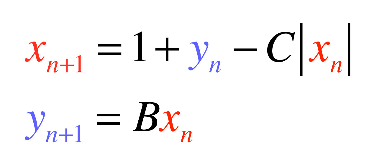
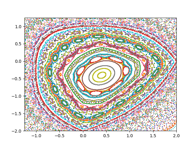
My favorite area-preserving discrete map is the Lozi Map. I first stumbled on this map at the very back of Steven Strogatz’ wonderful book on nonlinear dynamics [3]. It’s one of the last exercises of the last chapter. The map is particularly simple, but it leads to rich dynamics, both regular and chaotic. The map equations are
which is area-preserving when |B| = 1. The constant C can be varied, but the choice C = 0.5 works nicely, and B = -1 produces a beautiful nested structure, as shown in the figure.
Iterated Lozi map for B = -1 and C = 0.5. Each color is a distinct trajectory. Many regular trajectories exist that corral regions of chaotic trajectories. Trajectories become more chaotic farther away from the center.
Python Code for the Lozi Map
"""
Lozi.py
Created on Wed May  2 16:17:27 2018
@author: nolte
"""
import numpy as np
from scipy import integrate
from matplotlib import pyplot as plt

B = -1
C = 0.5

np.random.seed(2)
plt.figure(1)

for eloop in range(0,100):

    xlast = np.random.normal(0,1,1)
    ylast = np.random.normal(0,1,1)

    xnew = np.zeros(shape=(500,))
    ynew = np.zeros(shape=(500,))
    for loop in range(0,500):
        xnew[loop] = 1 + ylast - C*abs(xlast)
        ynew[loop] = B*xlast
        xlast = xnew[loop]
        ylast = ynew[loop]

    plt.plot(np.real(xnew),np.real(ynew),'o',ms=1)
    plt.xlim(xmin=-1.25,xmax=2)
    plt.ylim(ymin=-2,ymax=1.25)

plt.savefig('Lozi')
References:
[1] D. D. Nolte, “The Tangled Tale of Phase Space”, Chapter 6 in Galileo Unbound: A Path Across Life, the Universe and Everything (Oxford University Press, 2018)
[2] H. S. Dumas, The KAM Story: A Friendly Introduction to the Content, History, and Significance of Classical Kolmogorov-Arnold-Moser Theory (World Scientific, 2014)
[3] S. H. Strogatz, Nonlinear Dynamics and Chaos (WestView Press, 1994)