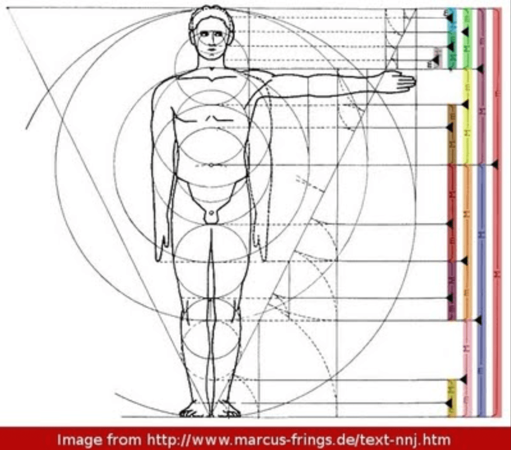
If ever there was a magic number that encoded the mysteries of the universe, then surely it must be the golden mean. It seems to pop up everywhere. In flowers and hurricanes. In pine cones and sea shells. In architecture and infinite sums. In telescoping cascades of golden rectangles in the human figure.
It also rears its head in the world of chaos theory, governing how a twisting dumbbell rotor transitions from regular motion to chaotic motion when it is tapped gently at a regular period.
The Golden Ratio
The Golden ratio can be defined in many ways, but its most common expression is given by
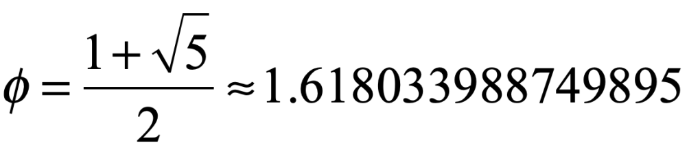
Among its many marvelous properties, one is that it is the hardest number to approximate with a ratio of small integers. For instance, the ratio 89/55 is a number that is as close as one part in ten thousand to the golden mean but it is hardly a ratio of small integers. This result may seem obscure, but there is a systematic way to find the ratios of integers that approximate an irrational number. This is known as continued fractions.
The continued fraction for the golden mean has an especially simple repeating form
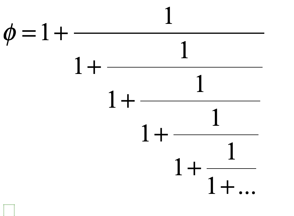
also written as
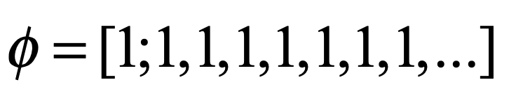
This continued fraction has the slowest convergence for its continued fraction of any other number. Hence, the Golden Ratio can be considered, using this criterion, to be the most irrational number of all, and it governs the last straw of order as chaos emerges from a surprisingly simple map.
The Kicked Rigid Rotor
The rigid rotator (the simple dumbbell) is one of the iconic systems in physics. It is a classic object in the study of rotational dynamics, showing up in Lagrangian formulations as well as Euler’s equations. It is also a classic system in elementary quantum mechanics, illustrating the quantization of angular momentum. In the current setting (Hamiltonian chaos), it is an example of a periodically perturbed system that displays beautiful phenomena.
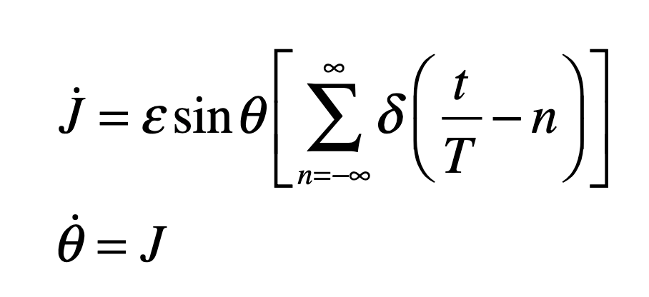
In chaos theory, the relationship between a continuous dynamical system and its discrete map is sometimes difficult to identify. However, a discrete map arises naturally from a randomly kicked dumbbell rotator. The system has an angular momentum J and a physical angle θ. The strength of the angular momentum kick is given by the perturbation parameter ε, and the torque of the kick is a function of the physical angle θ. The kicked rotator has the Hamiltonian
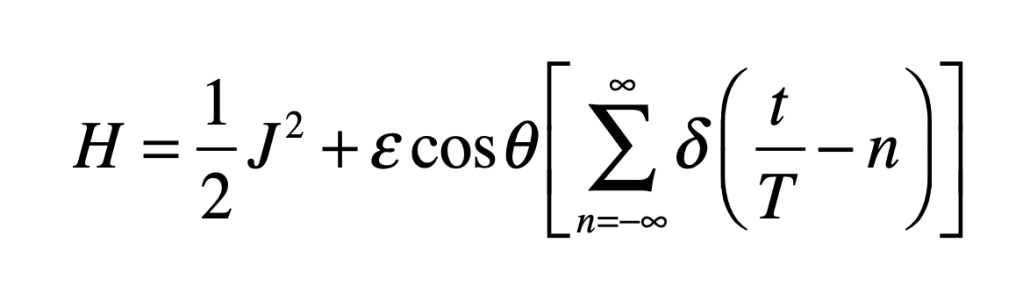
where the kicks are evenly timed with period T. The perturbation parameter ε can be large. The perturbation amplitude and sign depend on the instantaneous angle θ. The equations of motion from Hamilton’s equations are
The values for J and θ just before the nth successive kick are Jn and qn, respectively. Because the evaluation of the variables occurs at the period T, these discrete observations represent the values of a Poincaré section.
The Chirikov Twist Map
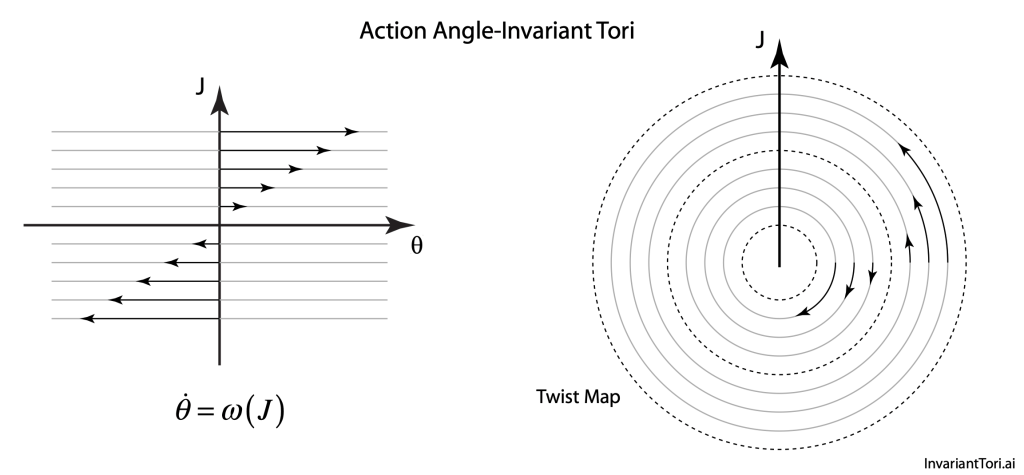
The phase space (in action-angle coordinates) of the rigid rotator is particularly attractive for applications because it is simply a linear flow that has increasing velocities with increasing action J. In action-angle representation, it is a twist map, where circles outside the radius for J = 0 twist in one direction but inside that radius they twist in the opposite direction. David Birkhoff showed in 1913, while proving Poincaré’s last geometric theorem, that a simple periodic perturbation of this system creates a set of closed trajectories (around an elliptical point) and a set of open trajectories (around a hyperbolic point).
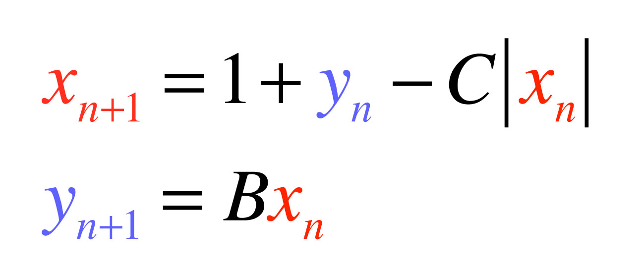
The rotator dynamics are continuous between each kick, leading to the discrete map (known as the Standard Map or the Chirikov Map)
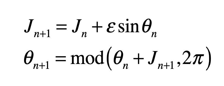
in which the rotator is “strobed”, or observed, at regular periods of 2π. When ε = 0, the orbits on the (θ, J) plane are simply horizontal lines—the rotator spins with regular motion at a speed determined by J.
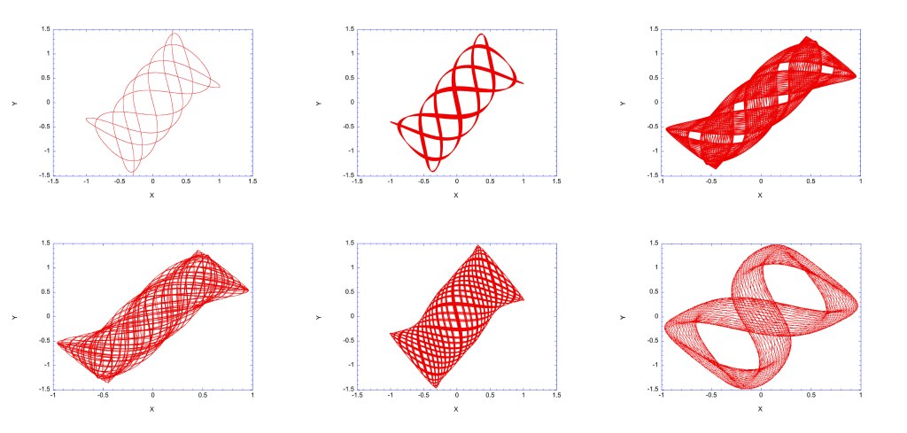
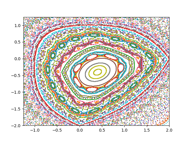
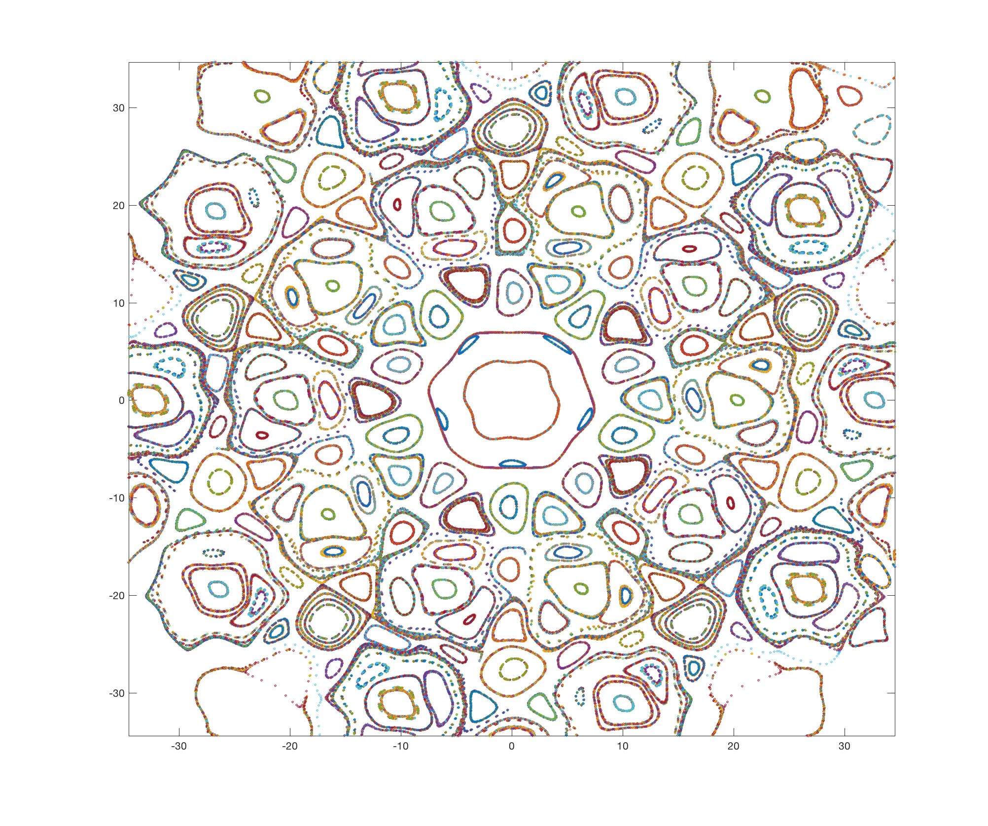
As the strength of the kick ε increases from zero, the Poicaré-Birkhoff theorem kicks in, and a first “island chain” appears with a single elliptical point paired with a single hyperbolic point. Then at larger values of ε new island chains appear, first with two islands, then with three, as in the figure below with ε = 0.3. Orbits that produce two islands are in a 2:1 resonance, and with three islands are in either a 3:1 or a 3:2 resonance. With increasing ε, more and more island chains open up, representing higher resonances.
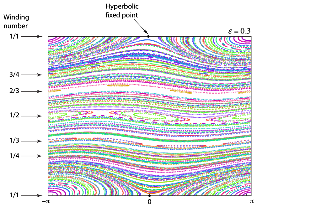
Each resonance is associated with a ratio of small integers: 1/2; 2/3; 3/4; 4/5 and beyond. These are the natural harmonics of the system. As the integers get larger, the ratios begin to approximate irrational numbers.
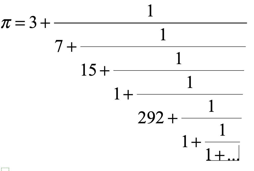
For instance, the number pi is approximated to increasing accuracy by the sequence of ratios:
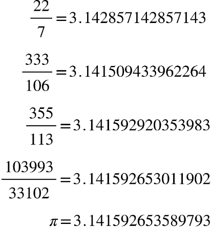
These are called convergents and are obtained by taking more terms in the continued fraction representation of pi.
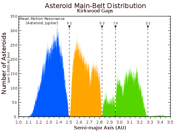
One of the fundamental findings of the theory of resonances in Hamiltonian systems is the decreasing “weight” of resonances associated with ratios of larger integers. Therefore, the 1:2 resonance is by far the most robust, the first to spring into existence, and it survives up to extremely strong perturbations. The 1:3 resonance is also relativety robust, but already the 1:4 and 1:5 resonances are more sensitive to perturbation and break up into island chains under moderate perturbation. Clearly the 22:7 ratio would not be sensitive nor the 333:106 resonance. These orbits would resist breaking up. Furthermore, once a resonance turns into an island chain, it creates hyperbolic points that can nucleate chaotic trajectories.
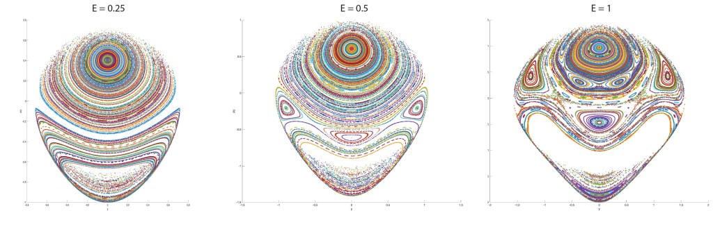
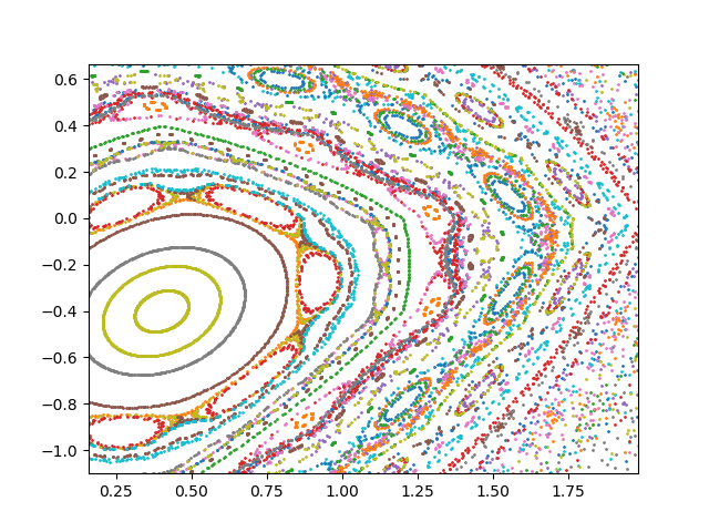
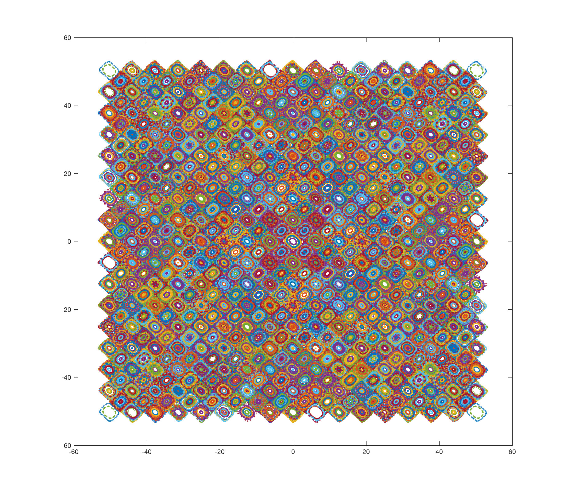
An example of the twist map at strong perturbation ε = 1.0 is shown in Fig. 4. There are numerous island chains. It is easy to find the 1:2 through the 1:7 resonances, but beyond that it is much more difficult to find these rational resonance. Furthermore, there are significant regions of chaotic trajectories associated with the hyperbolic points of the 1:2, 1:3, 1:4 and 1:5 resonances.
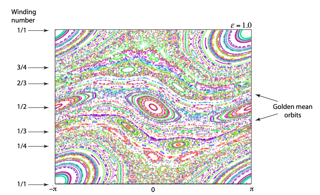
In the midst of the island chains and the chaos, there are still continuous (open) orbits that span the phase space without breaks. These are the most irrational numbers–numbers like the golden mean. These are the last orbits to break up. The critical threshold for the breakup of the golden-mean orbit is ε = 0.971. The plot in Fig. 4 is just above that threshold.
All of this behavior of the Standard Map follows from KAM theory, developed by Kolmogorov, Arnold and Moser in the early 1960’s. Although the standard map is specific to the tapped spinning disk, the results and behavior are very general for a wide class of two-dimensional Hamiltonian dynamical systems.
Adiabatic Following: Orbits of the Noble Means
The golden mean is not the only “slowest convergent” among irrational numbers. There are an entire class of irrational numbers whose continued fractions terminate with an infinite series of “1”s. These are known as the “Noble Means”. Examples are:
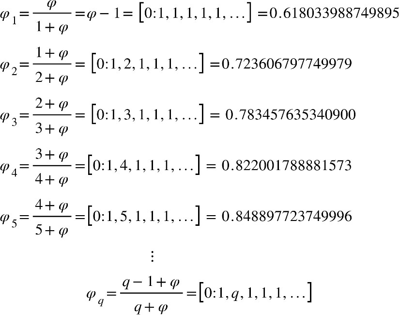
where the sequence, as q increases to infinity, converges on unity asymptotically among the set of irrationals with the slowest convergents.
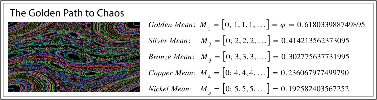
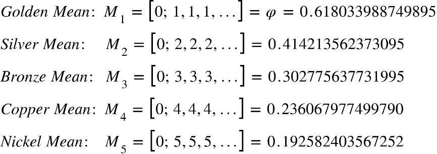
There are also the so-called “Metallic Means”, beginning with Gold and moving to Silver, Bronze, Copper, and Nickel. These are:
The challenge for numerical simulations is to find the orbits associated with these Metallic Means for large perturbation parameters ε. One cannot simply pick an initial condition for the Standard Map equal to a Metallic Mean, because at large perturbation, all the orbits have already shifted from their zero-perturbation values.
One of the most important principles in classical mechanics is the concept of adiabatic invariance. All the most common conservation laws of introductory physics–conservation of energy, momentum, and angular momentum–are consequences of adiabatic invariance. Indeed, the phase space of the rigid rotator is ideal for tracking adiabatic invariance because the J-value is the adiabatic invariant. In the numerical simulation, one begins with ε = 0, chooses an initial condition J = φn, and iterates the map as ε slowly increases.
This is shown in the following YouTube video. You will see five special orbits evolve as the perturbation is slowly increased. These are M1 (red), M2 (blue), M3 (green) and two resonances 3:1 (cyan) and 4:1 (magenta). The resonances are expected to break into island chains at relativity low perturbation ε, which is confirmed in the video.
Interestingly, the silver mean breaks into a 5:1 island chain around the same perturbation level. This is because the Silver Mean equals 0.414 which approaches 8/5 at moderate perturbation. Therefore, the Silver Mean orbit is “captured” by a 1:5 resonance and remains stable up to very large perturbations approaching ε = 1. The Bronze Mean is captured relativity early into the 1:1 resonance island.
References:
Music: The Beat Lessons (Band Camp): Link
D. D. Nolte, Introduction to Modern Dynamics, 2nd ed. (Oxford University Press, 2019) Link
This Post is Based on Simulations from Chapter 5 of IMD, 2nd edition
This Blog Post is a Companion to the undergraduate physics textbook Modern Dynamics: Chaos, Networks, Space and Time, 2nd ed. (Oxford, 2019) introducing Lagrangians and Hamiltonians, chaos theory, complex systems, synchronization, neural networks, econophysics and Special and General Relativity to Junior and Senior physics majors.