A chief principle of chaos theory states that even simple systems can display complex dynamics.  All that is needed for chaos, roughly, is for a system to have at least three dynamical variables plus some nonlinearity. 

A classic example of chaos is the driven damped pendulum.  This is a mass at the end of a massless rod driven by a sinusoidal perturbation.  The three variables are the angle, the angular velocity and the phase of the sinusoidal drive.  The nonlinearity is provided by the cosine function in the potential energy which is anharmonic for large angles.  However, the driven damped pendulum is not an autonomous system, because the drive is an external time-dependent function.  To find an autonomous system—one that persists in complex motion without any external driving function—one needs only to add one more mass to a simple pendulum to create what is known as a compound pendulum, or a double pendulum.

Daniel Bernoulli and the Discovery of Normal Modes

After the invention of the calculus by Newton and Leibniz, the first wave of calculus practitioners (Leibniz, Jakob and Johann Bernoulli and von Tschirnhaus) focused on static problems, like the functional form of the catenary (the shape of a hanging chain), or on constrained problems, like the brachistochrone (the path of least time for a mass under gravity to move between two points) and the tautochrone (the path of equal time).

The next generation of calculus practitioners (Euler, Johann and Daniel Bernoulli, and  D’Alembert) focused on finding the equations of motion of dynamical systems.  One of the simplest of these, that yielded the earliest equations of motion as well as the first identification of coupled modes, was the double pendulum.  The double pendulum, in its simplest form, is a mass on a rigid massless rod attached to another mass on a massless rod.  For small-angle motion, this is a simple coupled oscillator.

Daniel Bernoulli, the son of Johann I Bernoulli, was the first to study the double pendulum, publishing a paper on the topic in 1733 in the proceedings of the Academy in St. Petersburg just as he returned from Russia to take up a post permanently in his home town of Basel, Switzerland.  Because he was a physicist first and mathematician second, he performed experiments with masses on strings to attempt to understand the qualitative as well as quantitative behavior of the two-mass system.  He discovered that for small motions there was a symmetric behavior that had a low frequency of oscillation and an antisymmetric motion that had a higher frequency of oscillation.  Furthermore, he recognized that any general motion of the double pendulum was a combination of the fundamental symmetric and antisymmetric motions.  This work by Daniel Bernoulli represents the discovery of normal modes of coupled oscillators.  It is also the first statement of the combination of motions that he would use later (1753) to express for the first time the principle of superposition. 

Superposition is one of the guiding principles of linear physical systems.  It provides a means for the solution of differential equations.  It explains the existence of eigenmodes and their eigenfrequencies.  It is the basis of all interference phenomenon, whether classical like the Young’s double-slit experiment or quantum like Schrödinger’s cat.  Today, superposition has taken center stage in quantum information sciences and helps define the spooky (and useful) properties of quantum entanglement.  Therefore, normal modes, composition of motion, superposition of harmonics on a musical string—these all date back to Daniel Bernoulli in the twenty years between 1733 and 1753.  (Daniel Bernoulli is also the originator of the Bernoulli principle that explains why birds and airplanes fly.)

Johann Bernoulli and the Equations of Motion

Daniel Bernoulli’s father was Johann I Bernoulli.  Daniel had been tutored by Johann, along with his friend Leonhard Euler, when Daniel was young.  But as Daniel matured as a mathematician, he and his father began to compete against each other in international mathematics competitions (which were very common in the early eighteenth century).  When Daniel beat his father in a competition sponsored by the French Academy, Johann threw Daniel out of his house and their relationship remained strained for the remainder of their lives.

Johann had a history of taking ideas from Daniel and never citing the source. For instance, when Johann published his work on equations of motion for masses on strings in 1742, he built on the work of his son Daniel from 1733 but never once mentioned it. Daniel, of course, was not happy.

In a letter dated 20 October 1742 that Daniel wrote to Euler, he said, “The collected works of my father are being printed, and I have Just learned that he has inserted, without any mention of me, the dynamical problems I first discovered and solved (such as e. g. the descent of a sphere on a moving triangle; the linked pendulum, the center of spontaneous rotation, etc.).” And on 4 September 1743, when Daniel had finally seen his father’s works in print, he said, “The new mechanical problems are mostly mine, and my father saw my solutions before he solved the problems in his way …”. [2]

Daniel clearly has the priority for the discovery of the normal modes of the linked (i.e. double or compound) pendulum, but Johann often would “improve” on Daniel’s work despite giving no credit for the initial work. As a mathematician, Johann had a more rigorous approach and could delve a little deeper into the math. For this reason, it was Johann in 1742 who came closest to writing down differential equations of motion for multi-mass systems, but falling just short. It was D’Alembert only one year later who first wrote down the differential equations of motion for systems of masses and extended it to the loaded string for which he was the first to derive the wave equation. The D’Alembertian operator is today named after him.

Double Pendulum Dynamics

The general dynamics of the double pendulum are best obtained from Lagrange’s equations of motion. However, setting up the Lagrangian takes careful thought, because the kinetic energy of the second mass depends on its absolute speed which is dependent on the motion of the first mass from which it is suspended. The velocity of the second mass is obtained through vector addition of velocities.

The potential energy of the system is

so that the Lagrangian is

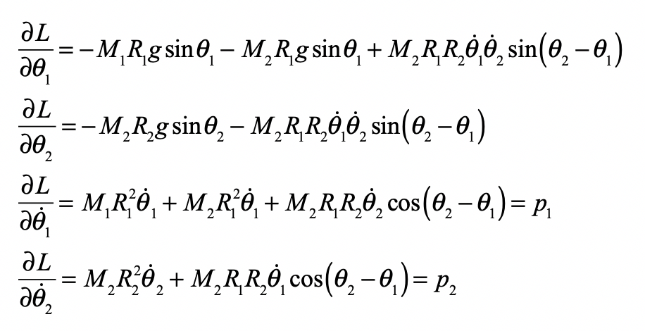
The partial derivatives are

and the time derivatives of the last two expressions are

Therefore, the equations of motion are

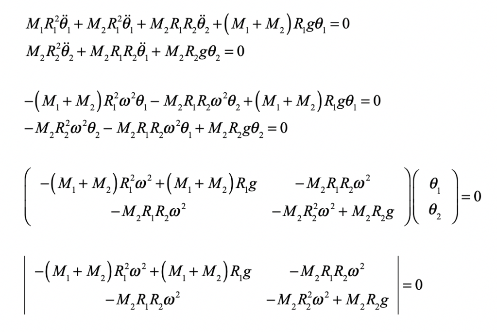
To get a sense of how this system behaves, we can make a small-angle approximation to linearize the equations to find the lowest-order normal modes.  In the small-angle approximation, the equations of motion become

where the determinant is

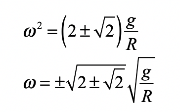
This quartic equation is quadratic in w2 and the quadratic solution is

This solution is still a little opaque, so taking the special case: R = R₁ = R₂ and M = M₁ = M₂ it becomes

There are two normal modes.  The low-frequency mode is symmetric as both masses swing (mostly) together, while the higher frequency mode is antisymmetric with the two masses oscillating against each other.  These are the motions that Daniel Bernoulli discovered in 1733.

It is interesting to note that if the string were rigid, so that the two angles were the same, then the lowest frequency would be 3/5 which is within 2% of the above answer but is certainly not equal.  This tells us that there is a slightly different angular deflection for the second mass relative to the first.

Chaos in the Double Pendulum

The full expression for the nonlinear coupled dynamics is expressed in terms of four variables (q₁, q₂, w₁, w₂).  The dynamical equations are

These can be put into the normal form for a four-dimensional flow as

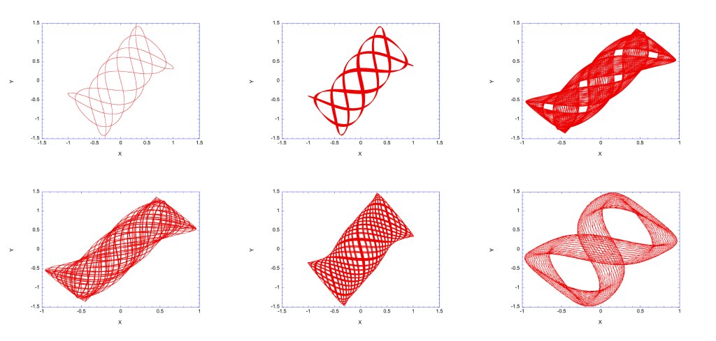
The numerical solution of these equations produce a complex interplay between the angle of the first mass and the angle of the second mass. Examples of trajectory projections in configuration space are shown in Fig. 3 for E = 1. The horizontal is the first angle, and the vertical is the angle of the second mass.

The dynamics in state space are four dimensional which are difficult to visualize directly. Using the technique of the Poincaré first-return map, the four-dimensional trajectories can be viewed as a two-dimensional plot where the trajectories pierce the Poincaré plane. Poincare sections are shown in Fig. 4.

Python Code: DoublePendulum.py

(Python code on GitHub.)

#!/usr/bin/env python3
# -*- coding: utf-8 -*-
"""
DoublePendulum.py
Created on Oct 16 06:03:32 2020
"Introduction to Modern Dynamics" 2nd Edition (Oxford, 2019)
@author: nolte
"""

import numpy as np
from scipy import integrate
from matplotlib import pyplot as plt
import time

plt.close('all')

E = 1.       # Try 0.8 to 1.5

def flow_deriv(x_y_z_w,tspan):
    x, y, z, w = x_y_z_w

    A = w**2*np.sin(y-x);
    B = -2*np.sin(x);
    C = z**2*np.sin(y-x)*np.cos(y-x);
    D = np.sin(y)*np.cos(y-x);
    EE = 2 - (np.cos(y-x))**2;
    
    FF = w**2*np.sin(y-x)*np.cos(y-x);
    G = -2*np.sin(x)*np.cos(y-x);
    H = 2*z**2*np.sin(y-x);
    I = 2*np.sin(y);
    JJ = (np.cos(y-x))**2 - 2;

    a = z
    b = w
    c = (A+B+C+D)/EE
    d = (FF+G+H+I)/JJ
    return[a,b,c,d]

repnum = 75

np.random.seed(1)
for reploop  in range(repnum):
    
    
    px1 = 2*(np.random.random((1))-0.499)*np.sqrt(E);
    py1 = -px1 + np.sqrt(2*E - px1**2);            

    xp1 = 0   # Try 0.1
    yp1 = 0   # Try -0.2
    
    x_y_z_w0 = [xp1, yp1, px1, py1]
    
    tspan = np.linspace(1,1000,10000)
    x_t = integrate.odeint(flow_deriv, x_y_z_w0, tspan)
    siztmp = np.shape(x_t)
    siz = siztmp[0]

    if reploop % 50 == 0:
        plt.figure(2)
        lines = plt.plot(x_t[:,0],x_t[:,1])
        plt.setp(lines, linewidth=0.5)
        plt.show()
        time.sleep(0.1)
        #os.system("pause")

    y1 = np.mod(x_t[:,0]+np.pi,2*np.pi) - np.pi
    y2 = np.mod(x_t[:,1]+np.pi,2*np.pi) - np.pi
    y3 = np.mod(x_t[:,2]+np.pi,2*np.pi) - np.pi
    y4 = np.mod(x_t[:,3]+np.pi,2*np.pi) - np.pi
    
    py = np.zeros(shape=(10*repnum,))
    yvar = np.zeros(shape=(10*repnum,))
    cnt = -1
    last = y1[1]
    for loop in range(2,siz):
        if (last < 0)and(y1[loop] > 0):
            cnt = cnt+1
            del1 = -y1[loop-1]/(y1[loop] - y1[loop-1])
            py[cnt] = y4[loop-1] + del1*(y4[loop]-y4[loop-1])
            yvar[cnt] = y2[loop-1] + del1*(y2[loop]-y2[loop-1])
            last = y1[loop]
        else:
            last = y1[loop]
     
    plt.figure(3)
    lines = plt.plot(yvar,py,'o',ms=1)
    plt.show()
    
plt.savefig('DPen')

You can change the energy E on line 16 and also the initial conditions xp1 and yp1 on lines 48 and 49. The energy E is the initial kinetic energy imparted to the two masses. For a given initial condition, what happens to the periodic orbits as the energy E increases?

References

[1] Daniel Bernoulli, Theoremata de oscillationibus corporum filo flexili connexorum et catenae verticaliter suspensae,” Academiae Scientiarum Imperialis Petropolitanae, 6, 1732/1733

[2] Truesdell B. The rational mechanics of flexible or elastic bodies, 1638-1788. (Turici: O. Fussli, 1960). (This rare and artistically produced volume, that is almost impossible to find today in any library, is one of the greatest books written about the early history of dynamics.)

This Blog Post is a Companion to the undergraduate physics textbook Modern Dynamics: Chaos, Networks, Space and Time, 2nd ed. (Oxford, 2019) introducing Lagrangians and Hamiltonians, chaos theory, complex systems, synchronization, neural networks, econophysics and Special and General Relativity.