Imagine in your mind the stately grandfather clock.  The long slow pendulum swinging back and forth so purposefully with such majesty.  It harks back to slower simpler times—seemingly Victorian in character, although their origins go back to Christiaan Huygens in 1656.  In introductory physics classes the dynamics of the pendulum is taught as one of the simplest simple harmonic oscillators, only a bit more complicated than a mass on a spring.

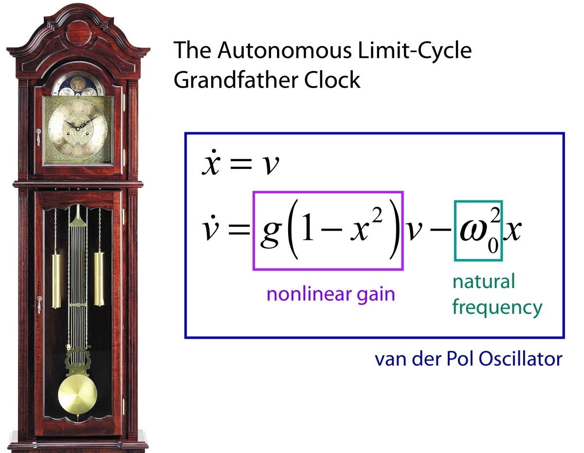
But don’t be fooled!  This simplicity is an allusion, for the pendulum clock lies at the heart of modern dynamics.  It is a nonlinear autonomous oscillator with system gain that balances dissipation to maintain a dynamic equilibrium that ticks on resolutely as long as some energy source can continue to supply it (like the heavy clock weights).    

This analysis has converted the two-dimensional dynamics of the autonomous oscillator to a simple one-dimensional dynamics with a stable fixed point.

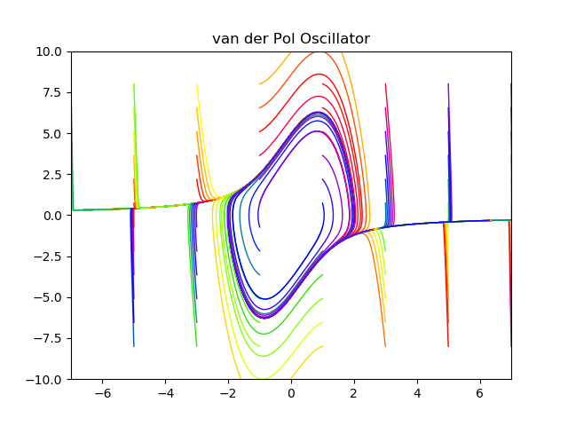
The dynamic equilibrium of the grandfather clock is known as a limit cycle, and they are the central feature of autonomous oscillators.  Autonomous oscillators are one of the building blocks of complex systems, providing the fundamental elements for biological oscillators, neural networks, business cycles, population dynamics, viral epidemics, and even the rings of Saturn.  The most famous autonomous oscillator (after the pendulum clock) is named for a Dutch physicist, Balthasar van der Pol (1889 – 1959), who discovered the laws that govern how electrons oscillate in vacuum tubes.  But this highly specialized physics problem has expanded to become the new guiding paradigm for the fundamental oscillating element of modern dynamics—the van der Pol oscillator.

The van der Pol Oscillator

The van der Pol (vdP) oscillator begins as a simple harmonic oscillator (SHO) in which the dissipation (loss of energy) is flipped to become gain of energy.  This is as simple as flipping the sign of the damping term in the SHO

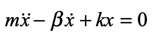
where β is positive.  This 2^nd-order ODE is re-written into a dynamical flow as

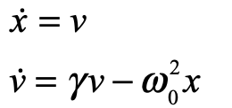
where γ = β/m is the system gain.  Clearly, the dynamics of this SHO with gain would lead to run-away as the oscillator grows without bound.             

But no real-world system can grow indefinitely.  It has to eventually be limited by things such as inelasticity.  One of the simplest ways to include such a limiting process in the mathematical model is to make the gain get smaller at larger amplitudes.  This can be accomplished by making the gain a function of the amplitude x as

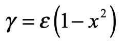
When the amplitude x gets large, the gain decreases, becoming zero and changing sign when x = 1.  Putting this amplitude-dependent gain into the SHO equation yields

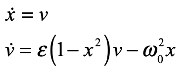
This is the van der Pol equation.  It is the quintessential example of a nonlinear autonomous oscillator.            

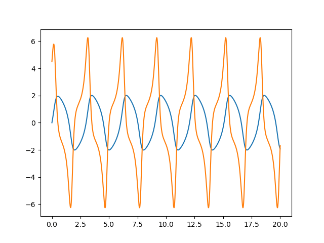
When the parameter ε is large, the vdP oscillator has can behave in strongly nonlinear ways, with strongly nonlinear and nonharmonic oscillations.  An example is shown in Fig. 2 for a = 5 and b = 2.5.  The oscillation is clearly non-harmonic.

#!/usr/bin/env python3
# -*- coding: utf-8 -*-
"""
Created on Mon Apr 16 07:38:57 2018
@author: David Nolte
D. D. Nolte, Introduction to Modern Dynamics: Chaos, Networks, Space and Time, 2nd ed. (Oxford,2019)
"""
import numpy as np
from scipy import integrate
from matplotlib import pyplot as plt

plt.close('all')

def solve_flow(param,lim = [-3,3,-3,3],max_time=10.0):
# van der pol 2D flow 
    def flow_deriv(x_y, t0, alpha,beta):
        x, y = x_y
        return [y,-alpha*x+beta*(1-x**2)*y]
    
    plt.figure()
    xmin = lim[0]
    xmax = lim[1]
    ymin = lim[2]
    ymax = lim[3]
    plt.axis([xmin, xmax, ymin, ymax])

    N=144
    colors = plt.cm.prism(np.linspace(0, 1, N))
    
    x0 = np.zeros(shape=(N,2))
    ind = -1
    for i in range(0,12):
        for j in range(0,12):
            ind = ind + 1;
            x0[ind,0] = ymin-1 + (ymax-ymin+2)*i/11
            x0[ind,1] = xmin-1 + (xmax-xmin+2)*j/11
             
    # Solve for the trajectories
    t = np.linspace(0, max_time, int(250*max_time))
    x_t = np.asarray([integrate.odeint(flow_deriv, x0i, t, param)
                      for x0i in x0])

    for i in range(N):
        x, y = x_t[i,:,:].T
        lines = plt.plot(x, y, '-', c=colors[i])
        plt.setp(lines, linewidth=1)

    plt.show()
    plt.title(model_title)
    plt.savefig('Flow2D')
    
    return t, x_t

def solve_flow2(param,max_time=20.0):
# van der pol 2D flow 
    def flow_deriv(x_y, t0, alpha,beta):
        #"""Compute the time-derivative of a Medio system."""
        x, y = x_y
        return [y,-alpha*x+beta*(1-x**2)*y]
    model_title = 'van der Pol Oscillator'
    x0 = np.zeros(shape=(2,))
    x0[0] = 0
    x0[1] = 4.5
    
    # Solve for the trajectories
    t = np.linspace(0, max_time, int(250*max_time))
    x_t = integrate.odeint(flow_deriv, x0, t, param)
 
    return t, x_t

param = (5, 2.5)             # van der Pol
lim = (-7,7,-10,10)

t, x_t = solve_flow(param,lim)

t, x_t = solve_flow2(param)
plt.figure(2)
lines = plt.plot(t,x_t[:,0],t,x_t[:,1],'-')

Separation of Time Scales

Nonlinear systems can have very complicated behavior that may be difficult to address analytically.  This is why the numerical ODE solver is a central tool of modern dynamics.  But there is a very neat analytical trick that can be applied to tame the nonlinearities (if they are not too large) and simplify the autonomous oscillator.  This trick is called separation of time scales (also known as secular perturbation theory)—it looks for simultaneous fast and slow behavior within the dynamics.  An example of fast and slow time scales in a well-known dynamical system is found in the simple spinning top in which nutation (fast oscillations) are superposed on precession (slow oscillations).             

For the autonomous van der Pol oscillator the fast time scale is the natural oscillation frequency, while the slow time scale is the approach to the limit cycle.  Let’s assign t₀ = t and t₁ = εt, where ε is a small parameter.  t₀ is the slow period (approach to the limit cycle) and t₁ is the fast period (natural oscillation frequency).  The solution in terms of these time scales is

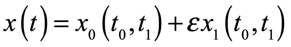
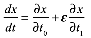
where x₀ is a slow response and acts as an envelope function for x₁ that is the fast response. The total differential is

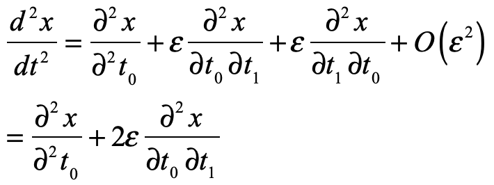
Similarly, to obtain a second derivative

Therefore, the vdP equation in terms of x₀ and x₁ is

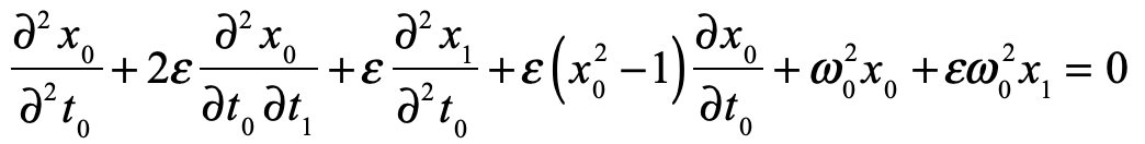
to lowest order. Now separate the orders to zeroth and first orders in ε, respectively,

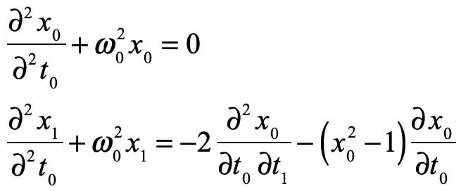
Solve the first equation (a simple harmonic oscillator)

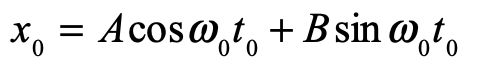
and plug the solution it into the right-hand side of the second equation to give

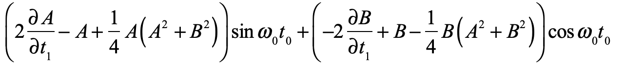
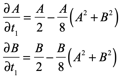
The key to secular perturbation theory is to confine dynamics to their own time scales.  In other words, the slow dynamics provide the envelope that modulates the fast carrier frequency.  The envelope dynamics are contained in the time dependence of the coefficients A and B.  Furthermore, the dynamics of x₁ should be a homogeneous function of time, which requires each term in the last equation to be zero.  Therefore, the dynamical equations for the envelope functions are

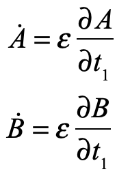
These can be transformed into polar coordinates. Because the envelope functions do not depend on the slow time scale, the time derivatives are

With these expressions, the slow dynamics become

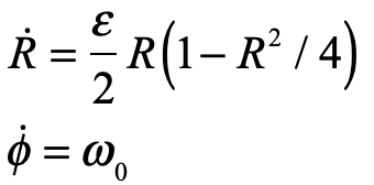
where the angular velocity in the fast variable is equal to zero, leaving only the angular velocity of the unperturbed oscillator. (This is analogous to the rotating wave approximation (RWA) in optics, and also equivalent to studying the dynamics in the rotating frame of the unperturbed oscillator.)

Making a final substitution ρ = R/2 gives a very simple set of dynamical equations

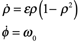
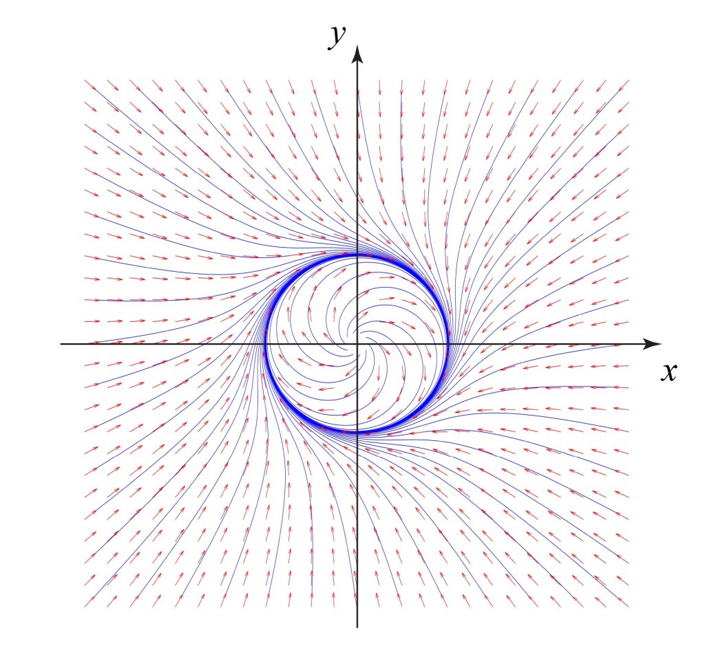
These final equations capture the essential properties of the relaxation of the dynamics to the limit cycle. To lowest order (when the gain is weak) the angular frequency is unaffected, and the system oscillates at the natural frequency. The amplitude of the limit cycle equals 1. A deviation in the amplitude from 1 decays slowly back to the limit cycle making it a stable fixed point in the radial dynamics. This analysis has converted the two-dimensional dynamics of the autonomous oscillator to a simple one-dimensional dynamics with a stable fixed point on the radius variable. The phase-space portrait of this simplified autonomous oscillator is shown in Fig. 3. What could be simpler? This simplified autonomous oscillator can be found as a fundamental element of many complex systems.

Further Reading

D. D. Nolte, Introduction to Modern Dynamics: Chaos, Networks, Space and Time, 2nd edition (Oxford University Press, 2019)

Pikovsky, A. S., M. G. Rosenblum and J. Kurths (2003). Synchronization: A Universal concept in nonlinear science. Cambridge, Cambridge University Press.

This Blog Post is a Companion to the undergraduate physics textbook Modern Dynamics: Chaos, Networks, Space and Time, 2nd ed. (Oxford, 2019) introducing Lagrangians and Hamiltonians, chaos theory, complex systems, synchronization, neural networks, econophysics and Special and General Relativity.