There is no greater geometric solid than the simplex. It is the paragon of efficiency, the pinnacle of symmetry, and the prototype of simplicity. If the universe were not constructed of continuous coordinates, then surely it would be tiled by tessellations of simplices.
Indeed, simplices, or simplexes, arise in a wide range of geometrical problems and real-world applications. For instance, metallic alloys are described on a simplex to identify the constituent elements [1]. Zero-sum games in game theory and ecosystems in population dynamics are described on simplexes [2], and the Dantzig simplex algorithm is a central algorithm for optimization in linear programming [3]. Simplexes also are used in nonlinear minimization (amoeba algorithm), in classification problems in machine learning, and they also raise their heads in quantum gravity. These applications reflect the special status of the simplex in the geometry of high dimensions.
… It’s Simplexes all the way down!
The reason for their usefulness is the simplicity of their construction that guarantees a primitive set that is always convex. For instance, in any space of d-dimensions, the simplest geometric figure that can be constructed of flat faces to enclose a d-volume consists of d+1 points that is the d-simplex.
Or …
In any space of d-dimensions, the simplex is the geometric figure whose faces are simplexes, whose faces are simplexes, whose faces are again simplexes, and those faces are once more simplexes … And so on.
In other words, it’s simplexes all the way down.
Simplex Geometry
In this blog, I will restrict the geometry to the regular simplex. The regular simplex is the queen of simplexes: it is the equilateral simplex for which all vertices are equivalent, and all faces are congruent, and all sub-faces are congruent, and so on. The regular simplexes have the highest symmetry properties of any polytope. A polytope is the d-dimensional generalization of a polyhedron. For instance, the regular 2-simplex is the equilateral triangle, and the regular 3-simplex is the equilateral tetrahedron.
The N-simplex is the high-dimensional generalization of the tetrahedron. It is a regular N-dimensional polytope with N+1 vertexes. Starting at the bottom and going up, the simplexes are the point (0-simplex), the unit line (1-simplex), the equilateral triangle (2-simplex), the tetrahedron (3-simplex), the pentachoron (4-simplex), the hexateron (5-simplex) and onward. When drawn on the two-dimensional plane, the simplexes are complete graphs with links connecting every node to every other node. This dual character of equidistance and completeness give simplexes their utility. Each node is equivalent and is linked to each other. There are N•(N-1)/2 links among N vertices, and there are (N-2)•(N-1)/2 triangular faces.
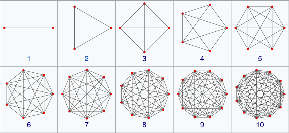
Construction of a d-simplex is recursive: Begin with a (d-1)-dimensional simplex and add a point along an orthogonal dimension to construct a d-simplex. For instance, to create a 2-simplex (an equilateral triangle), find the mid-point of the 1-simplex (a line segment)
Centered 1-simplex: (-1), (1)
add a point on the perpendicular that is the same distance from each original vertex as the original vertices were distant from each other
Off-centered 2-simplex: (-1,0), (1,0), (0, sqrt(3)/2)
Then shift the origin to the center of mass of the triangle
Centered 2-simplex: (-1, -sqrt(3)/6), (1, -sqrt(3)/6), (0, sqrt(3)/3)
The 2-simplex, i.e., the equilateral triangle, has a 1-simplex as each of its faces. And each of those 1-simplexes has a 0-simplex as each of its ends. Therefore, this recursive construction of ever higher-dimensional simplexes out of low-dimensional ones, provides an interesting pattern:
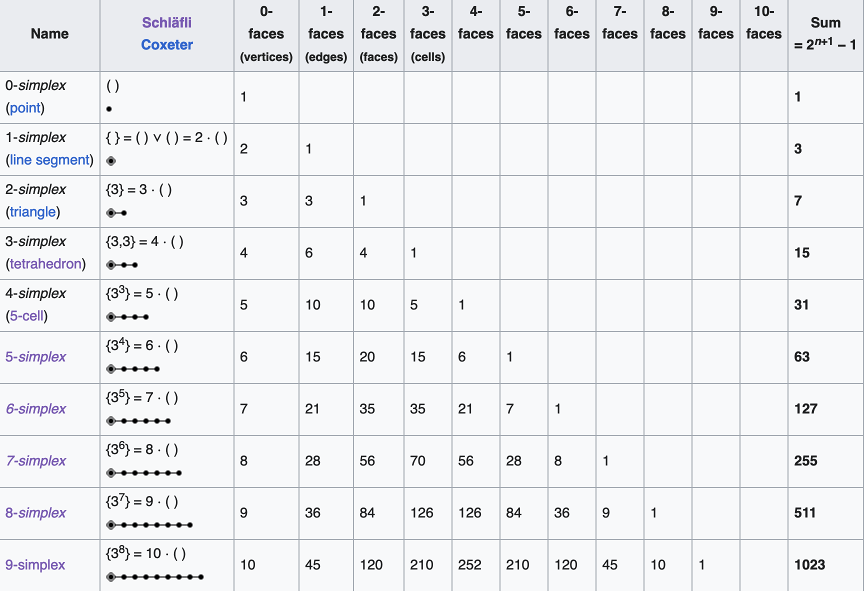
The coordinates of an N-simplex are not unique, although there are several convenient conventions. One convention defines standard coordinates for an N-simplex in N+1 coordinate bases. These coordinates embed the simplex into a space of one higher dimension. For instance, the standard 2-simplex is defined by the coordinates (001), (010), (100) forming a two-dimensional triangle in three dimensions, and the simplex is a submanifold in the embedding space. A more efficient coordinate choice matches the coordinate-space dimensionality to the dimensionality of the simplex. Hence the 10 vertices of a 9-simplex can be defined by 9 coordinates (also not unique). One choice is given in Fig. 4 for the 1-simplex up to the 9-simplex.

The equations for the simplex coordinates are
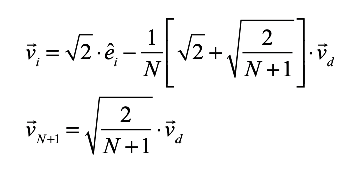
where

is the “diagonal” vector. These coordinates are centered on the center of mass of the simplex, and the links all have length equal to 2 which can be rescaled by a multiplying factor. The internal dihedral angle between all of the coordinate vectors for an N-simplex is

For moderate to high-dimensionality, the position vectors of the simplex vertices are pseudo-orthogonal. For instance, for N = 9 the dihedral angle cosine is -1/9 = -0.111. For higher dimensions, the simplex position vectors become asymptotically orthogonal. Such orthogonality is an important feature for orthonormal decomposition of class superpositions, for instance of overlapping images.
Alloy Mixtures and Barycentric Coordinates
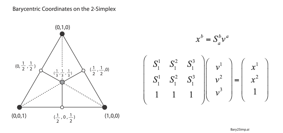
For linear systems, the orthonormality of basis representations is one of the most powerful features for system analysis in terms of superposition of normal modes. Neural networks, on the other hand, are intrinsically nonlinear decision systems for which linear superposition does not hold inside the network, even if the symbols presented to the network are orthonormal superpositions. This loss of orthonormality in deep networks can be partially retrieved by selecting the Simplex code. It has pseudo-orthogonal probability distribution functions located on the vertices of the simplex. There is an additional advantage to using the Simplex code: by using so-called barycentric coordinates, the simplex vertices can be expressed as independent bases. An example for the 2-simplex is shown in Fig. 5. The x-y Cartesian coordinates of the vertices (using tensor index notation) are given by (S11, S12), (S21, S22), and (S31, S32). Any point (x1, x2) on the plane can be expressed as a linear combination of the three vertices with barycentric coordinates (v1, v2, v3) by solving for these three coefficients from the equation
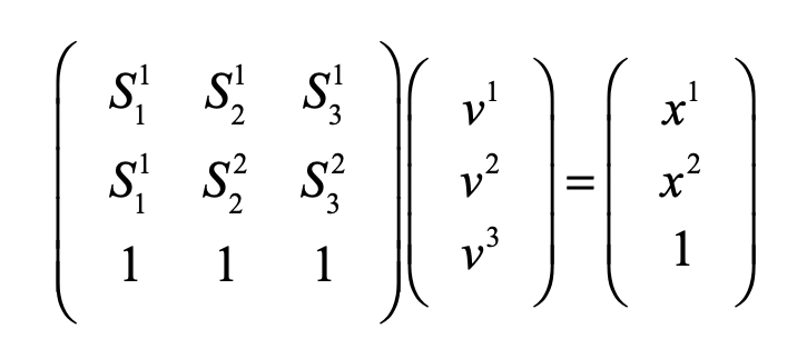
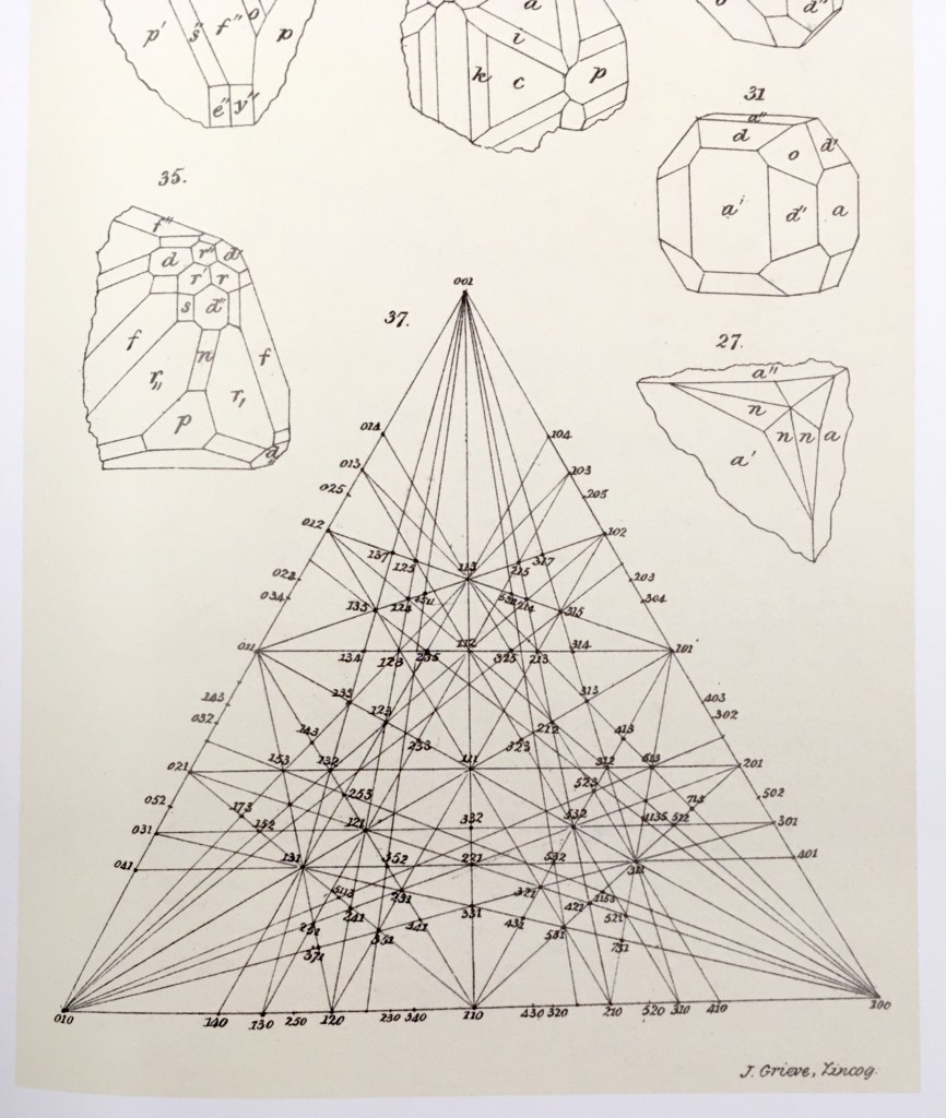
using Cramers rule. For instance, the three vertices of the simplex are expressed using the 3-component barycentric coordinates (1,0,0), (0,1,0) and (0,0,1). The mid-points on the edges have barycentric coordinates (1/2,1/2,0), (0,1/2,1/2), and (1/2,0,1/2). The centroid of the simplex has barycentric coordinates (1/3,1/3,1/3). Barycentric coordinates on a simplex are commonly used in phase diagrams of alloy systems in materials science. The simplex can also be used to identify crystallographic directions in three-dimensions, as in Fig. 6.
Replicator Dynamics on the Simplex
Ecosystems are among the most complex systems on Earth. The complex interactions among hundreds or thousands of species may lead to steady homeostasis in some cases, to growth and collapse in other cases, and to oscillations or chaos in yet others. But the definition of species can be broad and abstract, referring to businesses and markets in economic ecosystems, or to cliches and acquaintances in social ecosystems, among many other examples. These systems are governed by the laws of evolutionary dynamics that include fitness and survival as well as adaptation. The dimensionality of the dynamical spaces for these systems extends to hundreds or thousands of dimensions—far too complex to visualize when thinking in four dimensions is already challenging.
A classic model of interacting species is the replicator equation. It allows for a fitness-based proliferation and for trade-offs among the individual species. The replicator dynamics equations are shown in Fig. 7.

The population dynamics on the 2D simplex are shown in Fig. 8 for several different pay-off matrices (square matrix to the upper left of each simplex). The matrix values are shown in color and help interpret the trajectories. For instance the simplex on the upper-right shows a fixed point center. This reflects the antisymmetric character of the pay-off matrix around the diagonal. The stable spiral on the lower-left has a nearly asymmetric pay-off matrix, but with unequal off-diagonal magnitudes. The other two cases show central saddle points with stable fixed points on the boundary. A large variety of behaviors are possible for this very simple system. The Python program can be found in Trirep.py.

Linear Programming with the Dantzig Simplex
There is a large set of optimization problems in which a linear objective function is to be minimized subject to a set of inequalities. This is known as “Linear Programming”. These LP systems can be expressed as

The vector index goes from 1 to d, the dimension of the space. Each inequality creates a hyperplane, where two such hyperplanes intersect along a line terminated at each end by a vertex point. The set of vertexes defines a polytope in d-dimensions, and each face of the polytope, when combined with the point at the origin, defines a 3-simplex.
It is easy to visualize in lower dimensions why the linear objective function must have an absolute minimum at one of the vertexes of the polytope. And finding that minimum is a trivial exercise: Start at any vertex. Poll each neighboring vertex and move to the one that has the lowest value of the objective function. Repeat until the current vertex has a lower objective value than any neighbors. Because of the linearity of the objective function, this is a unique minimum (except for rare cases of accidental degeneracy). This iterative algorithm defines a walk on the vertexes of the polytope.
The question arises, why not just evaluate the objection function at each vertex and then just pick the vertex with the lowest value? The answer in high dimensions is that there are too many vertexes, and finding all of them is inefficient. If there are N vertexes, the walk to the solution visits only a few of the vertexes, on the order of log(N). The algorithm therefore scales as log(N), just like a search tree.

This simple algorithm was devised by George Dantzig (1914 – 2005) in 1939 when he was a graduate student at UC Berkeley. He had arrived late to class and saw two problems written on the chalk board. He assumed that these were homework assignments, so he wrote them down and worked on them over the following week. He recalled that they seemed a bit harder than usual, but he eventually solved them and turned them in. A few weeks later, his very excited professor approached him and told him that the problems weren’t homework–they were two of the most important outstanding problems in optimization and that Dantzig had just solved them! The 1997 movie Good Will Hunting, with Matt Damon, Ben Affleck, and Robin Williams, borrowed this story for the opening scene.
The Amoeba Simplex Crawling through Hyperspace
Unlike linear programming problems with linear objective functions, multidimensional minimization of nonlinear objective functions is an art unto itself, with many approach. One of these is a visually compelling algorithm that does the trick more often than not. This is the so-called amoeba algorithm that shares much in common with the Dantzig simplex approach to linear programming, but instead of a set of fixed simplex coordinates, it uses a constantly shifting d-dimensional simplex that “crawls” over the objective function, seeking its minimum.
One of the best descriptions of the amoeba simplex algorithm is in “Numerical Recipes” [4] that describes the crawling simplex as
When it reaches a “valley floor”, the method contracts itself in the transverse direction and tries to ooze down the valley. If there is a situation where the simplex is trying to “pass through the eye of a needle”, it contracts itself in all directions, pulling itself in around its lowest (best) point.
(From Press, Numerical Recipes, Cambridge)
The basic operations for the crawling simplex are reflection and scaling. For a given evaluation of all the vertexes of the simplex, one will have the highest value and another the lowest. In a reflection, the highest point is reflected through the d-dimensional face defined by the other d vertexes. After reflection, if the new evaluation is lower than the former lowest value, then the point is expanded. If, on the other hand, it is little better than it was before reflection, then the point is contracted. The expansion and contraction are what allows the algorithm to slide through valleys or shrink to pass through the eye of a needle.
The amoeba algorithm was developed by John Nelder and Roger Mead in 1965 at a time when computing power was very limited. The algorithm works great as a first pass at a minimization problem, and it almost always works for moderately small dimensions, but for very high dimensions there are more powerful algorithms today for optimization, built into all the deep learning software environments like Tensor Flow and the Matlab toolbox.
By David D. Nolte, May 3, 2023
[1] M. Hillert, Phase equilibria, phase diagrams and phase transformations : their thermodynamic basis. (Cambridge University Press, Cambridge, UK ;, ed. 2nd ed., 2008).
[2] P. Schuster, K. Sigmund, Replicator Dynamics. Journal of Theoretical Biology 100, 533-538 (1983); P. Godfrey-Smith, The replicator in retrospect. Biology & Philosophy 15, 403-423 (2000).
[3] R. E. Stone, C. A. Tovey, The Simplex and Projective Scaling Algorithms as Iteratively Reweighted Least-squares Methods. Siam Review 33, 220-237 (1991).
[4] W. H. Press, Numerical Recipes in C++ : The Art of Scientific Computing. (Cambridge University Press, Cambridge, UK; 2nd ed., 2002).


