
Heisenberg’s uncertainty principle is a law of physics – it cannot be violated under any circumstances, no matter how much we may want it to yield or how hard we try to bend it. Heisenberg, as he developed his ideas after his lone epiphany like a monk on the isolated island of Helgoland off the north coast of Germany in 1925, became a bit of a zealot, like a religious convert, convinced that all we can say about reality is a measurement outcome. In his view, there was no independent existence of an electron other than what emerged from a measuring apparatus. Reality, to Heisenberg, was just a list of numbers in a spread sheet—matrix elements. He took this line of reasoning so far that he stated without exception that there could be no such thing as a trajectory in a quantum system. When the great battle commenced between Heisenberg’s matrix mechanics against Schrödinger’s wave mechanics, Heisenberg was relentless, denying any reality to Schrödinger’s wavefunction other than as a calculation tool. He was so strident that even Bohr, who was on Heisenberg’s side in the argument, advised Heisenberg to relent [1]. Eventually a compromise was struck, as Heisenberg’s uncertainty principle allowed Schrödinger’s wave functions to exist within limits—his uncertainty limits.
Disaster in the Poconos
Yet the idea of an actual trajectory of a quantum particle remained a type of heresy within the close quantum circles. Years later in 1948, when a young Richard Feynman took the stage at a conference in the Poconos, he almost sabotaged his career in front of Bohr and Dirac—two of the giants who had invented quantum mechanics—by having the audacity to talk about particle trajectories in spacetime diagrams.
Feynman was making his first presentation of a new approach to quantum mechanics that he had developed based on path integrals. The challenge was that his method relied on space-time graphs in which “unphysical” things were allowed to occur. In fact, unphysical things were required to occur, as part of the sum over many histories of his path integrals. For instance, a key element in the approach was allowing electrons to travel backwards in time as positrons, or a process in which the electron and positron annihilate into a single photon, and then the photon decays back into an electron-positron pair—a process that is not allowed by mass and energy conservation. But this is a possible history that must be added to Feynman’s sum.
It all looked like nonsense to the audience, and the talk quickly derailed. Dirac pestered him with questions that he tried to deflect, but Dirac persisted like a raven. A question was raised about the Pauli exclusion principle, about whether an orbital could have three electrons instead of the required two, and Feynman said that it could—all histories were possible and had to be summed over—an answer that dismayed the audience. Finally, as Feynman was drawing another of his space-time graphs showing electrons as lines, Bohr rose to his feet and asked derisively whether Feynman had forgotten Heisenberg’s uncertainty principle that made it impossible to even talk about an electron trajectory.
It was hopeless. The audience gave up and so did Feynman as the talk just fizzled out. It was a disaster. What had been meant to be Feynman’s crowning achievement and his entry to the highest levels of theoretical physics, had been a terrible embarrassment. He slunk home to Cornell where he sank into one of his depressions. At the close of the Pocono conference, Oppenheimer, the reigning king of physics, former head of the successful Manhattan Project and newly selected to head the prestigious Institute for Advanced Study at Princeton, had been thoroughly disappointed by Feynman.
But what Bohr and Dirac and Oppenheimer had failed to understand was that as long as the duration of unphysical processes was shorter than the energy differences involved, then it was literally obeying Heisenberg’s uncertainty principle. Furthermore, Feynman’s trajectories—what became his famous “Feynman Diagrams”—were meant to be merely cartoons—a shorthand way to keep track of lots of different contributions to a scattering process. The quantum processes certainly took place in space and time, conceptually like a trajectory, but only so far as time durations, and energy differences and locations and momentum changes were all within the bounds of the uncertainty principle. Feynman had invented a bold new tool for quantum field theory, able to supply deep results quickly. But no one at the Poconos could see it.

Coherent States
When Feynman had failed so miserably at the Pocono conference, he had taken the stage after Julian Schwinger, who had dazzled everyone with his perfectly scripted presentation of quantum field theory—the competing theory to Feynman’s. Schwinger emerged the clear winner of the contest. At that time, Roy Glauber (1925 – 2018) was a young physicist just taking his PhD from Schwinger at Harvard, and he later received a post-doc position at Princeton’s Institute for Advanced Study where he became part of a miniature revolution in quantum field theory that revolved around—not Schwinger’s difficult mathematics—but Feynman’s diagrammatic method. So Feynman won in the end. Glauber then went on to Caltech, where he filled in for Feynman’s lectures when Feynman was off in Brazil playing the bongos. Glauber eventually returned to Harvard where he was already thinking about the quantum aspects of photons in 1956 when news of the photon correlations in the Hanbury-Brown Twiss (HBT) experiment were published. Three years later, when the laser was invented, he began developing a theory of photon correlations in laser light that he suspected would be fundamentally different than in natural chaotic light.
Because of his background in quantum field theory, and especially quantum electrodynamics, it was fairly easy to couch the quantum optical properties of coherent light in terms of Dirac’s creation and annihilation operators of the electromagnetic field. Glauber developed a “coherent state” operator that was a minimum uncertainty state of the quantized electromagnetic field, related to the minimum-uncertainty wave functions derived initially by Schrödinger in the late 1920’s. The coherent state represents a laser operating well above the lasing threshold and behaved as “the most classical” wavepacket that can be constructed. Glauber was awarded the Nobel Prize in Physics in 2005 for his work on such “Glauber states” in quantum optics.
Quantum Trajectories
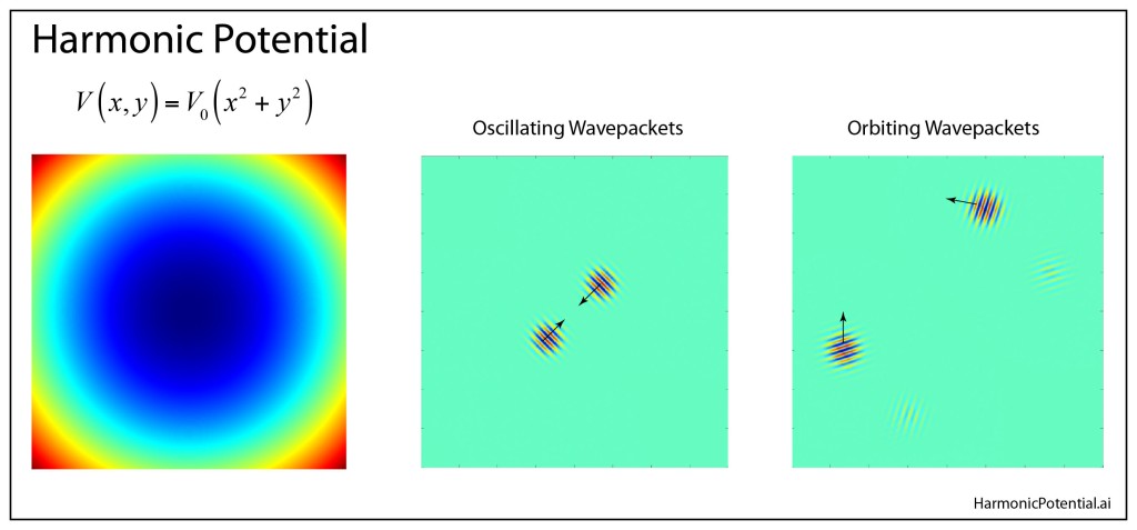
Glauber’s coherent states are built up from the natural modes of a harmonic oscillator. Therefore, it should come as no surprise that these coherent-state wavefunctions in a harmonic potential behave just like classical particles with well-defined trajectories. The quadratic potential matches the quadratic argument of the the Gaussian wavepacket, and the pulses propagate within the potential without broadening, as in Fig. 3, showing a snapshot of two wavepackets propagating in a two-dimensional harmonic potential. This is a somewhat radical situation, because most wavepackets in most potentials (or even in free space) broaden as they propagate. The quadratic potential is a special case that is generally not representative of how quantum systems behave.
To illustrate this special status for the quadratic potential, the wavepackets can be launched in a potential with a quartic perturbation. The quartic potential is anharmonic—the frequency of oscillation depends on the amplitude of oscillation unlike for the harmonic oscillator, where amplitude and frequency are independent. The quartic potential is integrable, like the harmonic oscillator, and there is no avenue for chaos in the classical analog. Nonetheless, wavepackets broaden as they propagate in the quartic potential, eventually spread out into a ring in the configuration space, as in Fig. 4.
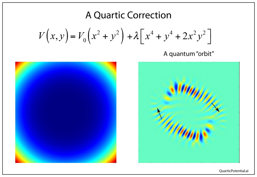
A potential with integrability has as many conserved quantities to the motion as there are degrees of freedom. Because the quartic potential is integrable, the quantum wavefunction may spread, but it remains highly regular, as in the “ring” that eventually forms over time. However, integrable potentials are the exception rather than the rule. Most potentials lead to nonintegrable motion that opens the door to chaos.
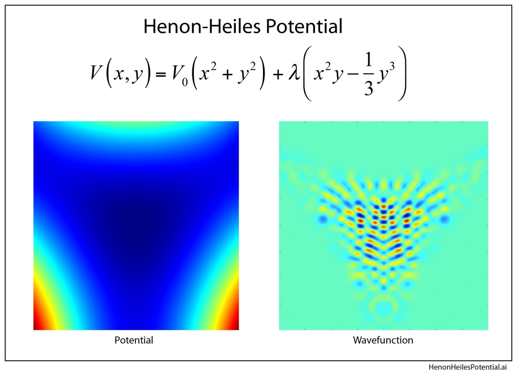
A classic (and classical) potential that exhibits chaos in a two-dimensional configuration space is the famous Henon-Heiles potential. This has a four-dimensional phase space which admits classical chaos. The potential has a three-fold symmetry which is one reason it is non-integral, since a particle must “decide” which way to go when it approaches a saddle point. In the quantum regime, wavepackets face the same decision, leading to a breakup of the wavepacket on top of a general broadening. This allows the wavefunction eventually to distribute across the entire configuration space, as in Fig. 5.
Youtube Video
Movies of quantum trajectories can be viewed at my Youtube Channel, Physics Unbound. The answer to the question “Is there a quantum trajectory?” can be seen visually as the movies run—they do exist in a very clear sense under special conditions, especially coherent states in a harmonic oscillator. And the concept of a quantum trajectory also carries over from a classical trajectory in cases when the classical motion is integrable, even in cases when the wavefunction spreads over time. However, for classical systems that display chaotic motion, wavefunctions that begin as coherent states break up into chaotic wavefunctions that fill the accessible configuration space for a given energy. The character of quantum evolution of coherent states—the most classical of quantum wavefunctions—in these cases reflects the underlying character of chaotic motion in the classical analogs. This process can be seen directly watching the movies as a wavepacket approaches a saddle point in the potential and is split. Successive splits of the multiple wavepackets as they interact with the saddle points is what eventually distributes the full wavefunction into its chaotic form.
Therefore, the idea of a “quantum trajectory”, so thoroughly dismissed by Heisenberg, remains a phenomenological guide that can help give insight into the behavior of quantum systems—both integrable and chaotic.
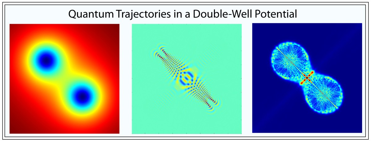
As a side note, the laws of quantum physics obey time-reversal symmetry just as the classical equations do. In the third movie of “A Quantum Ballet“, wavefunctions in a double-well potential are tracked in time as they start from coherent states that break up into chaotic wavefunctions. It is like watching entropy in action as an ordered state devolves into a disordered state. But at the half-way point of the movie, the imaginary part of the wavefunction has its sign flipped, and the dynamics continue. But now the wavefunctions move from disorder into an ordered state, seemingly going against the second law of thermodynamics. Flipping the sign of the imaginary part of the wavefunction at just one instant in time plays the role of a time-reversal operation, and there is no violation of the second law.
By David D. Nolte, Sept. 4, 2022
YouTube Video
YouTube Video of Quantum Trajectories
For more on the history of quantum trajectories, see Galileo Unbound from Oxford Press:

References
[1] See Chapter 8 , On the Quantum Footpath, in Galileo Unbound, D. D. Nolte (Oxford University Press, 2018)
[2] J. R. Nagel, A Review and Application of the Finite-Difference Time-Domain Algorithm Applied to the Schrödinger Equation, ACES Journal, Vol. 24, NO. 1, pp. 1-8 (2009)

[…] Is There a Quantum Trajectory? […]
LikeLike