Ada Lovelace at the Dawn of Cyber Steampunk

Something strange almost happened in 1840’s England just a few years into Queen Victoria’s long reign—a giant machine the size of a large shed, built of thousands of interlocking steel gears, driven by steam power, almost came to life—a thinking, mechanical automaton, the very image of Cyber Steampunk.

Cyber Steampunk is a genre of media that imagines an alternate history of a Victorian Age with advanced technology—airships and rockets and robots and especially computers—driven by steam power.  Some of the classics that helped launch the genre are the animé movies Castle in the Sky (1986) by Hayao Miyazaki and Steam Boy (2004) by Katsuhiro Otomo and the novel The Difference Engine (1990) by William Gibson and Bruce Sterling.  The novel pursues Ada Byron, Lady Lovelace, through the shadows of London by those who suspect she has devised a programmable machine that can win at gambling using steam and punched cards.  This is not too far off from what might have happened in real life if Ada Lovelace had a bit more sway over one of her unsuitable suitors—Charles Babbage. 

But Babbage, part genius, part fool, could not understand what Lovelace understood—for if he had, a Victorian computer built of oiled gears and leaky steam pipes, instead of tiny transistors and metallic leads, might have come a hundred years early as another marvel of the already marvelous Industrial Revolution.  How might our world today be different if Babbage had seen what Lovelace saw?

Fig. 1 Sony Entertainment Ad for Steamboy (2004).

Boundless Babbage

There is no question of Babbage’s genius.  He was so far ahead of his time that he appeared to most people in his day to be a crackpot, and he was often treated as one.  His father thought he was useless, and he told him so, because to be a scientist in the early 1800’s was to be unemployable, and Babbage was unemployed for years after college.  Science was, literally, natural philosophy, and no one hired a philosopher unless they were faculty at some college.  But Babbage’s friends from Trinity College, Cambridge, like William Whewell (future dean of Trinity) and John Herschel (son of the famous astronomer), new his worth and were loyal throughout their lives and throughout his trials.

Fig. 2 Charles Babbage

Charles Babbage was a favorite at Georgian dinner parties because he was so entertaining to watch and to listen to.  From personal letters of his friends (and enemies) of the time one gets a picture of a character not too different from Sheldon Cooper on the TV series The Big Bang Theory—convinced of his own genius and equally convinced of the lack of genius of everyone else and ready to tell them so.  His mind was so analytic, that he talked like a walking computer—although nothing like a computer existed in those days—everything was logic and functions and propositions—hence his entertainment value.  No one understood him, and no one cared—until he ran into a young woman who actually did, but more of that later.

One summer day in 1821, Babbage and Herschel were working on mathematical tables for the Astrophysical Society, a dull but important job to ensure that star charts and moon positions could be used accurately for astronomical calculations and navigation.  The numbers filled column after column, page after page. But as they checked the values, the two were shocked by how many entries in the tables were wrong.  In that day, every numerical value of every table or chart was calculated by a person (literally called a computer), and people make mistakes.  Even as they went to correct the numbers, new mistakes would crop in.  In frustration, Babbage exclaimed to Herschel that what they needed was a steam-powered machine that would calculate the numbers automatically.  No sooner had he said it, than Babbage had a vision of a mechanical machine, driven by a small steam engine, full of gears and rods, that would print out the tables automatically without flaws.

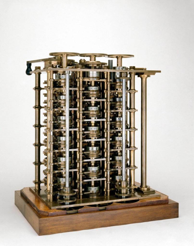
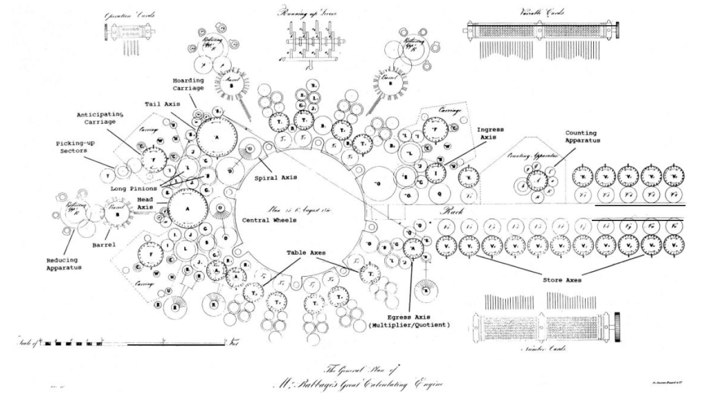
Being unemployed (and unemployable) Babbage had enough time on his hands to actually start work on his engine.  He called it the Difference Engine because it worked on the Method of Differences—mathematical formulas were put into a form where a number was expressed as a series, and the differences between each number in the series would be calculated by the engine.  He approached the British government for funding, and it obliged with considerable funds.  In the days before grant proposals and government funding, Babbage had managed to jump start his project and, in a sense, gain employment.  His father was not impressed, but he did not live long enough to see what his son Charles could build.  Charles inherited a large sum from his father (the equivalent of about 14 million dollars today), which further freed him to work on his Difference Engine.  By 1832, he had finally completed a seventh part of the Engine and displayed it in his house for friends and visitors to see. 

This working section of the Difference Engine can be seen today in the London Science Museum.  It is a marvel of steel and brass, consisting of three columns of stacked gears whose enmeshed teeth represent digital numbers.  As a crank handle is turned, the teath work upon each other, generating new numbers through the permutations of rotated gear teeth.  Carrying tens was initially a problem for Babbage, as it is for school children today, but he designed an ingenious mechanical system to accomplish the carry.

Fig. 3 One-seventh part of Babbage’s Difference Engine.

All was going well, and the government was pleased with progress, until Charles had a better idea that threatened to scrap all he had achieved.  It is not known how this new idea came into being, but it is known that it happened shortly after he met the amazing young woman: Ada Byron.

Lovely Lovelace

Ada Lovelace, born Ada Byron, had the awkward distinction of being the only legitimate child of Lord Byron, lyric genius and poet.  Such was Lord Byron’s hedonist lifestyle that no-one can say for sure how many siblings Ada had, not even Lord Byron himself, which was even more awkward when his half-sister bore a bastard child that may have been his.

Fig. 4 Ada Lovelace

Ada’s high-born mother prudently divorced the wayward poet and was not about to have Ada pulled into her father’s morass.  Where Lord Byron was bewitched (some would say possessed) by art and spirit, the mother sought an antidote, and she encouraged Ada to study hard cold mathematics.  She could not have known that Ada too had a genius like her father’s, only aimed differently, bewitched by the beauty in the sublime symbols of math. 

An insight into the precocious child’s way of thinking can be gained from a letter that the 12-year-old girl wrote to her mother who was off looking for miracle cures for imaginary ills. At that time in 1828, in a confluence of historical timelines in the history of mathematics, Ada and her mother (and Ada’s cat Puff) were living at Bifrons House which was the former estate of Brook Taylor, who had developed the Taylor’s series a hundred years earlier in 1715. In Ada’s letter, she describes a dream she had of a flying machine, which is not so remarkable, but then she outlined her plan to her mother to actually make one, which is remarkable. As you read her letter, you see she is already thinking about weights and material strengths and energy efficiencies, thinking like an engineer and designer—at the age of only 12 years!

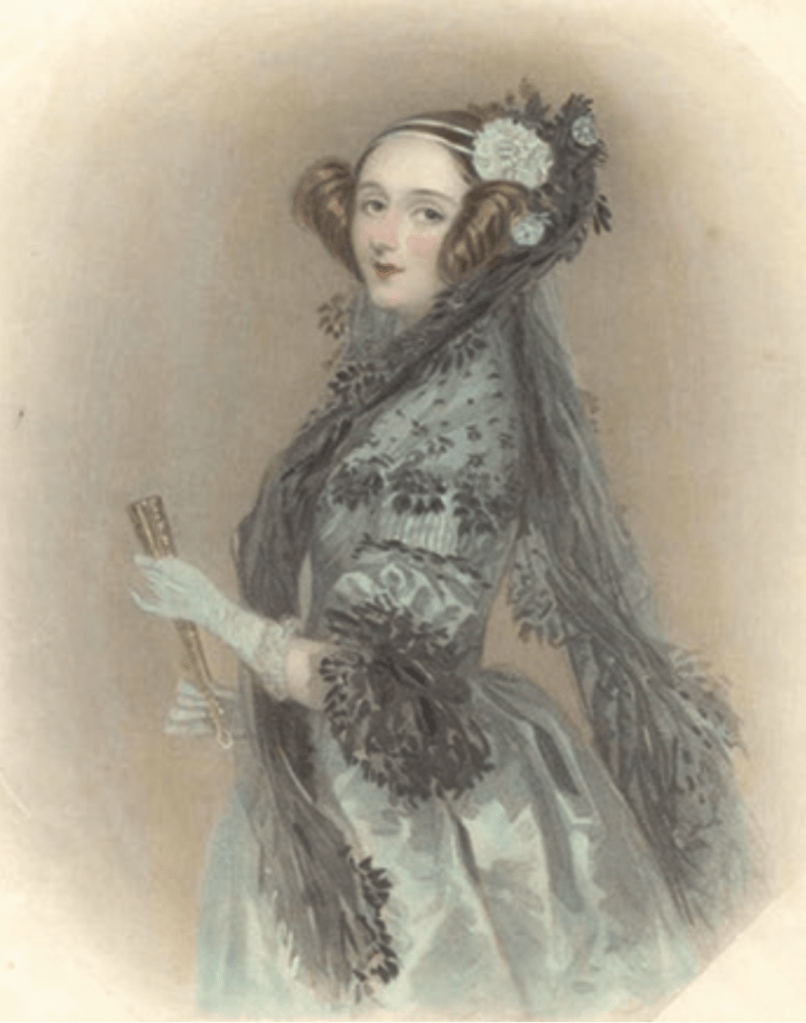
In later years, Lovelace would become the Enchantress of Number to a number of her mathematical friends, one of whom was the strange man she met at a dinner party in the summer of 1833 when she was 17 years old.  The strange man was Charles Babbage, and when he talked to her about his Difference Engine, expecting to be tolerated as an entertaining side show, she asked pertinent questions, one after another, and the two became locked in conversation. 

Babbage was a recent widower, having lost his wife with whom he had been happily compatible, and one can only imagine how he felt when the attractive and intelligent woman gave him her attention.  But Ada’s mother would never see Charles as a suitable husband for her daughter—she had ambitious plans for her, and she tolerated Babbage only as much as she did because of the affection that Ada had for him.  Nonetheless, Ada and Charles became very close as friends and met frequently and wrote long letters to each other, discussing problems and progress on the Difference Engine.

In December of 1834, Charles invited Lady Byron and Ada to his home where he described with great enthusiasm a vision he had of an even greater machine.  He called it his Analytical Engine, and it would surpass his Difference Engine in a crucial way:  where the Difference Engine needed to be reconfigured by hand before every new calculation, the Analytical Engine would never need to be touched, it just needed to be programmed with punched cards.  Charles was in top form as he wove his narrative, and even Lady Byron was caught up in his enthusiasm.  The effect on Ada, however, was nothing less than a religious conversion. 

Fig. 5 General block diagram of Babbage’s Analytical Engine. From [8].

Ada’s Notes

To meet Babbage as an equal, Lovelace began to study mathematics with an obsession, or one might say, with delusions of grandeur.  She wrote “I believe myself to possess a most singular combination of qualities exactly fitted to make me pre-eminently a discoverer of the hidden realities of nature,” and she was convinced that she was destined to do great things.

Then, in 1835, Ada was married off to a rich but dull aristocrat who was elevated by royal decree to the Earldom of Lovelace, making her the Countess of Lovelace.  The marriage had little effect on Charles’ and Ada’s relationship, and he was invited frequently to the new home where they continued their discussions about the Analytical Engine. 

By this time Charles had informed the British government that he was putting all his effort into the design his new machine—news that was not received favorably since he had never delivered even a working Difference Engine.  Just when he hoped to start work on his Analytical Engine, the government ministers pulled their money. This began a decade’s long ordeal for Babbage as he continued to try to get monetary support as well as professional recognition from his peers for his ideas. Neither attempt was successful at home in Britain, but he did receive interest abroad, especially from a future prime minister of Italy, Luigi Menabrae, who invited Babbage to give a lecture in Turin on his Analytical Engine. Menabrae later had the lecture notes published in French. When Charles Wheatstone, a friend of Babbage, learned of Menabrae’s publication, he suggested to Lovelace that she translate it into English. Menabrae’s publication was the only existing exposition of the Analytical Engine, because Babbage had never written on the Engine himself, and Wheatstone was well aware of Lovelace’s talents, expecting her to be one of the only people in England who had the ability and the connections to Babbage to accomplish the task.

Ada Lovelace dove into the translation of Menabrae’s “Sketch of the Analytical Engine Invented by Charles Babbage” with the single-mindedness that she was known for. Along with the translation, she expanded on the work with Notes of her own that she added, lettered from A to G. By the time she wrote them, Lovelace had become a top-rate mathematician, possibly surpassing even Babbage, and her Notes were three times longer than the translation itself, providing specific technical details and mathematical examples that Babbage and Menabrae only allude to.

On a different level, the character of Ada’s Notes stands in stark contrast to Charles’ exposition as captured by Menabrae: where Menabrae provided only technical details of Babbage’s Engine, Lovelace’s Notes captured the Engine’s potential. She was still a poet by disposition—that inheritance from her father was never lost.

Lovelace wrote:

We may say most aptly, that the Analytical Engine weaves algebraic patterns just as the Jacquard-loom weaves flowers and leaves.

Here she is referring to the punched cards that the Jacquard loom used to program the weaving of intricate patterns into cloth. Babbage had explicitly borrowed this function from Jacquard, adapting it to provide the programmed input to his Analytical Engine.

But it was not all poetics. She also saw the abstract capabilities of the Engine, writing

In studying the action of the Analytical Engine, we find that the peculiar and independent nature of the considerations which in all mathematical analysis belong to operations, as distinguished from the objects operated upon and from the results of the operations performed upon those objects, is very strikingly defined and separated.

Again, it might act upon other things besides number, where objects found whose mutual fundamental relations could be expressed by those of the abstract science of operations, and which should be also susceptible of adaptations to the action of the operating notation and mechanism of the engine.

Supposing, for instance, that the fundamental relations of pitched sounds in the science of harmony and of musical composition were susceptible of such expression and adaptations, the engine might compose elaborate and scientific pieces of music of any degree of complexity or extent.

Here she anticipates computers generating musical scores.

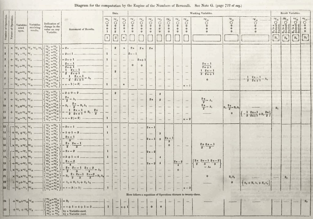
Most striking is Note G. This is where she explicitly describes how the Engine would be used to compute numerical values as solutions to complicated problems. She chose, as her own example, the calculation of Bernoulli numbers which require extensive numerical calculations that were exceptionally challenging even for the best human computers of the day. In Note G, Lovelace writes down the step-by-step process by which the Engine would be programmed by the Jacquard cards to carry out the calculations. In the history of computer science, this stands as the first computer program.

Fig. 6 Table from Lovelace’s Note G on her method to calculate Bernoulli numbers using the Analytical Engine.

When it was time to publish, Babbage read over Lovelace’s notes, checking for accuracy, but he appears to have been uninterested in her speculations, possibly simply glossing over them. He saw his engine as a calculating machine for practical applications. She saw it for what we know today to be the exceptional adaptability of computers to all realms of human study and activity. He did not see what she saw. He was consumed by his Engine to the same degree as she, but where she yearned for the extraordinary, he sought funding for the mundane costs of machining and materials.

Ada’s Business Plan Pitch

Ada Lovelace watched in exasperation as Babbage floundered about with ill-considered proposals to the government while making no real progress towards a working Analytical Engine. Because of her vision into the potential of the Engine, a vision that struck her to her core, and seeing a prime opportunity to satisfy her own yearning to make an indelible mark on the world, she despaired in ever seeing it brought to fruition. Charles, despite his genius, was too impractical, wasting too much time on dead ends and incapable of performing the deft political dances needed to attract support. She, on the other hand, saw the project clearly and had the time and money and the talent, both mathematically and through her social skills, to help.

On Monday August 14, 1843, Ada wrote what might be the most heart-felt and impassioned business proposition in the history of computing. She laid out in clear terms to Charles how she could advance the Analytical Engine to completion if only he would surrender to her the day-to-day authority to make it happen. She was, in essence, proposing to be the Chief Operating Officer in a disruptive business endeavor that would revolutionize thinking machines a hundred years before their time. She wrote (she liked to underline a lot):

Firstly: I want to know whether if I continue to work on & about your own great subject, you will undertake to abide wholly by the judgment of myself (or of any persons whom you may now please to name as referees, whenever we may differ), on all practical matters relating to whatever can involve relations with any fellow-creature or fellow-creatures.

Secondly: can you undertake to give your mind wholly & undividedly, as a primary object that no engagement is to interfere with, to the consideration of all those matters in which I shall at times require your intellectual assistance & supervision; & can you promise not to slur & hurry things over; or to mislay, & allow confusion and mistakes to enter into documents, &c?

Thirdly: if I am able to lay before you in the course of a year or two, explicit & honorable propositions for executing your engine, (such as are approved by persons whom you may now name to be referred to for their approbation), would there be any chance of your allowing myself & such parties to conduct the business for you; your own undivided energies being devoted to the execution of the work; & all other matters being arranged for you on terms which your own friends should approve?

This is a remarkable letter from a self-possessed 28-year-old woman, laying out in explicit terms how she proposed to take on the direction of the project, shielding Babbage from the problems of relating to other people or “fellow-creatures” (which was his particular weakness), giving him time to focus his undivided attention on the technical details (which was his particular strength), while she would be the outward face of the project that would attract the appropriate funding.

In her preface to her letter, Ada adroitly acknowledges that she had been a romantic disappointment to Charles, but she pleads with him not to let their personal history cloud his response to her proposal. She also points out that her keen intellect would be an asset to the project and asks that he not dismiss it because of her sex (which a biased Victorian male would likely do). Despite her entreaties, this is exactly what Babbage did. Pencilled on the top of the original version of Ada’s letter in the Babbage archives is his simple note: “Tuesday 15 saw AAL this morning and refused all the conditions”. He had not even given her proposal 24 hours consideration as he indeed slurred and hurried things over.

Aftermath

Babbage never constructed his Analytical Engine and never even wrote anything about it. All his efforts would have been lost to history if Alan Turing had not picked up on Ada’s Notes and expanded upon them a hundred years later, bringing both her and him to the attention of the nascent computing community.

Ada Lovelace died young in 1852, at the age of 36, of cancer. By then she had moved on from Babbage and was working on other things. But she never was able to realize her ambition of uncovering such secrets of nature as to change the world.

Ada had felt from an early age that she was destined for greatness. She never achieved it in her lifetime and one can only wonder what she thought about this as she faced her death. Did she achieve it in posterity? This is a hotly debated question. Some say she wrote the first computer program, which may be true, but little programming a hundred years later derived directly from her work. She did not affect the trajectory of computing history. Discovering her work after the fact is interesting, but cannot be given causal weight in the history of science. The Vikings were the first Europeans to discover America, but no-one knew about it. They did not affect subsequent history the way that Columbus did.

On the other hand, Ada has achieved greatness in a different way. Now that her story is known, she stands as an exemplar of what scientific and technical opportunities look like, and the risk of ignoring them. Babbage also did not achieve greatness during his lifetime, but he could have—if he had not dismissed her and her intellect. He went to his grave embittered rather than lauded because he passed up an opportunity he never recognized.

By David D. Nolte, June 26, 2023


References

[1] Facsimile of “Sketch of the Analytical Engine Invented by Charles Babbage” translated by Ada Lovelace from Harvard University.

[2] Facsimile of Ada Lovelace’s “Notes by the Translator“.

[3] Stephen Wolfram, “Untangling the Tale of Ada Lovelace“, Wolfram Writings (2015).

[4] J. Essinger, “Charles and Ada : The computer’s most passionate partnership,” (History Press, 2019).

[5] D. Swade, The Difference Engine: Charles Babbage and the quest to build the first computer (Penguin Books, 2002).

[6] W. Gibson, and B. Sterling, The Difference Engine (Bantam Books, 1992).

[7] L. J. Snyder, The Philosophical Breakfast Club : Four remarkable friends who transformed science and changed the world (Broadway Books, 2011).

[8] Allan G. Bromley, Charles Babbage’s Analytical Engine, 1838, Annals of the History of Computing, Volume 4, Number 3, July 1982, pp. 196 – 217

The Mighty Simplex

There is no greater geometric solid than the simplex.  It is the paragon of efficiency, the pinnacle of symmetry, and the prototype of simplicity.  If the universe were not constructed of continuous coordinates, then surely it would be tiled by tessellations of simplices.

Indeed, simplices, or simplexes, arise in a wide range of geometrical problems and real-world applications.  For instance, metallic alloys are described on a simplex to identify the constituent elements [1].  Zero-sum games in game theory and ecosystems in population dynamics are described on simplexes [2], and the Dantzig simplex algorithm is a central algorithm for optimization in linear programming [3].  Simplexes also are used in nonlinear minimization (amoeba algorithm), in classification problems in machine learning, and they also raise their heads in quantum gravity.  These applications reflect the special status of the simplex in the geometry of high dimensions.

… It’s Simplexes all the way down!

The reason for their usefulness is the simplicity of their construction that guarantees a primitive set that is always convex.  For instance, in any space of d-dimensions, the simplest geometric figure that can be constructed of flat faces to enclose a d-volume consists of d+1 points that is the d-simplex. 

Or …

In any space of d-dimensions, the simplex is the geometric figure whose faces are simplexes, whose faces are simplexes, whose faces are again simplexes, and those faces are once more simplexes … And so on. 

In other words, it’s simplexes all the way down.

Simplex Geometry

In this blog, I will restrict the geometry to the regular simplex.  The regular simplex is the queen of simplexes: it is the equilateral simplex for which all vertices are equivalent, and all faces are congruent, and all sub-faces are congruent, and so on.  The regular simplexes have the highest symmetry properties of any polytope. A polytope is the d-dimensional generalization of a polyhedron.  For instance, the regular 2-simplex is the equilateral triangle, and the regular 3-simplex is the equilateral tetrahedron.

The N-simplex is the high-dimensional generalization of the tetrahedron.  It is a regular N-dimensional polytope with N+1 vertexes.  Starting at the bottom and going up, the simplexes are the point (0-simplex), the unit line (1-simplex), the equilateral triangle (2-simplex), the tetrahedron (3-simplex), the pentachoron (4-simplex), the hexateron (5-simplex) and onward.  When drawn on the two-dimensional plane, the simplexes are complete graphs with links connecting every node to every other node.  This dual character of equidistance and completeness give simplexes their utility. Each node is equivalent and is linked to each other.  There are N•(N-1)/2 links among N vertices, and there are (N-2)•(N-1)/2 triangular faces.

Fig. 1  The N-simplex structures from 1-D through 10-D.  Drawn on the 2D plane, the simplexes are complete graphs with links between every node.  The number of vertices is equal to the number of dimensions plus one. (Wikipedia)
Fig. 2 Coulomb-spring visualization of the energy minimization of a 12-simplex (a 12-dimensional tetrahedron). Each node is a charge. Each link is a spring. Beginning as a complete graph on the planar circle, it finds a minimum configuration with 3 internal nodes.

Construction of a d-simplex is recursive:  Begin with a (d-1)-dimensional simplex and add a point along an orthogonal dimension to construct a d-simplex.  For instance, to create a 2-simplex (an equilateral triangle), find the mid-point of the 1-simplex (a line segment)

            Centered 1-simplex:                (-1), (1)    

add a point on the perpendicular that is the same distance from each original vertex as the original vertices were distant from each other     

            Off-centered 2-simplex:         (-1,0), (1,0), (0, sqrt(3)/2)

Then shift the origin to the center of mass of the triangle

            Centered 2-simplex:               (-1, -sqrt(3)/6), (1, -sqrt(3)/6), (0, sqrt(3)/3)

The 2-simplex, i.e., the equilateral triangle, has a 1-simplex as each of its faces.  And each of those 1-simplexes has a 0-simplex as each of its ends.  Therefore, this recursive construction of ever higher-dimensional simplexes out of low-dimensional ones, provides an interesting pattern:

Fig. 3 The entries are the same numbers that appear in Pascal’s Triangle. (Wikipedia)

The coordinates of an N-simplex are not unique, although there are several convenient conventions.  One convention defines standard coordinates for an N-simplex in N+1 coordinate bases.  These coordinates embed the simplex into a space of one higher dimension.  For instance, the standard 2-simplex is defined by the coordinates (001), (010), (100) forming a two-dimensional triangle in three dimensions, and the simplex is a submanifold in the embedding space.  A more efficient coordinate choice matches the coordinate-space dimensionality to the dimensionality of the simplex.  Hence the 10 vertices of a 9-simplex can be defined by 9 coordinates (also not unique).  One choice is given in Fig. 4 for the 1-simplex up to the 9-simplex. 

Fig. 4 One possible set of coordinates for the 1-simplex up to the 9-simplex.  The center of mass of the simplex is at the origin, and the edge lengths are equal to 2.

The equations for the simplex coordinates are

where

is the “diagonal” vector.  These coordinates are centered on the center of mass of the simplex, and the links all have length equal to 2 which can be rescaled by a multiplying factor.  The internal dihedral angle between all of the coordinate vectors for an N-simplex is

For moderate to high-dimensionality, the position vectors of the simplex vertices are pseudo-orthogonal.  For instance, for N = 9 the dihedral angle cosine is -1/9 = -0.111.  For higher dimensions, the simplex position vectors become asymptotically orthogonal.  Such orthogonality is an important feature for orthonormal decomposition of class superpositions, for instance of overlapping images.

Alloy Mixtures and Barycentric Coordinates

For linear systems, the orthonormality of basis representations is one of the most powerful features for system analysis in terms of superposition of normal modes.  Neural networks, on the other hand, are intrinsically nonlinear decision systems for which linear superposition does not hold inside the network, even if the symbols presented to the network are orthonormal superpositions.  This loss of orthonormality in deep networks can be partially retrieved by selecting the Simplex code.  It has pseudo-orthogonal probability distribution functions located on the vertices of the simplex.  There is an additional advantage to using the Simplex code: by using so-called barycentric coordinates, the simplex vertices can be expressed as independent bases.  An example for the 2-simplex is shown in Fig. 5.  The x-y Cartesian coordinates of the vertices (using tensor index notation) are given by (S11, S12), (S21, S22), and (S31, S32).  Any point (x1, x2) on the plane can be expressed as a linear combination of the three vertices with barycentric coordinates (v1, v2, v3) by solving for these three coefficients from the equation

using Cramers rule.  For instance, the three vertices of the simplex are expressed using the 3-component barycentric coordinates (1,0,0), (0,1,0) and (0,0,1).  The mid-points on the edges have barycentric coordinates (1/2,1/2,0), (0,1/2,1/2), and (1/2,0,1/2).  The centroid of the simplex has barycentric coordinates (1/3,1/3,1/3).  Barycentric coordinates on a simplex are commonly used in phase diagrams of alloy systems in materials science. The simplex can also be used to identify crystallographic directions in three-dimensions, as in Fig. 6.

Fig. 5  Barycentric coordinates on the 2-Simplex.  The vertices represent “orthogonal” pure symbols.  Superpositions of 2 symbols lie on the edges.  Any point on the simplex can be represented using barycentric coordinates with three indices corresponding to the mixture of the three symbols.
Fig. 6 Crystallographic orientations expressed on a simplex. From A Treatise on Crystallography, William Miller, Cambridge (1839)

Replicator Dynamics on the Simplex

Ecosystems are among the most complex systems on Earth.  The complex interactions among hundreds or thousands of species may lead to steady homeostasis in some cases, to growth and collapse in other cases, and to oscillations or chaos in yet others.  But the definition of species can be broad and abstract, referring to businesses and markets in economic ecosystems, or to cliches and acquaintances in social ecosystems, among many other examples.  These systems are governed by the laws of evolutionary dynamics that include fitness and survival as well as adaptation. The dimensionality of the dynamical spaces for these systems extends to hundreds or thousands of dimensions—far too complex to visualize when thinking in four dimensions is already challenging. 

A classic model of interacting species is the replicator equation. It allows for a fitness-based proliferation and for trade-offs among the individual species. The replicator dynamics equations are shown in Fig. 7.

Fig. 7 Replicator dynamics has a surprisingly simple form, but with surprisingly complicated behavior. The key elements are the fitness and the payoff matrix. The fitness relates to how likely the species will survive. The payoff matrix describes how one species gains at the loss of another (although symbiotic relationships also occur).

The population dynamics on the 2D simplex are shown in Fig. 8 for several different pay-off matrices (square matrix to the upper left of each simplex). The matrix values are shown in color and help interpret the trajectories. For instance the simplex on the upper-right shows a fixed point center. This reflects the antisymmetric character of the pay-off matrix around the diagonal. The stable spiral on the lower-left has a nearly asymmetric pay-off matrix, but with unequal off-diagonal magnitudes. The other two cases show central saddle points with stable fixed points on the boundary. A large variety of behaviors are possible for this very simple system. The Python program can be found in Trirep.py.

Fig. 8 Payoff matrix and population simplex for four random cases: Upper left is an unstable saddle. Upper right is a center. Lower left is a stable spiral. Lower right is a marginal case.

Linear Programming with the Dantzig Simplex

There is a large set of optimization problems in which a linear objective function is to be minimized subject to a set of inequalities. This is known as “Linear Programming”. These LP systems can be expressed as

The vector index goes from 1 to d, the dimension of the space. Each inequality creates a hyperplane, where two such hyperplanes intersect along a line terminated at each end by a vertex point. The set of vertexes defines a polytope in d-dimensions, and each face of the polytope, when combined with the point at the origin, defines a 3-simplex.

It is easy to visualize in lower dimensions why the linear objective function must have an absolute minimum at one of the vertexes of the polytope. And finding that minimum is a trivial exercise: Start at any vertex. Poll each neighboring vertex and move to the one that has the lowest value of the objective function. Repeat until the current vertex has a lower objective value than any neighbors. Because of the linearity of the objective function, this is a unique minimum (except for rare cases of accidental degeneracy). This iterative algorithm defines a walk on the vertexes of the polytope.

The question arises, why not just evaluate the objection function at each vertex and then just pick the vertex with the lowest value? The answer in high dimensions is that there are too many vertexes, and finding all of them is inefficient. If there are N vertexes, the walk to the solution visits only a few of the vertexes, on the order of log(N). The algorithm therefore scales as log(N), just like a search tree.

Fig. 9 Dantzig simplex approach on a convex 3D space of basic solutions in a linear programming problem.

This simple algorithm was devised by George Dantzig (1914 – 2005) in 1939 when he was a graduate student at UC Berkeley. He had arrived late to class and saw two problems written on the chalk board. He assumed that these were homework assignments, so he wrote them down and worked on them over the following week. He recalled that they seemed a bit harder than usual, but he eventually solved them and turned them in. A few weeks later, his very excited professor approached him and told him that the problems weren’t homework–they were two of the most important outstanding problems in optimization and that Dantzig had just solved them! The 1997 movie Good Will Hunting, with Matt Damon, Ben Affleck, and Robin Williams, borrowed this story for the opening scene.

The Amoeba Simplex Crawling through Hyperspace

Unlike linear programming problems with linear objective functions, multidimensional minimization of nonlinear objective functions is an art unto itself, with many approach. One of these is a visually compelling algorithm that does the trick more often than not. This is the so-called amoeba algorithm that shares much in common with the Dantzig simplex approach to linear programming, but instead of a set of fixed simplex coordinates, it uses a constantly shifting d-dimensional simplex that “crawls” over the objective function, seeking its minimum.

One of the best descriptions of the amoeba simplex algorithm is in “Numerical Recipes” [4] that describes the crawling simplex as

When it reaches a “valley floor”, the method contracts itself in the transverse direction and tries to ooze down the valley. If there is a situation where the simplex is trying to “pass through the eye of a needle”, it contracts itself in all directions, pulling itself in around its lowest (best) point.

(From Press, Numerical Recipes, Cambridge)

The basic operations for the crawling simplex are reflection and scaling. For a given evaluation of all the vertexes of the simplex, one will have the highest value and another the lowest. In a reflection, the highest point is reflected through the d-dimensional face defined by the other d vertexes. After reflection, if the new evaluation is lower than the former lowest value, then the point is expanded. If, on the other hand, it is little better than it was before reflection, then the point is contracted. The expansion and contraction are what allows the algorithm to slide through valleys or shrink to pass through the eye of a needle.

The amoeba algorithm was developed by John Nelder and Roger Mead in 1965 at a time when computing power was very limited. The algorithm works great as a first pass at a minimization problem, and it almost always works for moderately small dimensions, but for very high dimensions there are more powerful algorithms today for optimization, built into all the deep learning software environments like Tensor Flow and the Matlab toolbox.

By David D. Nolte, May 3, 2023


[1] M. Hillert, Phase equilibria, phase diagrams and phase transformations : their thermodynamic basis.  (Cambridge University Press, Cambridge, UK ;, ed. 2nd ed., 2008).

[2] P. Schuster, K. Sigmund, Replicator Dynamics. Journal of Theoretical Biology 100, 533-538 (1983); P. Godfrey-Smith, The replicator in retrospect. Biology & Philosophy 15, 403-423 (2000).

[3] R. E. Stone, C. A. Tovey, The Simplex and Projective Scaling Algorithms as Iteratively Reweighted Least-squares Methods. Siam Review 33, 220-237 (1991).

[4] W. H. Press, Numerical Recipes in C++ : The Art of Scientific Computing.  (Cambridge University Press, Cambridge, UK; 2nd ed., 2002).

From Coal and Steam to ChatGPT: Chapters in the History of Technology

Mark Twain once famously wrote in a letter from London to a New York newspaper editor:

“I have … heard on good authority that I was dead [but] the report of my death was an exaggeration.”

The same may be true of recent reports on the grave illness and possible impending death of human culture at the hands of ChatGPT and other so-called Large Language Models (LLM).  It is argued that these algorithms have such sophisticated access to the bulk of human knowledge, and can write with apparent authority on virtually any topic, that no-one needs to learn or create anything new. It can all be recycled—the end of human culture!

While there may be a kernel of truth to these reports, they are premature.  ChatGPT is just the latest in a continuing string of advances that have disrupted human life and human culture ever since the invention of the steam engine.  We—humans, that is—weathered the steam engine in the short term and are just as likely to weather the LLM’s. 

ChatGPT: What is it?

For all the hype, ChatGPT is mainly just a very sophisticated statistical language model (SLM). 

To start with a very simple example of SLM, imagine you are playing a word scramble game and have the letter “Q”. You can be pretty certain that the “Q“ will be followed by a “U” to make “QU”.  Or if you have the initial pair “TH” there is a very high probability that it will be followed by a vowel as “THA…”, “THE…”, ”THI…”, “THO..” or “THU…” and possibly with an “R” as “THR…”.  This almost exhausts the probabilities.  This is all determined by the statistical properties of English.

Statistical language models build probability distributions for the likelihood that some sequence of letters will be followed by another sequence of letters, or a sequence of words (and punctuations) will be followed by another sequence of words.  The bigger the chains of letters and words, the number of possible permutations grows exponentially.  This is why SLMs usually stop at some moderate order of statistics.  If you build sentences from such a model, it sounds OK for a sentence or two, but then it just drifts around like it’s dreaming or hallucinating in a stream of consciousness without any coherence.

ChatGPT works in much the same way.  It just extends the length of the sequences where it sounds coherent up to a paragraph or two.  In this sense, it is no more “intelligent” than the SLM that follows “Q” with “U”.  ChatGPT simply sustains the charade longer.

Now the details of how ChatGPT accomplishes this charade is nothing less than revolutionary.  The acronym GPT means Generative Pre-Trained Transformer.  Transformers were a new type of neural net architecture invented in 2017 by the Google Brain team.  Transformers removed the need to feed sentences word-by-word into a neural net, instead allowing whole sentences and even whole paragraphs to be input in parallel.  Then, by feeding the transformers on more than a Terabyte of textual data from the web, they absorbed the vast output of virtually all the crowd-sourced information from the past 20 years.  (This what transformed the model from an SLM to an LLM.)  Finally, using humans to provide scores on what good answers looked like versus bad answers, ChatGPT was supervised to provide human-like responses.  The result is a chatbot that in any practical sense passes the Turing Test—if you query it for an extended period of time, you would be hard pressed to decide if it was a computer program or a human giving you the answers.  But Turing Tests are boring and not very useful. 

Figure. The Transformer architecture broken into the training step and the generation step. In training, pairs of inputs and targets are used to train encoders and decoders to build up word probabilities at the output. In generation, a partial input, or a query, is presented to the decoders that find the most likely missing, or next, word in the sequence. The sentence is built up sequentially in each iteration. It is an important distinction that this is not a look-up table … it is trained on huge amounts of data and learns statistical likelihoods, not exact sequences.

The true value of ChatGPT is the access it has to that vast wealth of information (note it is information and not knowledge).  Give it almost any moderately technical query, and it will provide a coherent summary for you—on amazingly esoteric topics—because almost every esoteric topic has found its way onto the net by now, and ChatGPT can find it. 

As a form of search engine, this is tremendous!  Think how frustrating it has always been searching the web for something specific.  Furthermore, the lengthened coherence made possible by the transformer neural net means that a first query that leads to an unsatisfactory answer from the chatbot can be refined, and ChatGPT will find a “better” response, conditioned by the statistics of its first response that was not optimal.  In a feedback cycle, with the user in the loop, very specific information can be isolated.

Or, imagine that you are not a strong writer, or don’t know the English language as well as you would like.  But entering your own text, you can ask ChatGPT to do a copy-edit, even rephrasing your writing where necessary, because ChatGPT above all else has an unequaled command of the structure of English.

Or, for customer service, instead of the frustratingly discrete menu of 5 or 10 potted topics, ChatGPT with a voice synthesizer could respond to continuously finely graded nuances of the customer’s problem—not with any understanding or intelligence, but with probabilistic likelihoods of what the solutions are for a broad range of possible customer problems.

In the midst of all the hype surrounding ChatGPT, it is important to keep in mind two things:  First, we are witnessing the beginning of a revolution and a disruptive technology that will change how we live.  Second, it is still very early days, just like the early days of the first steam engines running on coal.

Disruptive Technology

Disruptive technologies are the coin of the high-tech realm of Silicon Valley.  But this is nothing new.  There have always been disruptive technologies—all the way back to Thomas Newcomen and James Watt and the steam engines they developed between 1712 and 1776 in England.  At first, steam engines were so crude they were used only to drain water from mines, increasing the number jobs in and around the copper and tin mines of Cornwall (viz. the popular BBC series Poldark) and the coal mines of northern England.  But over the next 50 years, steam engines improved, and they became the power source for textile factories that displaced the cottage industry of spinning and weaving that had sustained marginal farms for centuries before.

There is a pattern to a disruptive technology.  It not only disrupts an existing economic model, but it displaces human workers.  Once-plentiful jobs in an economic sector can vanish quickly after the introduction of the new technology.  The change can happen so fast, that there is not enough time for the workforce to adapt, followed by human misery in some sectors.  Yet other, newer, sectors always flourish, with new jobs, new opportunities, and new wealth.  The displaced workers often never see these benefits because they lack skills for the new jobs. 

The same is likely true for the LLMs and the new market models they will launch. There will be a wealth of new jobs curating and editing LLM outputs. There will also be new jobs in the generation of annotated data and in the technical fields surrounding the support of LLMs. LLMs are incredibly hungry for high-quality annotated data in a form best provided by humans. Jobs unlikely to be at risk, despite prophesies of doom, include teachers who can use ChatGPT as an aide by providing appropriate context to its answers. Conversely, jobs that require a human to assemble information will likely disappear, such as news aggregators. The same will be true of jobs in which effort is repeated, or which follow a set of patterns, such as some computer coding jobs or data analysts. Customer service positions will continue to erode, as will library services. Media jobs are at risk, as well as technical writing. The writing of legal briefs may be taken over by LLMs, along with market and financial analysts. By some estimates, there are 300 million jobs around the world that will be impacted one way or another by the coming spectrum of LLMs.

This pattern of disruption is so set and so clear and so consistent, that forward-looking politicians or city and state planners could plan ahead, because we have been on a path of continuing waves disruption for over two hundred years.

Waves of Disruption

In the history of technology, it is common to describe a series of revolutions as if they were distinct.  The list looks something like this:

First:          Power (The Industrial Revolution: 1760 – 1840)

Second:     Electricity and Connectivity (Technological Revolution: 1860 – 1920)

Third:        Automation, Information, Cybernetics (Digital Revolution: 1950 – )

Fourth:      Intelligence, cyber-physical (Imagination Revolution: 2010 – )

The first revolution revolved around steam power fueled by coal, radically increasing output of goods.  The second revolution shifted to electrical technologies, including communication networks through telegraph and the telephones.  The third revolution focused on automation and digital information.

Yet this discrete list belies an underlying fact:  There is, and has been, only one continuous Industrial Revolution punctuated by waves.

The Age of Industrial Revolutions began around 1760 with the invention of the spinning jenny by James Hargreaves—and that Age has continued, almost without pause, up to today and will go beyond.  Each disruptive technology has displaced the last.  Each newly trained workforce has been displaced by the last.  The waves keep coming. 

Note that the fourth wave is happening now, as artificial intelligence matures. This is ironic, because this latest wave of the Industrial Revolution is referred to as the “Imagination Revolution” by the optimists who believe that we are moving into a period where human creativity is unleashed by the unlimited resources of human connectivity across the web. Yet this moment of human ascension to the heights of creativity is happening at just the moment when LLM’s are threatening to remove the need to create anything new.

So is it the end of human culture? Will all knowledge now just be recycled with nothing new added?

A Post-Human Future?

The limitations of the generative aspects of ChatGPT might be best visualized by using an image-based generative algorithm that has also gotten a lot of attention lately. This is the ability to input a photograph, and input a Van Gogh painting, and create a new painting of the photograph in the style of Van Gogh.

In this example, the output on the right looks like a Van Gogh painting. It is even recognizable as a Van Gogh. But in fact it is a parody. Van Gogh consciously created something never before seen by humans.

Even if an algorithm can create “new” art, it is a type of “found” art, like a picturesque stone formation or a sunset. The beauty becomes real only in the response it elicits in the human viewer. Art and beauty do not exist by themselves; they only exist in relationship to the internal state of the conscious observer, like a text or symbol signifying to an interpreter. The interpreter is human, even if the artist is not.

ChatGPT, or any LLM like Google’s Bard, can generate original text, but its value only resides in the human response to it. The human interpreter can actually add value to the LLM text by “finding” sections that are interesting or new, or that inspire new thoughts in the interpreter. The interpreter can also “edit” the text, to bring it in line with their aesthetic values. This way, the LLM becomes a tool for discovery. It cannot “discover” anything on its own, but it can present information to a human interpreter who can mold it into something that they recognize as new. From a semiotic perspective, the LLM can create the signifier, but the signified is only made real by the Human interpreter—emphasize Human.

Therefore, ChatGPT and the LLMs become part of the Fourth Wave of the human Industrial Revolution rather than replacing it.

We are moving into an exciting time in the history of technology, giving us a rare opportunity to watch as the newest wave of revolution takes shape before our very eyes. That said … just as the long-term consequences of the steam engine are only now coming home to roost two hundred years later in the form of threats to our global climate, the effect of ChatGPT in the long run may be hard to divine until far in the future—and then, maybe after it’s too late, so a little caution now would be prudent.

Resources

OpenAI ChatGPT: https://openai.com/blog/chatgpt/

Training GPT with human input: https://arxiv.org/pdf/2203.02155.pdf

Generative art: https://github.com/Adi-iitd/AI-Art

Status of Large Language Models: https://www.tasq.ai/blog/large-language-models/

LLMs at Google: https://blog.google/technology/ai/bard-google-ai-search-updates/

How Transformers work: https://towardsdatascience.com/transformers-explained-visually-part-1-overview-of-functionality-95a6dd460452

The start of the Transformer: https://arxiv.org/abs/1706.03762

George Cantor meets Machine Learning: Deep Discrete Encoders

Machine learning is characterized, more than by any other aspect, by the high dimensionality of the data spaces it seeks to find patterns in.  Hence, one of the principle functions of machine learning is to reduce the dimensionality of the data to lower dimensions—a process known as dimensionality reduction.

There are two driving reasons to reduce the dimensionality of data: 

First, typical dimensionalities faced by machine learning problems can be in the hundreds or thousands.  Trying to visualize such high dimensions may sound mind expanding, but it is really just saying that a data problem may have hundreds or thousands of different data entries for a single event.  And many, or even most, of those entries may not be independent.  While many others may be pure noise—or at least not relevant to the pattern.  Deep learning dimensionality reduction seeks to find the dependences—many of them nonlinear and non-single-valued (non-invertible)—and to reject the noise channels.

Second, the geometry of high dimension is highly unintuitive.  Many of the things we take for granted in our pitifully low dimension of 3 (or 4 if you include time) just don’t hold in high dimensions.  For instance, in very high dimensions almost all random vectors in a hyperspace are orthogonal, and almost all random unit vectors in the hyperspace are equidistant.  Even the topology of landscapes in high dimensions is unintuitive—there are far more mountain ridges than mountain peaks—with profound consequences for dynamical processes such as random walks (see my Blog on a Random Walk in 10 Dimensions).  In fact, we owe our evolutionary existence to this effect!  Therefore, deep dimensionality reduction is a way to bring complex data down to a dimensionality where our intuition can be applied to “explain” the data.

But what is a dimension?  And can you find the “right” dimensionality when performing dimensionality reduction?  Once again, our intuition struggles with these questions, as first discovered by a nineteenth-century German mathematician whose mind-expanding explorations of the essence of different types of infinity shattered the very concept of dimension.

George Cantor

Georg Cantor (1845 – 1918) was born in Russia, and the family moved to Germany while Cantor was still young.  In 1863, he enrolled at the University of Berlin where he sat on lectures by Weierstrass and Kronecker.  He received his doctorate in 1867 and his Habilitation in 1869, moving into a faculty position at the University of Halle and remaining there for the rest of his career.  Cantor published a paper early in 1872 on the question of whether the representation of an arbitrary function by a Fourier series is unique.  He had found that even though the series might converge to a function almost everywhere, there surprisingly could still be an infinite number of points where the convergence failed.  Originally, Cantor was interested in the behavior of functions at these points, but his interest soon shifted to the properties of the points themselves, which became his life’s work as he developed set theory and transfinite mathematics.

Georg Cantor (1845 – 1918)

In 1878, in a letter to his friend Richard Dedekind, Cantor showed that there was a one-to-one correspondence between the real numbers and the points in any n-dimensional space.  He was so surprised by his own result that he wrote to Dedekind “I see it, but I don’t believe it.”  Previously, the ideas of a dimension, moving in a succession from one (a line) to two (a plane) to three (a volume) had been absolute.  However, with his newly-discovered mapping, the solid concepts of dimension and dimensionality began to dissolve.  This was just the beginning of a long history of altered concepts of dimension (see my Blog on the History of Fractals).

Mapping Two Dimensions to One

Cantor devised a simple mapping that is at once obvious and subtle. To take a specific example of mapping a plane to a line, one can consider the two coordinate values (x,y) both with a closed domain on [0,1]. Each can be expressed as a decimal fraction given by

These two values can be mapped to a single value through a simple “ping-pong” between the decimal digits as

If x and y are irrational, then this presents a simple mapping of a pair of numbers (two-dimensional coordinates) to a single number. In this way, the special significance of two dimensions relative to one dimension is lost. In terms of set theory nomenclature, the cardinality of the two-dimensional R2 is the same as for the one-dimensions R.

Nonetheless, intuition about dimension still has it merits, and a subtle aspect of this mapping is that it contains discontinuities. These discontinuities are countably infinite, but they do disrupt any smooth transformation from 2D to 1D, which is where the concepts of intrinsic dimension are hidden. The topological dimension of the plane is clearly equal to 2, and that of the line is clearly equal to 1, determined by the dimensionality D+1 of cuts that are required to separate the sets. The area is separated by a D = 1 line, while the line is separated by a D= 0 point.

Fig. 1 A mapping of a 2D plane to a 1D line. Every point in the plane has an associated point on the line (except for a countably infinite number of special points … see the next figure.)

While the discontinuities help preserve the notions of dimension, and they are countably infinite (with the cardinality of the rational numbers), they pertain merely to the representation of number by decimals. As an example, in decimal notation for a number a = 14159/105, one has two equivalent representations

trailing either infinitely many 0’s or infinitely many 9’s. Despite the fact that these representations point to the same number, when it is used as one of the pairs in the bijection of Fig. 1, it produces two distinctly different numbers of t in R. Fortunately, there is a way to literally sweep this under the rug. Any time one retrieves a number that has repeating 0’s or 9’s, simply sweep it to the right it by dividing by a power of 10 to a region of trailing zeros for a different number, call it b, as in Fig. 2. The shifted version of a will not overlap with the number b, because b also ends in repeating 0’s or 9’s and so is swept farther to the right, and so on to infinity, so none of these numbers overlap, each is distinct, and the mapping becomes what is known as a bijection with one-to-one correspondence.

Fig. 3 The “measure-zero” fix. Numbers that have two equivalent representations can be shifted to the right to replace other numbers that are shifted further to the right, and so on to infinity. There is infinite room within the reals to accommodate the countably infinite number of repeating-decimal numbers.

Space-Filling Curves

When the peripatetic mathematician Guiseppe Peano learned of Cantor’s result for the mapping of 2D to 1D, he sought to demonstrate the correspondence geometrically, and he constructed a continuous curve that filled space, publishing the method in Sur une courbe, qui remplit toute une aire plane [1] in 1890.  The construction of Peano’s curve proceeds by taking a square and dividing it into 9 equal sub squares.  Lines connect the centers of each of the sub squares.  Then each sub square is divided again into 9 sub squares whose centers are all connected by lines.  At this stage, the original pattern, repeated 9 times, is connected together by 8 links, forming a single curve.  This process is repeated infinitely many times, resulting in a curve that passes through every point of the original plane square.  In this way, a line is made to fill a plane.  Where Cantor had proven abstractly that the cardinality of the real numbers was the same as the points in n-dimensional space, Peano created a specific example. 

This was followed quickly by another construction, invented by David Hilbert in 1891, that divided the square into four instead of nine, simplifying the construction, but also showing that such constructions were easily generated [2].  The space-filling curves of Peano and Hilbert have the extreme properties that a one-dimensional curve approaches every point in a two-dimensional space.  These curves have topological dimensionality of 1D and a fractal dimensionality of 2D. 

Fig. 3 Peano’s (1890) and Hilbert’s (1891) plane-filling curves.  When the iterations are taken to infinity, the curves approach every point of two-dimensional space arbitrarily closely, giving them a dimension D = 2.

A One-Dimensional Deep Discrete Encoder for MNIST

When performing dimensionality reduction in deep learning it is tempting to think that there is an underlying geometry to the data—as if they reside on some submanifold of the original high-dimensional space.  While this can be the case (for which dimensionality reduction is called deep metric learning) more often there is no such submanifold.  For instance, when there is a highly conditional nature to the different data channels, in which some measurements are conditional on the values of other measurements, then there is no simple contiguous space that supports the data.

It is also tempting to think that a deep learning problem has some intrinsic number of degrees of freedom which should be matched by the selected latent dimensionality for the dimensionality reduction.  For instance, if there are roughly five degrees of freedom buried within a complicated data set, then it is tempting to believe that the appropriate latent dimensionality also should be chosen to be five.  But this also is missing the mark. 

Take, for example, the famous MNIST data set of hand-written digits from 0 to 9.  Each digit example is contained in a 28-by28 two-dimensional array that is typically flattened to a 784-element linear vector that locates that single digit example within a 784-dimensional space.  The goal is to reduce the dimensionality down to a manageable number—but what should the resulting latent dimensionality be?  How many degrees of freedom are involved in writing digits?  Furthermore, given that there are ten classes of digits, should the chosen dimensionality of the latent space be related to the number of classes?

Fig. 4 A sampling of MNIST digits.

To illustrate that the dimensionality of the latent space has little to do with degrees of freedom or the number of classes, let’s build a simple discrete encoder that encodes the MNIST data set to the one-dimensional line—following Cantor.

The deep network of the encoder can have a simple structure that terminates with a single neuron that has a piece-wise linear output.  The objective function (or loss function) measures the squared distances of the outputs of the single neuron, after transformation by the network, to the associated values 0 to 9.  And that is it!  Train the network by minimizing the loss function.

Fig. 5 A deep encoder that encodes discrete classes to a one-dimensional latent variable.

The results of the linear encoder are shown in Fig. 6 (the transverse directions are only for ease of visualization…the classification is along the long axis). The different dots are specific digits, and the colors are the digit value. There is a clear trend from 1 through 10, although with this linear encoder there is substantial overlap among the point clouds.

Fig. 6 Latent space for a one-dimensional (line) encoder. The transverse dimensions are only for visualization.

Despite appearances, this one-dimensional discrete line encoder is NOT a form of regression. There is no such thing as 1.5 as the average of a 1-digit and a 2-digit. And 5 is not the average of a 4-digit and a 6-digit. The digits are images that have no intrinsic numerical value. Therefore, this one-dimensional encoder is highly discontinuous, and intuitive ideas about intrinsic dimension for continuous data remain secure.

Summary

The purpose of this Blog (apart from introducing Cantor and his ideas on dimension theory) was to highlight a key question of dimensionality reduction in representation theory: What is the intrinsic dimensionality of a dataset? The answer, in the case of discrete classes, is that there is no intrinsic dimensionality. Having 1 degree of freedom or 10 degrees of freedom, i.e. latent dimensionalities of 1 or 10, is mostly irrelevant. In ideal cases, one is just as good as the other.

On the other hand, for real-world data with its inevitable variability and finite variance, there can be reasons to choose one latent dimensionality over another. In fact, the “best” choice of dimensionality is one less than the number of classes. For instance, in the case of MNIST with its 10 classes, that is a 9-dimensional latent space. The reason this is “best” has to do with the geometry of high-dimensional simplexes, which will be the topic of a future Blog.

By David D. Nolte, June 20, 2022


[1] G.Peano: Sur une courbe, qui remplit toute une aire plane. Mathematische Annalen 36 (1890), 157–160.

[2] D. Hilbert, “Uber die stetige Abbildung einer Linie auf ein Fllichenstilck,” Mathemutische Anna/en, vol. 38, pp. 459-460, (1891)

Post-Modern Machine Learning: The Deep Revolution

The mysteries of human intelligence are among the final frontiers of science. Despite our pride in what science has achieved across the past century, we have stalled when it comes to understanding intelligence or emulating it. The best we have done so far is through machine learning — harnessing the computational power of computers to begin to mimic the mind, attempting to answer the essential question:

How do we get machines to Know what we Know?

In modern machine learning, the answer is algorithmic.

In post-modern machine learning, the answer is manifestation.

The algorithms of modern machine learning are cause and effect, rules to follow, producing only what the programmer can imagine. But post-modern machine learning has blown past explicit algorithms to embrace deep networks. Deep networks today are defined by neural networks with thousands, or tens of thousands, or even hundreds of thousands, of neurons arrayed in multiple layers of dense connections. The interactivity of so many crossing streams of information defies direct deconstruction of what the networks are doing — they are post-modern. Their outputs manifest themselves, self-assembling into simplified structures and patterns and dependencies that are otherwise buried unseen in complicated data.

Fig. 1 A representation of a deep network with three fully-connected hidden layers. Deep networks are typically three or more layers deep, but each layer can have thousands of neurons. (Figure from the TowardsDataScience blog.)

Deep learning emerged as recently as 2006 and has opened wide new avenues of artificial intelligence that move beyond human capabilities for some tasks.  But deep learning also has pitfalls, some of which are inherited from the legacy approaches of traditional machine learning, and some of which are inherent in the massively high-dimensional spaces in which deep learning takes place.  Nonetheless, deep learning has revolutionized many aspects of science, and there is reason for optimism that the revolution will continue. Fifty years from now, looking back, we may recognize this as the fifth derivative of the industrial revolution (Phase I: Steam. Phase II: Electricity. Phase III: Automation. Phase IV: Information. Phase V: Intelligence).

From Multivariate Analysis to Deep Learning

Conventional machine learning, as we know it today, has had many names.  It began with Multivariate Analysis of mathematical population dynamics around the turn of the last century, pioneered by Francis Galton (1874), Karl Pearson (1901), Charles Spearman (1904) and Ronald Fisher (1922) among others.

The first on-line computers during World War II were developed to quickly calculate the trajectories of enemy aircraft for gunnery control, introducing the idea of feedback control of machines. This was named Cybernetics by Norbert Wiener, who had participated in the development of automated control of antiaircraft guns.

Table I. Evolution of Names for Machine Learning

A decade later, during the Cold War, it became necessary to find hidden objects in large numbers of photographs.  The embryonic electronic digital computers of the day were far too slow with far too little memory to do the task, so the Navy contracted with the Cornell Aeronautical Laboratory in Cheektowaga, New York, a suburb of Buffalo, to create an analog computer capable of real-time image analysis.  This led to the invention of the Perceptron by Frank Rosenblatt as the first neural network-inspired computer [1], building on ideas of neural logic developed by Warren McColloch and Walter Pitts. 

Fig. 2 Frank Rosenblatt working on the Perceptron. (From the Cornell Chronicle)
Fig. 3 Rosenblatt’s conceptual design of the connectionism of the perceptron (1958).

Several decades passed with fits and starts as neural networks remained too simple to accomplish anything profound.  Then in 1986, David Rumelhart and Ronald Williams at UC San Diego with Geoff Hinton at Carnegie-Mellon discovered a way to train multiple layers of neurons, in a process called error back propagation [2].  This publication opened the floodgates of Connectionism — also known as Parallel Distributed Processing.  The late 80’s and much of the 90’s saw an expansion of interest in neural networks, until the increasing size of the networks ran into limits caused by the processing speed and capacity of conventional computers towards the end of the decade.  During this time it had become clear that the most interesting computations required many layers of many neurons, and the number of neurons expanded into the thousands, but it was difficult to train such systems that had tens of thousands of adjustable parameters, and research in neural networks once again went into a lull.

The beginnings of deep learning started with two breakthroughs.  The first was by Yann Lecun at Bell Labs in 1998 who developed, with Leon Bottou, Yoshua Bengio and Patrick Haffner, a Convolutional Neural Network that had seven layers of neurons that classified hand-written digits [3]. The second was from Geoff Hinton in 2006, by then at the University of Toronto, who discovered a fast learning algorithm for training deep layers of neurons [4].  By the mid 2010’s, research on neural networks was hotter than ever, propelled in part by several very public successes, such as Deep Mind’s machine that beat the best player in the world at Go in 2017, self-driving cars, personal assistants like Siri and Alexa, and YouTube recommendations.

The Challenges of Deep Learning

Deep learning today is characterized by neural network architectures composed of many layers of many neurons.  The nature of deep learning brings with it two main challenges:  1) efficient training of the neural weights, and 2) generalization of trained networks to perform accurately on previously unseen data inputs.

Solutions to the first challenge, efficient training, are what allowed the deep revolution in the first place—the result of a combination of increasing computer power with improvements in numerical optimization. This included faster personal computers that allowed nonspecialists to work with deep network programming environments like Matlab’s Deep Learning toolbox and Python’s TensorFlow.

Solutions to the second challenge, generalization, rely heavily on a process known as “regularization”. The term “regularization” has a slippery definition, an obscure history, and an awkward sound to it. Regularization is the noun form of the verb “to regularize” or “to make regular”. Originally, regularization was used to keep certain inverse algorithms from blowing up, like inverse convolutions, also known as deconvolution. Direct convolution is a simple mathematical procedure that “blurs” ideal data based on the natural response of a measuring system. However, if one has experimental data, one might want to deconvolve the system response from the data to recover the ideal data. But this procedure is numerically unstable and can “blow up”, often because of the divide-by-zero problem. Regularization was a simple technique that kept denominators from going to zero.

Regularization became a common method for inverse problems that are notorious to solve because of the many-to-one mapping that can occur in measurement systems. There can be a number of possible causes that produce a single response. Regularization was a way of winnowing out “unphysical” solutions so that the physical inverse solution remained.

During the same time, regularization became a common tool used by quantum field theorists to prevent certain calculated quantities from diverging to infinity. The solution was again to keep denominators from going to zero by setting physical cut-off lengths on the calculations. These cut-offs were initially ad hoc, but the development of renormalization group theory by Kenneth Wilson at Cornell (Nobel Prize in 1982) provided a systematic approach to solving the infinities of quantum field theory.

With the advent of neural networks, having hundreds to thousands to millions of adjustable parameters, regularization became the catch-all term for fighting the problem of over-fitting. Over-fitting occurs when there are so many adjustable parameters that any training data can be fit, and the neural network becomes just a look-up table. Look-up tables are the ultimate hash code, but they have no predictive capability. If a slightly different set of data are fed into the network, the output can be anything. In over-fitting, there is no generalization, the network simply learns the idiosyncrasies of the training data without “learning” the deeper trends or patterns that would allow it to generalize to handle different inputs.

Over the past decades a wide collection of techniques have been developed to reduce over-fitting of neural networks. These techniques include early stopping, k-fold holdout, drop-out, L1 and L2 weight-constraint regularization, as well as physics-based constraints. The goal of all of these techniques is to keep neural nets from creating look-up tables and instead learning the deep codependencies that exist within complicated data.

Table II. Regularization Techniques in Machine Learning

By judicious application of these techniques, combined with appropriate choices of network design, amazingly complex problems can be solved by deep networks and they can generalized too (to some degree). As the field moves forward, we may expect additional regularization tricks to improve generalization, and design principles will emerge so that the networks no longer need to be constructed by trial and error.

The Potential of Deep Learning

In conventional machine learning, one of the most critical first steps performed on a dataset has been feature extraction. This step is complicated and difficult, especially when the signal is buried either in noise or in confounding factors (also known as distractors). The analysis is often highly sensitive to the choice of features, and the selected features may not even be the right ones, leading to bad generalization. In deep learning, feature extraction disappears into the net itself. Optimizing the neural weights subject to appropriate constraints forces the network to find where the relevant information lies and what to do with it.

The key to finding the right information was not just having many neurons, but having many layers, which is where the potential of deep learning emerges. It is as if each successive layer is learning a more abstract or more generalized form of the information than the last. This hierarchical layering is most evident in the construction of convolutional deep networks, where the layers are receiving a telescoping succession of information fields from lower levels. Geoff Hinton‘s Deep Belief Network, which launched the deep revolution in 2006, worked explicitly with this hierarchy in mind through direct design of the network architecture. Since then, network architecture has become more generalized, with less up-front design while relying on the increasingly sophisticated optimization techniques of training to set the neural weights. For instance, a simplified instance of a deep network is shown in Fig. 4 with three hidden layers of neurons.

Fig. 4 General structure of a deep network with three hidden layers. Layers will typically have hundreds or thousands of neurons. Each gray line represents a weight value, and each circle is a neural activation function.

The mathematical structure of a deep network is surprisingly simple. The equations for the network in Fig. 4, that convert an input xa to an output ye, are

These equations use index notation to denote vectors (single superscript) and matrices (double indexes). The repeated index (one up and one down) denotes an implicit “Einstein” summation. The function φ(.) is known as the activation function, which is nonlinear. One of the simplest activation functions to use and analyze, and the current favorite, is known as the ReLU (for rectifying linear unit). Note that these equations represent a simple neural cascade, as the output of one layer becomes the input for the next.

The training of all the matrix elements assumes a surprisingly simply optimization function, known as an objective function or a loss function, that can look like

where the first term is the mean squared error of the network output ye relative to the desired output y0 for the training set, and the second term, known as a regularization term (see section above) is a quadratic form that keeps the weights from blowing up. This loss function is minimized over the set of adjustable matrix weights.

The network in Fig. 4 is just a toy, with only 5 inputs and 5 outputs and only 23 neurons. But it has 30+36+36+30+23 = 155 adjustable weights. If this seems like overkill, but it is nothing compared to neural networks with thousands of neurons per layer and tens of layers. That massive overkill is exactly the power of deep learning — as well as its pitfall.

The Pitfalls of Deep Learning

Despite the impressive advances in deep learning, serious pitfalls remain for practitioners. One of the most challenging problems in deep learning is the saddle-point problem. A saddle-point in an objective function is like a mountain pass through the mountains: at the top of the pass it slopes downward in two opposite directions into the valleys but slopes upward in the two orthogonal directions to mountain peaks. A saddle point is an unstable equilibrium where a slight push this way or that can lead the traveller to two very different valleys separated by high mountain ridges. In our familiar three-dimensional space, saddle points are relatively rare and landscapes are dominated by valleys and mountaintops. But this intuition about landscapes fails in high dimensions.

Landscapes in high dimensions are dominated by neutral ridges that span the domain of the landscape. This key understanding about high-dimensional space actually came from the theory of evolutionary dynamics for the evolution of species. In the early days of evolutionary dynamics, there was a serious challenge to understand how genetic mutations could allow such diverse speciation to occur. If the fitness of a species were viewed as a fitness landscape, and if a highly-adapted species were viewed as a mountain peak in this landscape, then genetic mutations would need to drive the population state point into “valleys of death” that would need to be crossed to arrive at a neighboring fitness peak. It would seem that genetic mutations would likely kill off the species in the valleys before they could rise to the next equilibrium.

However, the geometry of high dimensions does not follow this simple low-dimensional intuition. As more dimensions come available, landscapes have more and more ridges of relatively constant height that span the full space (See my recent blog on random walks in 10-dimensions and my short YouTube video). For a species to move from one fitness peak to another fitness peak in a fitness landscape (in ultra-high-dimensional mutation space), all that is needed is for a genetic mutation to step the species off of the fitness peak onto a neutral ridge where many mutations can keep the species on that ridge as it moves ever farther away from the last fitness peak. Eventually, the neutral ridge brings the species near a new fitness peak where it can climb to the top, creating a new stable species. The point is that most genetic mutations are neutral — they do not impact the survivability of an individual. This is known as the neutral network theory of evolution proposed by Motoo Kimura (1924 – 1994) [5]. As these mutation accumulate, the offspring can get genetically far from the progenitor. And when a new fitness peak comes near, many of the previously neutral mutations can come together and become a positive contribution to fitness as the species climbs the new fitness peak.

The neutral network of genetic mutation was a paradigm shift in the field of evolutionary dynamics, and it also taught everyone how different random walks in high-dimensional spaces are from random walks in 3D. But although neutral networks solved the evolution problem, they become a two-edged sword in machine learning. On the positive side, fitness peaks are just like the minima of objective functions, and the ability for partial solutions to perform random walks along neutral ridges in the objective-function space allows optimal solutions to be found across a broad range of the configuration space of the neural weights. However, on the negative side, ridges are loci of unstable equilibrium. Hence there are always multiple directions that a solution state can go to minimize the objective function. Each successive run of a deep-network neural weight optimizer can find equivalent optimal solutions — but they each can be radically different. There is no hope of averaging the weights of an ensemble of networks to arrive at an “average” deep network. The averaging would simply drive all weights to zero. Certainly, the predictions of an ensemble of equivalently trained networks can be averaged—but this does not illuminate what is happening “under the hood” of the machine, which is where our own “understanding” of what the network is doing would come from.

Post-Modern Machine Learning

Post-modernism is admittedly kind of a joke — it works so hard to pull down every aspect of human endeavor that it falls victim to its own methods. The convoluted arguments made by its proponents sound like ultimate slacker talk — circuitous logic circling itself in an endless loop of denial.

But post-modernism does have its merits. It surfs on the moving crest of what passes as modernism, as modernism passes onward to its next phase. The philosophy of post-modernism moves beyond rationality in favor of a subjectivism in which cause and effect are blurred.  For instance, in post-modern semiotic theory, a text or a picture is no longer an objective element of reality, but fragments into multiple semiotic versions, each one different for each different reader or watcher — a spectrum of collaborative efforts between each consumer and the artist. The reader brings with them a unique set of life experiences that interact with the text to create an entirely new experience in each reader’s mind.

Deep learning is post-modern in the sense that deterministic algorithms have disappeared. Instead of a traceable path of sequential operations, neural nets scramble information into massively-parallel strings of partial information that cross and interact nonlinearly with other massively-parallel strings. It is difficult to impossible to trace any definable part of the information from input to output. The output simply manifests some aspect of the data that was hidden from human view.

But the Age of Artificial Intelligence is not here yet. The vast multiplicity of saddle ridges in high dimensions is one of the drivers for one of the biggest pitfalls of deep learning — the need for massive amounts of training data. Because there are so many adjustable parameters in a neural network, and hence so many dimensions, a tremendous amount of training data is required to train a network to convergence. This aspect of deep learning stands in strong contrast to human children who can be shown a single picture of a bicycle next to a tricycle, and then they can achieve almost perfect classification accuracy when shown any number of photographs of different bicycles and tricycles. Humans can generalize with an amazingly small amount of data, while deep networks often need thousands of examples. This example alone points to the marked difference between human intelligence and the current state of deep learning. There is still a long road ahead.

By David D. Nolte, April 18, 2022


[1] F. Rosenblatt, “THE PERCEPTRON – A PROBABILISTIC MODEL FOR INFORMATION-STORAGE AND ORGANIZATION IN THE BRAIN,” Psychological Review, vol. 65, no. 6, pp. 386-408, (1958)

[2] D. E. Rumelhart, G. E. Hinton, and R. J. Williams, “LEARNING REPRESENTATIONS BY BACK-PROPAGATING ERRORS,” Nature, vol. 323, no. 6088, pp. 533-536, Oct (1986)

[3] LeCun, Yann; Léon Bottou; Yoshua Bengio; Patrick Haffner (1998). “Gradient-based learning applied to document recognition”. Proceedings of the IEEE. 86 (11): 2278–2324.

[4] G. E. Hinton, S. Osindero, and Y. W. Teh, “A fast learning algorithm for deep belief nets,” Neural Computation, vol. 18, no. 7, pp. 1527-1554, Jul (2006)

[5] M. Kimura, The Neutral Theory of Molecular Evolution. Cambridge University Press, 1968.

A Random Walk in 10 Dimensions

Physics in high dimensions is becoming the norm in modern dynamics.  It is not only that string theory operates in ten dimensions (plus one for time), but virtually every complex dynamical system is described and analyzed within state spaces of high dimensionality.  Population dynamics, for instance, may describe hundreds or thousands of different species, each of whose time-varying populations define a separate axis in a high-dimensional space.  Coupled mechanical systems likewise may have hundreds or thousands (or more) of degrees of freedom that are described in high-dimensional phase space

In high-dimensional landscapes, mountain ridges are much more common than mountain peaks. This has profound consequences for the evolution of life, the dynamics of complex systems, and the power of machine learning.

For these reasons, as physics students today are being increasingly exposed to the challenges and problems of high-dimensional dynamics, it is important to build tools they can use to give them an intuitive feeling for the highly unintuitive behavior of systems in high-D.

Within the rapidly-developing field of machine learning, which often deals with landscapes (loss functions or objective functions) in high dimensions that need to be minimized, high dimensions are usually referred to in the negative as “The Curse of Dimensionality”.

Dimensionality might be viewed as a curse for several reasons.  First, it is almost impossible to visualize data in dimensions higher than d = 4 (the fourth dimension can sometimes be visualized using colors or time series).  Second, too many degrees of freedom create too many variables to fit or model, leading to the classic problem of overfitting.  Put simply, there is an absurdly large amount of room in high dimensions.  Third, our intuition about relationships among areas and volumes are highly biased by our low-dimensional 3D experiences, causing us to have serious misconceptions about geometric objects in high-dimensional spaces.  Physical processes occurring in 3D can be over-generalized to give preconceived notions that just don’t hold true in higher dimensions.

Take, for example, the random walk.  It is usually taught starting from a 1-dimensional random walk (flipping a coin) that is then extended to 2D and then to 3D…most textbooks stopping there.  But random walks in high dimensions are the rule rather than the exception in complex systems.  One example that is especially important in this context is the problem of molecular evolution.  Each site on a genome represents an independent degree of freedom, and molecular evolution can be described as a random walk through that space, but the space of all possible genetic mutations is enormous.  Faced with such an astronomically large set of permutations, it is difficult to conceive of how random mutations could possibly create something as complex as, say, ATP synthase which is the basis of all higher bioenergetics.  Fortunately, the answer to this puzzle lies in the physics of random walks in high dimensions. 

Why Ten Dimensions?

This blog presents the physics of random walks in 10 dimensions.  Actually, there is nothing special about 10 dimensions versus 9 or 11 or 20, but it gives a convenient demonstration of high-dimensional physics for several reasons.  First, it is high enough above our 3 dimensions that there is no hope to visualize it effectively, even by using projections, so it forces us to contend with the intrinsic “unvisualizability” of high dimensions.  Second, ten dimensions is just big enough that it behaves roughly like any higher dimension, at least when it comes to random walks.  Third, it is about as big as can be handled with typical memory sizes of computers.  For instance, a ten-dimensional hypercubic lattice with 10 discrete sites along each dimension has 10^10 lattice points (10 Billion or 10 Gigs) which is about the limit of what a typical computer can handle with internal memory.

As a starting point for visualization, let’s begin with the well-known 4D hypercube but extend it to a 4D hyperlattice with three values along each dimension instead of two. The resulting 4D lattice can be displayed in 2D as a network with 3^4 = 81 nodes and 216 links or edges. The result is shown in Fig. 1, represented in two dimensions as a network graph with nodes and edges. Each node has four links with neighbors. Despite the apparent 3D look that this graph has about it, if you look closely you will see the frustration that occurs when trying to link to 4 neighbors, causing many long-distance links.

[See YouTube video for movies showing evolving hyperlattices and random walks in 10D.]

Fig. 1 A 4D hyperlattice with three sites along each of the 4 dimensions. This high dimensional discrete lattice is represented as a network graph in 2D with nodes and edges.

We can also look at a 10D hypercube that has 2^10 = 1024 nodes and 5120 edges, shown in Fig. 2. It is a bit difficult to see the hypercubic symmetry when presented in 2D, but each node has exactly 10 links.

Fig. 2 A 10D hypercube of 1024 nodes and 5120 edges. Each node has exactly 10 links to neighbors

Extending this 10D lattice to 10 positions instead of 2 and trying to visualize it is prohibitive, since the resulting graph in 2D just looks like a mass of overlapping circles. However, our interest extends not just to ten locations per dimension, but to an unlimited number of locations. This is the 10D infinite lattice on which we want to explore the physics of the random walk.

Diffusion in Ten Dimensions

An unconstrained random walk in 10D is just a minimal extension beyond a simple random walk in 1D. Because each dimension is independent, a single random walker takes a random step along any of the 10 dimensions at each iteration so that motion in any one of the 10 dimensions is just a 1D random walk. Therefore, a simple way to visualize this random walk in 10D is simply to plot the walk against each dimension, as in Fig. 3. There is one chance in ten that the walker will take a positive or negative step along any given dimension at each time point.

Fig. 3 A single walker taking random unit steps in 10 dimensions. The position of the walker as a function of time is shown for all ten dimensions.

An alternate visualization of the 10D random walker is shown in Fig. 4 for the same data as Fig. 3. In this case the displacement is color coded, and each column is a different dimension. Time is on the vertical axis (starting at the top and increasing downward). This type of color map can easily be extended to hundreds of dimensions. Each row is a position vector of the single walker in the 10D space

Fig. 4 Same data as in Fig. 3 for a single 10D random walker on a hyperlattice. Distance is color coded. Time is on the vertical axis (increasing downward). Each row is a 10D position vector, and this representation is of a single 10D trajectory.

In the 10D hyperlattice in this section, all lattice sites are accessible at each time point, so there is no constraint preventing the walk from visiting a previously-visited node. There is a possible adjustment that can be made to the walk that prevents it from ever crossing its own path. This is known as a self-avoiding-walk (SAW). In two dimensions, there is a major difference in the geometric and dynamical properties of an ordinary walk and an SAW. However, in dimensions larger than 4, it turns out that there are so many possibilities of where to go (high-dimensional spaces have so much free room) that it is highly unlikely that a random walk will ever cross itself. Therefore, in our 10D hyperlattice we do not need to make the distinction between an ordinary walk and a self-avoiding-walk. However, there are other constraints that can be imposed that mimic how complex systems evolve in time, and these constraints can have important consequences, as we see next.

Random Walk in a Maximally Rough Landscape

In the infinite hyperlattice of the previous section, all lattice sites are the same and are all equally accessible. However, in the study of complex systems, it is common to assign a value to each node in a high-dimensional lattice. This value can be assigned by a potential function, producing a high-dimensional potential landscape over the lattice geometry. Or the value might be the survival fitness of a species, producing a high-dimensional fitness landscape that governs how species compete and evolve. Or the value might be a loss function (an objective function) in a minimization problem from multivariate analysis or machine learning. In all of these cases, the scalar value on the nodes defines a landscape over which a state point executes a walk. The question then becomes, what are the properties of a landscape in high dimensions, and how does it affect a random walker?

As an example, let’s consider a landscape that is completely random point-to-point. There are no correlations in this landscape, making it maximally rough. Then we require that a random walker takes a walk along iso-potentials in this landscape, never increasing and never decreasing its potential. Beginning with our spatial intuition living in 3D space, we might be concerned that such a walker would quickly get confined in some area of the lanscape. Think of a 2D topo map with countour lines drawn on it — If we start at a certain elevation on a mountain side, then if we must walk along directions that maintain our elevation, we stay on a given contour and eventually come back to our starting point after circling the mountain peak — we are trapped! But this intuition informed by our 3D lives is misleading. What happens in our 10D hyperlattice?

To make the example easy to analyze, let’s assume that our potential function is restricted to N discrete values. This means that of the 10 neighbors to a given walker site, on average only 10/N are likely to have the same potential value as the given walker site. This constrains the available sites for the walker, and it converts the uniform hyperlattice into a hyperlattice site percolation problem.

Percolation theory is a fascinating topic in statistical physics. There are many deep concepts that come from asking simple questions about how nodes are connected across a network. The most important aspect of percolation theory is the concept of a percolation threshold. Starting with a complete network that is connected end-to-end, start removing nodes at random. For some critical fraction of nodes removed (on average) there will no longer be a single connected cluster that spans the network. This critical fraction is known as the percolation threshold. Above the percolation threshold, a random walker can get from one part of the network to another. Below the percolation threshold, the random walker is confined to a local cluster.

If a hyperlattice has N discrete values for the landscape potential (or height, or contour) and if a random walker can only move to site that has the same value as the walker’s current value (remains on the level set), then only a fraction of the hyperlattice sites are available to the walker, and the question of whether the walker can find a path the spans the hyperlattice becomes simply a question of how the fraction of available sites relates to the percolation threshold.

The percolation threshold for hyperlattices is well known. For reasonably high dimensions, it is given to good accuracy by

where d is the dimension of the hyperlattice. For a 10D hyperlattice the percolation threshold is pc(10) = 0.0568, or about 6%. Therefore, if more than 6% of the sites of the hyperlattice have the same value as the walker’s current site, then the walker is free to roam about the hyperlattice.

If there are N = 5 discrete values for the potential, then 20% of the sites are available, which is above the percolation threshold, and walkers can go as far as they want. This statement holds true no matter what the starting value is. It might be 5, which means the walker is as high on the landscape as they can get. Or it might be 1, which means the walker is as low on the landscape as they can get. Yet even if they are at the top, if the available site fraction is above the percolation threshold, then the walker can stay on the high mountain ridge, spanning the landscape. The same is true if they start at the bottom of a valley. Therefore, mountain ridges are very common, as are deep valleys, yet they allow full mobility about the geography. On the other hand, a so-called mountain peak would be a 5 surrounded by 4’s or lower. The odds for having this happen in 10D are 0.2*(1-0.8^10) = 0.18. Then the total density of mountain peaks, in a 10D hyperlattice with 5 potential values, is only 18%. Therefore, mountain peaks are rare in 10D, while mountain ridges are common. In even higher dimensions, the percolation threshold decreases roughly inversely with the dimensionality, and mountain peaks become extremely rare and play virtually no part in walks about the landscape.

To illustrate this point, Fig. 5 is the same 10D network that is in Fig. 2, but only the nodes sharing the same value are shown for N = 5, which means that only 20% of the nodes are accessible to a walker who stays only on nodes with the same values. There is a “giant cluster” that remains connected, spanning the original network. If the original network is infinite, then the giant cluster is also infinite but contains a finite fraction of the nodes.

Fig. 5 A 10D cluster that spans the network in Fig. 2 for 1/5 of the nodes sharing the same landscape value. This cluster represents a mountain ridge that spans the space. There are four additional co-existing clusters, each of which separately spans the same 10D space.

The quantitative details of the random walk can change depending on the proximity of the sub-networks (the clusters, the ridges or the level sets) to the percolation threshold. For instance, a random walker in D =10 with N = 5 is shown in Fig. 6. The diffusion is a bit slower than in the unconstrained walk of Figs. 3 and 4. But the ability to wander about the 10D space is retained.

Fig. 6 A random walker on the level-set cluster of Fig. 5

This is then the general important result: In high-dimensional landscapes, mountain ridges are much more common than mountain peaks. This has profound consequences for the evolution of life, the dynamics of complex systems, and the power of machine learning.

Consequences for Evolution and Machine Learning

When the high-dimensional space is the space of possible mutations on a genome, and when the landscape is a fitness landscape that assigns a survival advantage for one mutation relative to others, then the random walk describes the evolution of a species across generations. The prevalence of ridges, or more generally level sets, in high dimensions has a major consequence for the evolutionary process, because a species can walk along a level set acquiring many possible mutations that have only neutral effects on the survivability of the species. At the same time, the genetic make-up is constantly drifting around in this “neutral network”, allowing the species’ genome to access distant parts of the space. Then, at some point, natural selection may tip the species up a nearby (but rare) peak, and a new equilibrium is attained for the species.

One of the early criticisms of fitness landscapes was the (erroneous) criticism that for a species to move from one fitness peak to another, it would have to go down and cross wide valleys of low fitness to get to another peak. But this was a left-over from thinking in 3D. In high-D, neutral networks are ubiquitous, and a mutation can take a step away from one fitness peak onto one of the neutral networks, which can be sampled by a random walk until the state is near some distant peak. It is no longer necessary to think in terms of high peaks and low valleys of fitness — just random walks. The evolution of extremely complex structures, like ATP synthase, can then be understood as a random walk along networks of nearly-neutral fitness — once our 3D biases are eliminated.

The same arguments hold for many situations in machine learning and especially deep learning. When training a deep neural network, there can be thousands of neural weights that need to be trained through the minimization of a loss function, also known as an objective function. The loss function is the equivalent to a potential, and minimizing the loss function over the thousands of dimensions is the same problem as maximizing the fitness of an evolving species.

At first look, one might think that deep learning is doomed to failure. We have all learned, from the earliest days in calculus, that enough adjustable parameter can fit anything, but the fit is meaningless because it predicts nothing. Deep learning seems to be the worst example of this. How can fitting thousands of adjustable parameters be useful when the dimensionality of the optimization space is orders of magnitude larger than the degrees of freedom of the system being modeled?

The answer comes from the geometry of high dimensions. The prevalence of neutral networks in high dimensions gives lots of chances to escape local minima. In fact, local minima are actually rare in high dimensions, and when they do occur, there is a neutral network nearby onto which they can escape (if the effective temperature of the learning process is set sufficiently high). Therefore, despite the insanely large number of adjustable parameters, general solutions, that are meaningful and predictive, can be found by adding random walks around the objective landscape as a partial strategy in combination with gradient descent.

Given the superficial analogy of deep learning to the human mind, the geometry of random walks in ultra-high dimensions may partially explain our own intelligence and consciousness.

Biblography

S. Gravilet, Fitness Landscapes and the Origins of Species. Princeton University Press, 2004.

M. Kimura, The Neutral Theory of Molecular Evolution. Cambridge University Press, 1968.

YouTube Vlog on A Random Walk in 10 Dimensions