

The mysteries of human intelligence are among the final frontiers of science. Despite our pride in what science has achieved across the past century, we have stalled when it comes to understanding intelligence or emulating it. The best we have done so far is through machine learning — harnessing the computational power of computers to begin to mimic the mind, attempting to answer the essential question:
How do we get machines to Know what we Know?
In modern machine learning, the answer is algorithmic.
In post-modern machine learning, the answer is manifestation.
The algorithms of modern machine learning are cause and effect, rules to follow, producing only what the programmer can imagine. But post-modern machine learning has blown past explicit algorithms to embrace deep networks. Deep networks today are defined by neural networks with thousands, or tens of thousands, or even hundreds of thousands, of neurons arrayed in multiple layers of dense connections. The interactivity of so many crossing streams of information defies direct deconstruction of what the networks are doing — they are post-modern. Their outputs manifest themselves, self-assembling into simplified structures and patterns and dependencies that are otherwise buried unseen in complicated data.
Deep learning emerged as recently as 2006 and has opened wide new avenues of artificial intelligence that move beyond human capabilities for some tasks. But deep learning also has pitfalls, some of which are inherited from the legacy approaches of traditional machine learning, and some of which are inherent in the massively high-dimensional spaces in which deep learning takes place. Nonetheless, deep learning has revolutionized many aspects of science, and there is reason for optimism that the revolution will continue. Fifty years from now, looking back, we may recognize this as the fifth derivative of the industrial revolution (Phase I: Steam. Phase II: Electricity. Phase III: Automation. Phase IV: Information. Phase V: Intelligence).
From Multivariate Analysis to Deep Learning
Conventional machine learning, as we know it today, has had many names. It began with Multivariate Analysis of mathematical population dynamics around the turn of the last century, pioneered by Francis Galton (1874), Karl Pearson (1901), Charles Spearman (1904) and Ronald Fisher (1922) among others.
The first on-line computers during World War II were developed to quickly calculate the trajectories of enemy aircraft for gunnery control, introducing the idea of feedback control of machines. This was named Cybernetics by Norbert Wiener, who had participated in the development of automated control of antiaircraft guns.
Table I. Evolution of Names for Machine Learning
- Multivariate Analysis (early-to-mid 1900’s)
- Cybernetics (1940’s – 1950’s)
- Connectionism (1960’s – 1970’s)
- Parallel Distributed Processing (1970’s – 1980’s)
- Neural Networks (1980’s – 1990’s)
- Deep Learning (2000’s – today)
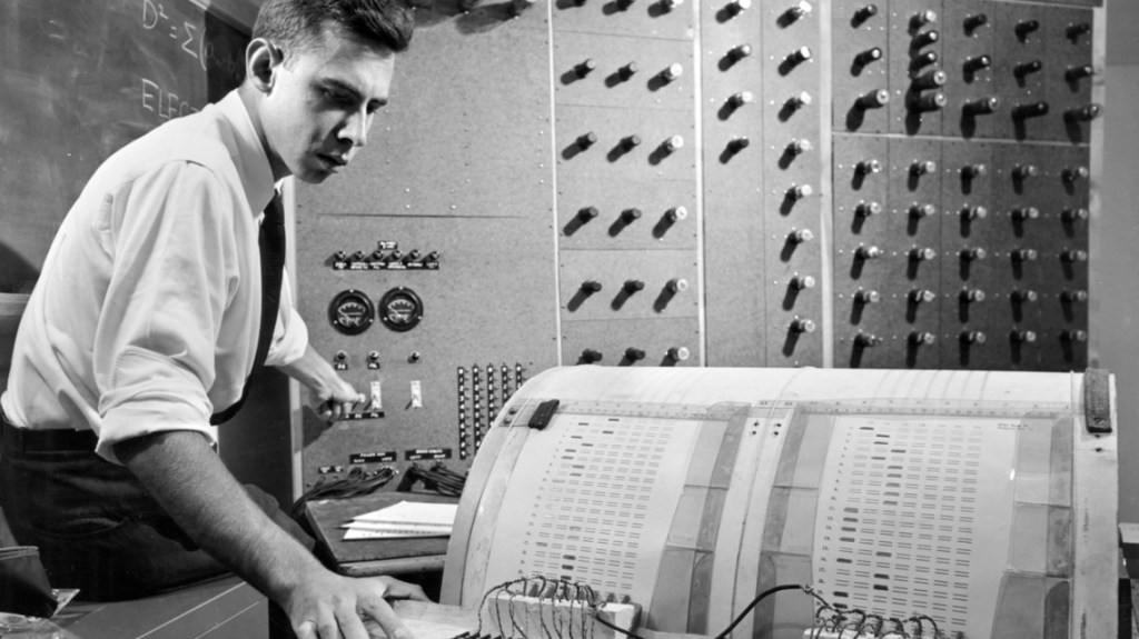
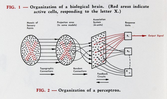
A decade later, during the Cold War, it became necessary to find hidden objects in large numbers of photographs. The embryonic electronic digital computers of the day were far too slow with far too little memory to do the task, so the Navy contracted with the Cornell Aeronautical Laboratory in Cheektowaga, New York, a suburb of Buffalo, to create an analog computer capable of real-time image analysis. This led to the invention of the Perceptron by Frank Rosenblatt as the first neural network-inspired computer [1], building on ideas of neural logic developed by Warren McColloch and Walter Pitts.
Several decades passed with fits and starts as neural networks remained too simple to accomplish anything profound. Then in 1986, David Rumelhart and Ronald Williams at UC San Diego with Geoff Hinton at Carnegie-Mellon discovered a way to train multiple layers of neurons, in a process called error back propagation [2]. This publication opened the floodgates of Connectionism — also known as Parallel Distributed Processing. The late 80’s and much of the 90’s saw an expansion of interest in neural networks, until the increasing size of the networks ran into limits caused by the processing speed and capacity of conventional computers towards the end of the decade. During this time it had become clear that the most interesting computations required many layers of many neurons, and the number of neurons expanded into the thousands, but it was difficult to train such systems that had tens of thousands of adjustable parameters, and research in neural networks once again went into a lull.
The beginnings of deep learning started with two breakthroughs. The first was by Yann Lecun at Bell Labs in 1998 who developed, with Leon Bottou, Yoshua Bengio and Patrick Haffner, a Convolutional Neural Network that had seven layers of neurons that classified hand-written digits [3]. The second was from Geoff Hinton in 2006, by then at the University of Toronto, who discovered a fast learning algorithm for training deep layers of neurons [4]. By the mid 2010’s, research on neural networks was hotter than ever, propelled in part by several very public successes, such as Deep Mind’s machine that beat the best player in the world at Go in 2017, self-driving cars, personal assistants like Siri and Alexa, and YouTube recommendations.
The Challenges of Deep Learning
Deep learning today is characterized by neural network architectures composed of many layers of many neurons. The nature of deep learning brings with it two main challenges: 1) efficient training of the neural weights, and 2) generalization of trained networks to perform accurately on previously unseen data inputs.
Solutions to the first challenge, efficient training, are what allowed the deep revolution in the first place—the result of a combination of increasing computer power with improvements in numerical optimization. This included faster personal computers that allowed nonspecialists to work with deep network programming environments like Matlab’s Deep Learning toolbox and Python’s TensorFlow.
Solutions to the second challenge, generalization, rely heavily on a process known as “regularization”. The term “regularization” has a slippery definition, an obscure history, and an awkward sound to it. Regularization is the noun form of the verb “to regularize” or “to make regular”. Originally, regularization was used to keep certain inverse algorithms from blowing up, like inverse convolutions, also known as deconvolution. Direct convolution is a simple mathematical procedure that “blurs” ideal data based on the natural response of a measuring system. However, if one has experimental data, one might want to deconvolve the system response from the data to recover the ideal data. But this procedure is numerically unstable and can “blow up”, often because of the divide-by-zero problem. Regularization was a simple technique that kept denominators from going to zero.
Regularization became a common method for inverse problems that are notorious to solve because of the many-to-one mapping that can occur in measurement systems. There can be a number of possible causes that produce a single response. Regularization was a way of winnowing out “unphysical” solutions so that the physical inverse solution remained.
During the same time, regularization became a common tool used by quantum field theorists to prevent certain calculated quantities from diverging to infinity. The solution was again to keep denominators from going to zero by setting physical cut-off lengths on the calculations. These cut-offs were initially ad hoc, but the development of renormalization group theory by Kenneth Wilson at Cornell (Nobel Prize in 1982) provided a systematic approach to solving the infinities of quantum field theory.
With the advent of neural networks, having hundreds to thousands to millions of adjustable parameters, regularization became the catch-all term for fighting the problem of over-fitting. Over-fitting occurs when there are so many adjustable parameters that any training data can be fit, and the neural network becomes just a look-up table. Look-up tables are the ultimate hash code, but they have no predictive capability. If a slightly different set of data are fed into the network, the output can be anything. In over-fitting, there is no generalization, the network simply learns the idiosyncrasies of the training data without “learning” the deeper trends or patterns that would allow it to generalize to handle different inputs.
Over the past decades a wide collection of techniques have been developed to reduce over-fitting of neural networks. These techniques include early stopping, k-fold holdout, drop-out, L1 and L2 weight-constraint regularization, as well as physics-based constraints. The goal of all of these techniques is to keep neural nets from creating look-up tables and instead learning the deep codependencies that exist within complicated data.
Table II. Regularization Techniques in Machine Learning
By judicious application of these techniques, combined with appropriate choices of network design, amazingly complex problems can be solved by deep networks and they can generalized too (to some degree). As the field moves forward, we may expect additional regularization tricks to improve generalization, and design principles will emerge so that the networks no longer need to be constructed by trial and error.
The Potential of Deep Learning
In conventional machine learning, one of the most critical first steps performed on a dataset has been feature extraction. This step is complicated and difficult, especially when the signal is buried either in noise or in confounding factors (also known as distractors). The analysis is often highly sensitive to the choice of features, and the selected features may not even be the right ones, leading to bad generalization. In deep learning, feature extraction disappears into the net itself. Optimizing the neural weights subject to appropriate constraints forces the network to find where the relevant information lies and what to do with it.
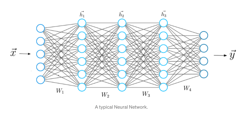
The key to finding the right information was not just having many neurons, but having many layers, which is where the potential of deep learning emerges. It is as if each successive layer is learning a more abstract or more generalized form of the information than the last. This hierarchical layering is most evident in the construction of convolutional deep networks, where the layers are receiving a telescoping succession of information fields from lower levels. Geoff Hinton‘s Deep Belief Network, which launched the deep revolution in 2006, worked explicitly with this hierarchy in mind through direct design of the network architecture. Since then, network architecture has become more generalized, with less up-front design while relying on the increasingly sophisticated optimization techniques of training to set the neural weights. For instance, a simplified instance of a deep network is shown in Fig. 4 with three hidden layers of neurons.
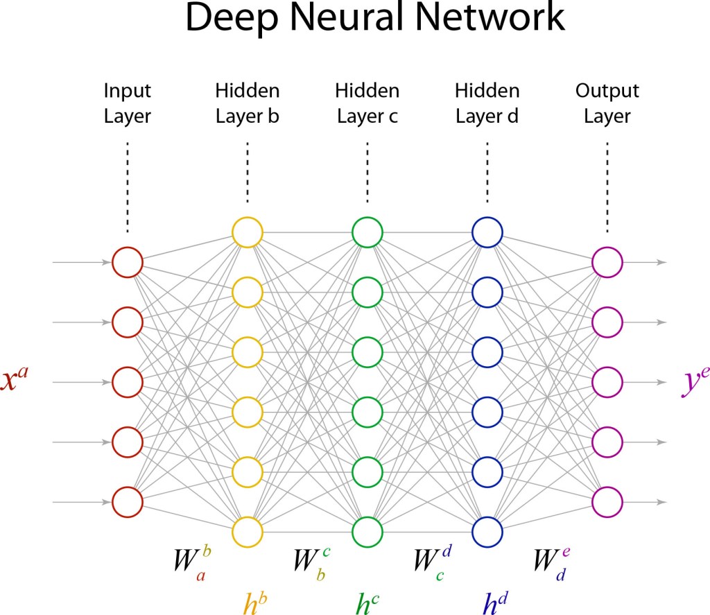
The mathematical structure of a deep network is surprisingly simple. The equations for the network in Fig. 4, that convert an input xa to an output ye, are
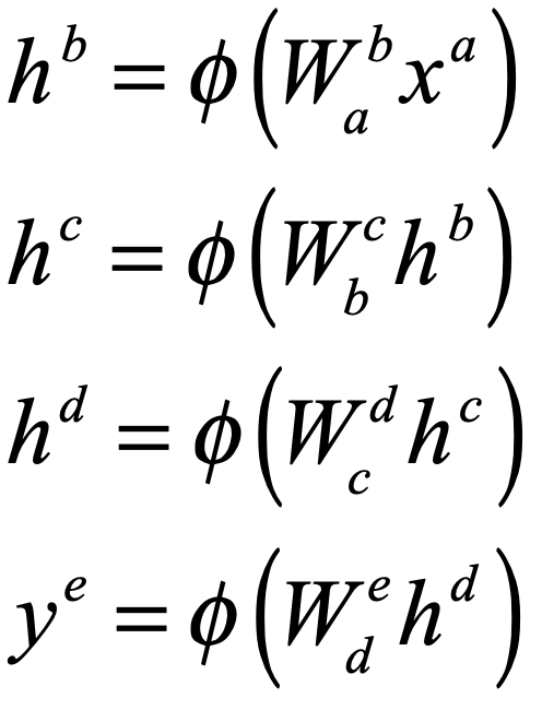
These equations use index notation to denote vectors (single superscript) and matrices (double indexes). The repeated index (one up and one down) denotes an implicit “Einstein” summation. The function φ(.) is known as the activation function, which is nonlinear. One of the simplest activation functions to use and analyze, and the current favorite, is known as the ReLU (for rectifying linear unit). Note that these equations represent a simple neural cascade, as the output of one layer becomes the input for the next.
The training of all the matrix elements assumes a surprisingly simply optimization function, known as an objective function or a loss function, that can look like
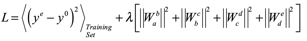
where the first term is the mean squared error of the network output ye relative to the desired output y0 for the training set, and the second term, known as a regularization term (see section above) is a quadratic form that keeps the weights from blowing up. This loss function is minimized over the set of adjustable matrix weights.
The network in Fig. 4 is just a toy, with only 5 inputs and 5 outputs and only 23 neurons. But it has 30+36+36+30+23 = 155 adjustable weights. If this seems like overkill, but it is nothing compared to neural networks with thousands of neurons per layer and tens of layers. That massive overkill is exactly the power of deep learning — as well as its pitfall.
The Pitfalls of Deep Learning
Despite the impressive advances in deep learning, serious pitfalls remain for practitioners. One of the most challenging problems in deep learning is the saddle-point problem. A saddle-point in an objective function is like a mountain pass through the mountains: at the top of the pass it slopes downward in two opposite directions into the valleys but slopes upward in the two orthogonal directions to mountain peaks. A saddle point is an unstable equilibrium where a slight push this way or that can lead the traveller to two very different valleys separated by high mountain ridges. In our familiar three-dimensional space, saddle points are relatively rare and landscapes are dominated by valleys and mountaintops. But this intuition about landscapes fails in high dimensions.
Landscapes in high dimensions are dominated by neutral ridges that span the domain of the landscape. This key understanding about high-dimensional space actually came from the theory of evolutionary dynamics for the evolution of species. In the early days of evolutionary dynamics, there was a serious challenge to understand how genetic mutations could allow such diverse speciation to occur. If the fitness of a species were viewed as a fitness landscape, and if a highly-adapted species were viewed as a mountain peak in this landscape, then genetic mutations would need to drive the population state point into “valleys of death” that would need to be crossed to arrive at a neighboring fitness peak. It would seem that genetic mutations would likely kill off the species in the valleys before they could rise to the next equilibrium.
However, the geometry of high dimensions does not follow this simple low-dimensional intuition. As more dimensions come available, landscapes have more and more ridges of relatively constant height that span the full space (See my recent blog on random walks in 10-dimensions and my short YouTube video). For a species to move from one fitness peak to another fitness peak in a fitness landscape (in ultra-high-dimensional mutation space), all that is needed is for a genetic mutation to step the species off of the fitness peak onto a neutral ridge where many mutations can keep the species on that ridge as it moves ever farther away from the last fitness peak. Eventually, the neutral ridge brings the species near a new fitness peak where it can climb to the top, creating a new stable species. The point is that most genetic mutations are neutral — they do not impact the survivability of an individual. This is known as the neutral network theory of evolution proposed by Motoo Kimura (1924 – 1994) [5]. As these mutation accumulate, the offspring can get genetically far from the progenitor. And when a new fitness peak comes near, many of the previously neutral mutations can come together and become a positive contribution to fitness as the species climbs the new fitness peak.
The neutral network of genetic mutation was a paradigm shift in the field of evolutionary dynamics, and it also taught everyone how different random walks in high-dimensional spaces are from random walks in 3D. But although neutral networks solved the evolution problem, they become a two-edged sword in machine learning. On the positive side, fitness peaks are just like the minima of objective functions, and the ability for partial solutions to perform random walks along neutral ridges in the objective-function space allows optimal solutions to be found across a broad range of the configuration space of the neural weights. However, on the negative side, ridges are loci of unstable equilibrium. Hence there are always multiple directions that a solution state can go to minimize the objective function. Each successive run of a deep-network neural weight optimizer can find equivalent optimal solutions — but they each can be radically different. There is no hope of averaging the weights of an ensemble of networks to arrive at an “average” deep network. The averaging would simply drive all weights to zero. Certainly, the predictions of an ensemble of equivalently trained networks can be averaged—but this does not illuminate what is happening “under the hood” of the machine, which is where our own “understanding” of what the network is doing would come from.
Post-Modern Machine Learning
Post-modernism is admittedly kind of a joke — it works so hard to pull down every aspect of human endeavor that it falls victim to its own methods. The convoluted arguments made by its proponents sound like ultimate slacker talk — circuitous logic circling itself in an endless loop of denial.
But post-modernism does have its merits. It surfs on the moving crest of what passes as modernism, as modernism passes onward to its next phase. The philosophy of post-modernism moves beyond rationality in favor of a subjectivism in which cause and effect are blurred. For instance, in post-modern semiotic theory, a text or a picture is no longer an objective element of reality, but fragments into multiple semiotic versions, each one different for each different reader or watcher — a spectrum of collaborative efforts between each consumer and the artist. The reader brings with them a unique set of life experiences that interact with the text to create an entirely new experience in each reader’s mind.
Deep learning is post-modern in the sense that deterministic algorithms have disappeared. Instead of a traceable path of sequential operations, neural nets scramble information into massively-parallel strings of partial information that cross and interact nonlinearly with other massively-parallel strings. It is difficult to impossible to trace any definable part of the information from input to output. The output simply manifests some aspect of the data that was hidden from human view.
But the Age of Artificial Intelligence is not here yet. The vast multiplicity of saddle ridges in high dimensions is one of the drivers for one of the biggest pitfalls of deep learning — the need for massive amounts of training data. Because there are so many adjustable parameters in a neural network, and hence so many dimensions, a tremendous amount of training data is required to train a network to convergence. This aspect of deep learning stands in strong contrast to human children who can be shown a single picture of a bicycle next to a tricycle, and then they can achieve almost perfect classification accuracy when shown any number of photographs of different bicycles and tricycles. Humans can generalize with an amazingly small amount of data, while deep networks often need thousands of examples. This example alone points to the marked difference between human intelligence and the current state of deep learning. There is still a long road ahead.
By David D. Nolte, April 18, 2022
[1] F. Rosenblatt, “THE PERCEPTRON – A PROBABILISTIC MODEL FOR INFORMATION-STORAGE AND ORGANIZATION IN THE BRAIN,” Psychological Review, vol. 65, no. 6, pp. 386-408, (1958)
[2] D. E. Rumelhart, G. E. Hinton, and R. J. Williams, “LEARNING REPRESENTATIONS BY BACK-PROPAGATING ERRORS,” Nature, vol. 323, no. 6088, pp. 533-536, Oct (1986)
[3] LeCun, Yann; Léon Bottou; Yoshua Bengio; Patrick Haffner (1998). “Gradient-based learning applied to document recognition”. Proceedings of the IEEE. 86 (11): 2278–2324.
[4] G. E. Hinton, S. Osindero, and Y. W. Teh, “A fast learning algorithm for deep belief nets,” Neural Computation, vol. 18, no. 7, pp. 1527-1554, Jul (2006)
[5] M. Kimura, The Neutral Theory of Molecular Evolution. Cambridge University Press, 1968.
