Our century is now a quarter complete, from Y2K to today (2000 – 2025). What have been the greatest discoveries in Physics so far? And what do they portend for the rest of the century?
Every century of physics tends to have its own character:
• The 1600’s were the time of Galileo, Descartes, Huygens, Leibniz and Newton who created the science of dynamics out of nothing.
• The 1700’s were the time of du Chatelet, Maupertuis, Euler, Lagrange, and D’Alembert who constructed mathematical physics on the foundation of the calculus.
• The 1800’s were the time of Young, Fresnel, Hamilton, Maxwell, Boltzmann, and Lord Kelvin who completed the program of classical physics.
• The 1900’s were the time of Einstein and Bohr who invented relativistic and quantum physics and launched the grand program of unified forces.
Now we come to the 2000’s. What will this century be known for?
Two topics physicists have at the top of their mind today is Quantum and AI (and there is even quantum AI). But AI is merely a tool (though an important one that is radically changing how physics is done), and quantum is a catch-all (almost everything is quantum at its core).
So, what are the greatest breakthroughs of the 21st Century so far? And what do they portend for the eventual “character” of 21st-Century physics when seen in the rear-view mirror of history by the year 2100?
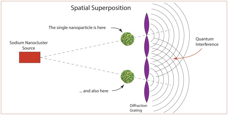
Single-photon Quantum Information (2001)
The century started on July 24, 2000, when a landmark paper was received by Nature magazine submitted by Emanuel Knill and Raymond Laflamme at Los Alamos National Lab in the United States with Gerald Milburn from the University of Queensland, Australia (collectively known as KLM). This little-heralded paper proposed a radical new idea in quantum information, an idea that would have profound effects on the development of quantum science for the coming quarter-century.
The idea was simply that quantum logic could be performed with single photons and linear optics [1]. Up to that point, most research on quantum optical computing was trying to get photons to interact with each other (which they really don’t like to do) in nonlinear media like crystals or trapped atoms. What KLM showed was that quantum information could be manipulated in general ways without interactions. The paper proposed a technique that could perform quantum logic in a universal way using only linear optical elements like single-photon sources, beam splitters, phase shifters, and single-photon detectors, introducing the novel idea of “measurement-based” quantum computing.
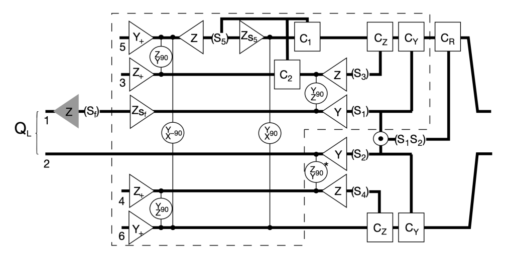
In the quarter-century since the publication of the KLM paper, LOQC has steadily progressed via the development of single-photon sources and detectors. Today, numerous start-ups are pursuing LOQC, notably Xanadu in Toronto, Canada, and PsiQuantum in Palo Alto, USA and Brisbane, Australia. By 2100, this century will likely be viewed as the time when applications of quantum information reached their maturity. Where the 20th century was a century of discovery of quantum phenomena, the 21st will be the century when it was reduced to practice.
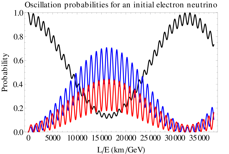
Solar Neutrino Oscillation (2001)
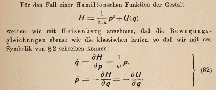
The sun is fueled by the fusion of hydrogen that generates electron neutrinos. The reaction looks like
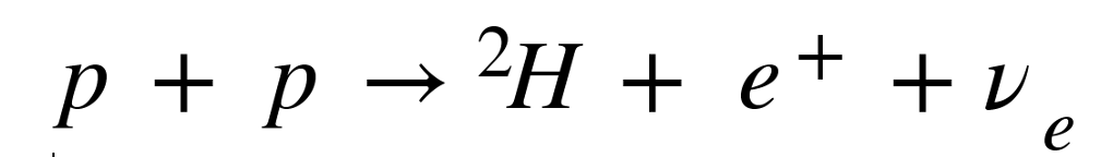
where p is a proton (hydrogen), 2H is deuterium (a hydrogen nucleus with an extra neutron), e+ is a positron (the anti-matter form of an electron) and ν e is an electron neutrino. This reaction accounts for 99% of the neutrinos generated by the Sun, calculated by the theoretical astrophysicist John Bahcall of the Institute for Advanced Study at Princeton University. Already by the late 1960’s it was suspected that too few of the neutrinos were being detected compared to predictions, so he teamed with Raymond Davis of Brookhaven National Lab to build an experiment to detect the flux of solar neutrinos. To shield the detector from cosmic rays, the experiment was placed at the 4850 level of the Homestake Gold Mine in Lead, South Dakota and operated from 1970 to 1994. The deficit of solar neutrinos was confirmed, and it was huge: Fully two-thirds of expected solar neutrinos were missing!
The simplest solution to the missing solar neutrinos was that they just weren’t there because, on their way to Earth from the Sun, they had converted to something else that was not detectedable. This conversion from one particle to another is possible if neutrinos have a non-zero (but extremely small) mass. If so, then an electron neutrino can convert to a muon neutrino, and if the distance is far enough, they can convert back. In other words, the nature of the neutrino particle is that its identity oscillates. This is called the solar neutrino oscillation, and by the time the neutrinos have arrived at Earth, two-thirds of them have converted to muon neutrinos.
There was a general reluctance to accept neutrino oscillations because it represented a departure from the Standard Model of particle physics and introduced uncomfortably small masses for neutrinos that otherwise behave like massless particles. Two experiments put these qualms to rest: the Super-Kamiokanda expeeriment in Japan and the Sudbury Neutrino Oscillation experiment in Canada. By the early years of the century, neutrino oscillations had been confirmed.
By 2100, the mystery of the ultra-small neutrino masses will likely have been solved. If the answer falls within the Standard Model, then this may be the crowning achievement that “completes” the standard model. If the answer falls outside the Standard Model, then this may be the beginning of a new chapter in high-energy physics.
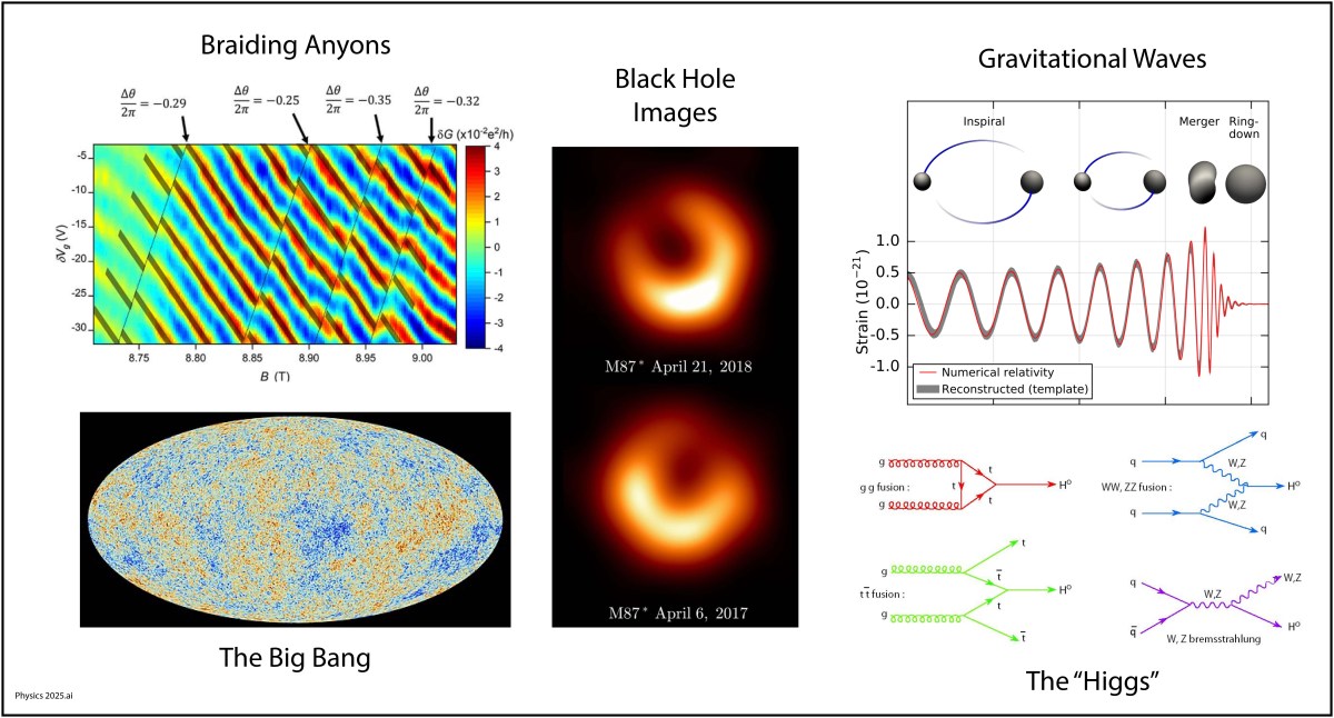
WMAP and Planck (2003)
The Big Bang may have occurred 13.7 billion years ago, but that Bang echoes to this day across the Universe. At its inception, the reverberations were incredibly hot, but they have cooled now to a mere 3 degrees Kelvin. In 1987, Paul Richards and Andrew Lange at the University of California at Berkeley, recorded the peak of the Planck black body spectrum during a sounding rocket flight that carried a far-infrared spectrometer to the edge of space. (The dichroic bandpass filters in their spectrometer were the first far-infrared metamaterials. I designed and built them as a young grad student at Berkeley! [2]) This experiment was followed by the COBE satellite that measured the presence of minuscule fluctuations in the temperature, representing the original heterogeneity of the universe just after the Big Bang.
COBE flew for a year, followed in 1998 by the BOOMerAng experiment, led by Andrew Lange, that was suspended from a high-altitude balloon circling the South Pole for ten days. This experiment discovered the literal echoes of the Big Bang, acoustic oscillations, in other words, the “sound” of the Bang. It also established that the universe is gravitationally “flat”, which is a direct consequence of cosmic inflation. Once again, these findings were followed by a satellite experiment, the WMAP mission in 2003, that mapped these oscillations over the entire sky. Even finer resolution was obtained by the Planck mission in 2013, measuring higher harmonics of the sound oscillations. These oscillations in the early universe helped seed regions of slightly higher density that condensed into galaxies, leading to the large-scale structure of the universe that we see today.
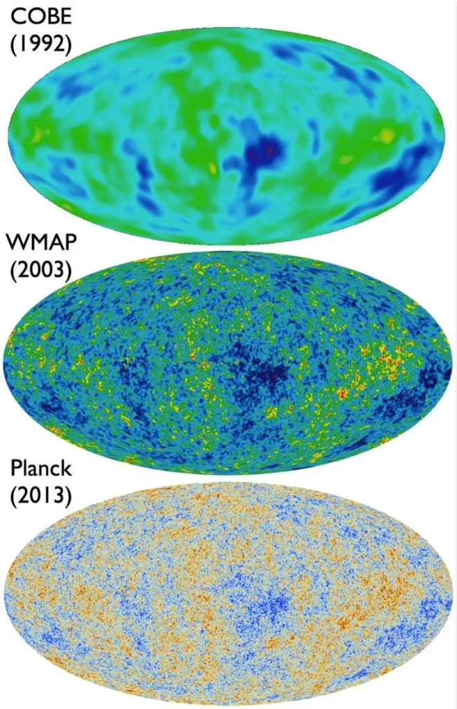
The 21st Century will likely be known as the time when the physics of the early universe was finally pinned down, and maybe even of what can before. The answers may tell us if there are parallel universes in a much larger metaverse.
Exoplanets (2009)
The Earth is not alone in the Universe. It is not even alone in our little neighborhood of the Milky Way. Within 50 light years it is estimated that there are about 1000 Earth-sized planets in the habitable zone of their respective stars. Why is 50 light years significant? It is because, within this century, the technology to explore those planets is likely to be developed. With the right designs, an unmanned probe could reach 50 light years from Earth within a century, and the time to call back home is only 50 years. So if a probe is launched in the year 2100, we could be receiving transmissions from the new planet by the year 2250.
This estimate of 1000 New Earths is the result of a quiet revolution in planetary science that has been unfolding over the past quarter century. The very first exoplanet was confirmed in 1995 by Michel Mayor and Didier Queloz. Today, as of the writing of this blog, there are 6,278 confirmed exoplanets. Most of these were disovered by the Kepler satellite that was launched in 2009.
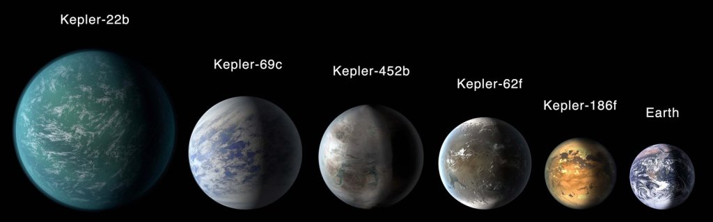
By 2100, we will know where all the exoplanets are that are within 50 light years of Earth, and we will know which ones are potential inhabitable. It may even happen that signs of life on one of these planets will have been discovered. If so, then it is hard to imagine humankind NOT launching probes to visit those planets. If the right propulsion technology is developed, then those probes could be signaling back information from those planets as early as the year 2250…if anyone is still here to listen.
The Higgs (2012)
The crowning achievement of high-energy physics may also have been the last nail in the coffin. Throughout the second half of the 20th century, high-energy physics took the lion’s share of money and attention showered on physics. Beginning in the aftermath of the Manhattan Project, the search for the fundamental constituents of our universe at first found more and more particles, creating a “zoo” that resisted easy classification, until quarks were proposed that simplified the whole thing down into what is now called the Standard Model of Physics.
But one piece of the puzzle was still missing–the explanation of why particles have the masses they do. This missing piece was supplied by the theoretical physicist Peter Higgs in 1964 who proposed that point-like massless particles interacted with a “field” that permeated space. The interaction energy was equivalent to mass through Einstein’s famous E = mc2, and the quantization of the field predicted the existence of a “Higgs Boson”. The search for the “Higgs”, as it is called for short, became the Holy Grail of Physics at the end of the last century.
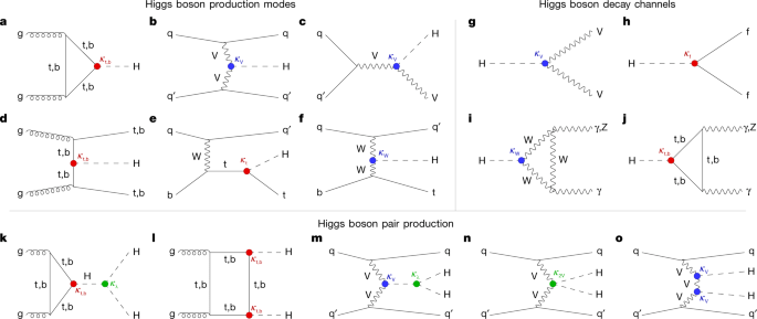
The discovery of the Higgs boson was announced on the 4th of July in 2012 [3]. It capped 80 years of progress in high-energy particle physics since the discovery of the positron in 1932. But it may also be the last. Since 2012, over the past 14 years, there have been no new “major” discoveries at the Large Hadron Collider (LHC). Most high-energy talks since then have been about speculative experiments seeking deviations from the Standard Model, but so far there is nothing new.
In the year 2100, looking back, the era of high-energy physics may be relegated to the 20th century, with the Higgs just a finishing touch that tipped over into the new millennium … Or sometime in the next 75 years there will be a discovery that goes beyond standard physics and opens a new chapter in the field. We will have to wait to see.
Gravitational Waves (2015)
Where were you on Nov. 11, 2015 at 10:30 am? Can you remember? I can! I was in a conference room in the Physics Building on the Purdue University Campus waiting with a small crowd of physicists for a news conference to begin. Everyone knew it would be something big. It was. They announced the first detection of a gravitational wave by the LIGO detector (the Laser Interferometric Gravitational Wave Observatory). In a way, it was anti-climactic because we all knew that LIGO would eventually see one. But it was also immensely dramatic, because it was the most sensitive measurement ever made by mankind. The displacement of the mirrors in the interferometer caused by the passing gravitational wave was a tiny fraction of a radius of a proton, yet the signal was as clear as a bell. It came from the merger of two 30 solar-mass black holes in a galaxy far, far away.
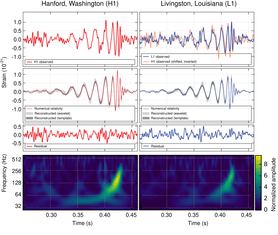
By the year 2100, looking back, multi-messenger astronomy will have been a key part of the physics of the 21st century. Multi-messenger astronomy is when an astronomical event is detected across many detection modes, possibly including light, infrared, ultraviolet, x-ray, neutrino and gravitational wave detection. The field is just beginning and has a long way to go to integrate all these different ways of seeing into a complete picture of what happens out in the universe.
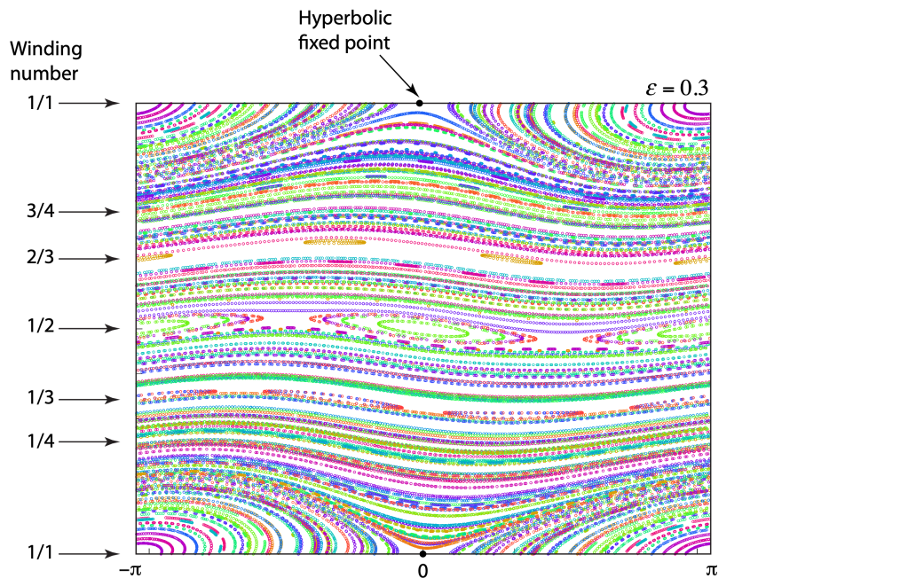
Topological physics (2016)
Of all the topics of this blog, this one is perhaps the most abstract. When we think of geometry, it is natural to think in terms of the symmetries that objects have. The last century was the pinnacle of geometric physics, where Einstein showed that gravity is a geometric property of warped space, where group theory classified all the ways that objects can be constructed and behave, and symmetry breaking was invoked to explain the hierarchy of physical forces.
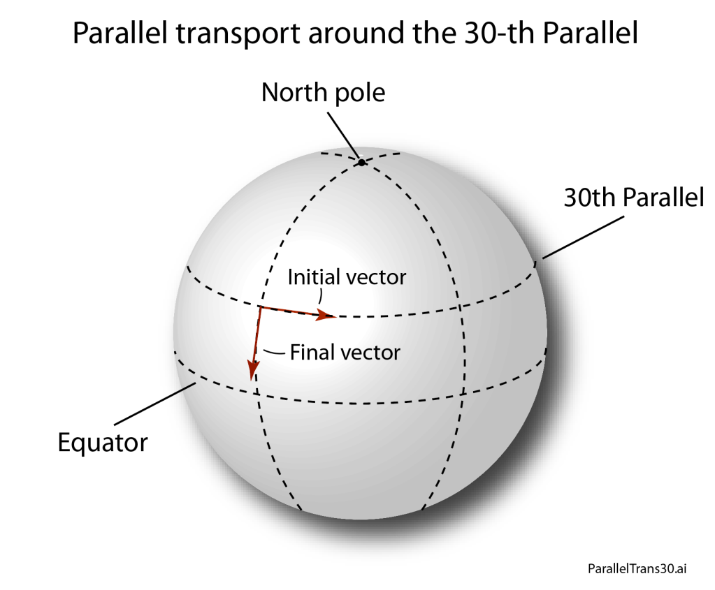
The new century will be the time of topological physics, where symmetries of matter may not even matter, but the way that properties of matter are connected does. By “property of matter” I mean like the electronic states of a solid state material where the states are excluded from portions of state space, creating topology in abstract spaces. Such topological properties govern how freely currents can flow on surfaces but not in the bulk, or vice versa. In quantum systems, topological properties can protect quantum information from decoherence, which is the bane of most real-world implementations of quantum computers. For instance, by “braiding anyons” it is possible to create qubits that resist dephasing.
The importance of topology in physics was recognized with the 2016 Nobel Prize to David J. Thouless, F. Duncan M. Haldane, and J. Michael Kosterlitz for “Theoretical discoveries of topological phase transitions and topological phases of matter.”
Images of Black Holes (2019)
Why hasn’t this gotten a Nobel Prize yet? The imaging of black holes is a tour de force, requiring a telescope with the diameter of a planet, and requiring the collaboration of scientists from across that planet to make it all work.
The physics is straightforward. Everyone knows that bigger telescopes have better resolution, so the logical limit is a telescope the size of the Earth. This is accomplished by using interferometric detection, with data from widely spread millimeter-wave telescopes synchronized by an atomic clock in a network of telescopes known as the Event Horizon Telescope (EHT). The results are constructed numerically, as shown below.
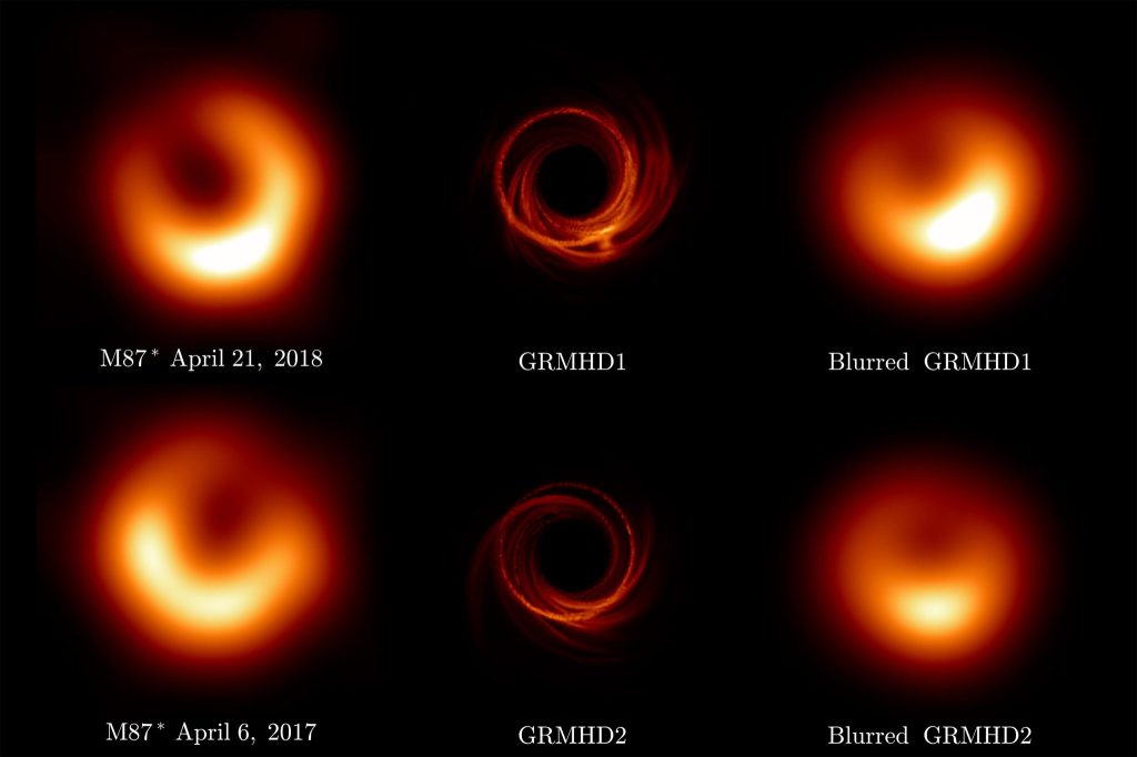
Fig. 7. The EHT images (left) compared to the model (middle) and the blurred model (right) of the black hole in the M87 galaxy. From Ref.
The next logical step for this kind of imaging is a telescope array that is bigger than the Earth … much bigger! This could be accomplished with an array of Lagrange-point satellites, improving the resolution of the images. By the end of this century, we may be imaging the black holes in all the near-by galaxies.
More to Come?
What are the greatest outstanding problems of physics that may yet yield to solutions within this century? It is impossible to say for certain without a crystal ball, but there are some that are likely to be resolved in the next 75 years:
• Dark Matter: This is the 500 pound gorilla in the room. If most of the tangible universe is made of this stuff, then we had better get around to detecting it!
• Dark Energy: This is the other 500 pound gorilla in the room. If most of the intangible universe is made of this stuff, then we had better get a good understanding of it.
• Quantum Gravity: Of the four forces of physics (gravity, electro-magnetic, weak nuclear and strong nuclear) gravity stands apart in several ways, one of which is that there is no quantum theory for it. We have 75 years to fix this if it is to be a crowning achievement of 21st-Century physics.
• The Evolution of Life: I didn’t include any biophysics in my list of the best physics of the century mainly because I cannot point to a single revolutionary breakthrough of physics in this area. There has been a lot of good progress on the microphysics of biological systems, but nothing like discovering a Higgs boson. This could change if the origins of life turn out to be physics-based rather than just some chemistry.
• The Evolution of Intelligence: I think physics has more to say on the evolution of intelligence than on the evolution of life. Intelligence is the quintessential complex system, and the methods of theoretical physics may yet provide a clear answer to the question of “What is Intelligence?”.
• The Early Universe: This is just starting now with the James Webb Telescope peering into the dark depths of history–nearly to the Big Bang itself.
• Multiple Dimensions: String theory likes to live in 11-dimensional space, so what other parts of our physical universe live there too? Dark Matter? Dark Energy? Do all the extra dimensions need to be compact?
• The Arrow of Time: The physics of time is possibly the greatest unsolved problem in physics. Why does it only go one way?
• Singularity Physics: What happens at the center of a Black Hole? Do wormholes provide hyperspace bypasses? These questions may yet get answers from theoretical physics though likely not from the laboratory unless it is from an AMO analog.
References
[1] E. Knill, R. Laflamme and G. J. Milburn, A Scheme for Efficient Quantum Computation with Linear Optics, Nature 409 (6816), 46–52 (2001).
[2] D. NOLTE, A. LANGE and P. RICHARDS, Far-Infrared Dichroic Bandpass-Filters, Applied Optics 24 (10), 1541–1545 (1985).
[3] CERN. (2012, July 4). CERN experiments observe particle consistent with long-sought Higgs boson [Press release]. https://home.cern/news/press-release/cern/cern-experiments-observe-particle-consistent-long-sought-higgs-boson; ATLAS Collaboration. (2012). Observation of a new particle in the search for the Standard Model Higgs boson with the ATLAS detector at the LHC. Physics Letters B, 716(1), 1–29. https://doi.org/10.1016/j.physletb.2012.08.020 Cited by: 13000+; CMS Collaboration. (2012). Observation of a new boson at a mass of 125 GeV with the CMS experiment at the LHC. Physics Letters B, 716(1), 30–61. https://doi.org/10.1016/j.physletb.2012.08.021