Chaos seems to rule our world. Weather events, natural disasters, economic volatility, empire building—all these contribute to the complexities that buffet our lives. It is no wonder that ancient man attributed the chaos to the gods or to the fates, infinitely far from anything we can comprehend as cause and effect. Yet there is a balm to soothe our wounds from the slings of life—Chaos Theory—if not to solve our problems, then at least to understand them.
Chaos Theory is the theory of complex systems governed by multiple factors that produce complicated outputs. The power of the theory is its ability recognize when the complicated outputs are not “random”, no matter how complicated they are, but are in fact determined by the inputs. Furthermore, chaos theory finds structures and patterns within the output—like the fractal structures known as “strange attractors”. These patterns not only are not random, but they tell us about the internal mechanics of the system, and they tell us where to look “on average” for the system behavior.
In other words, chaos theory tames the chaos, and we no longer need to blame gods or the fates.
Henri Poincare (1889)
The first glimpse of the inner workings of chaos was made by accident when Henri Poincaré responded to a mathematics competition held in honor of the King of Sweden. The challenge was to prove whether the solar system was absolutely stable, or whether there was a danger that one day the Earth would be flung from its orbit. Poincaré had already been thinking about the stability of dynamical systems so he wrote up his solution to the challenge and sent it in, believing that he had indeed proven that the solar system was stable.
from the book Galileo Unbound, (Oxford University Press)
His entry to the competition was the most convincing, so he was awarded the prize and instructed to submit the manuscript for publication. The paper was already at the printers and coming off the presses when Poincaré was asked by the competition organizer to check one last part of the proof which one of the reviewer’s had questioned relating to homoclinic orbits.

To Poincaré’s horror, as he checked his results against the reviewer’s comments, he found that he had made a fundamental error, and in fact the solar system would never be stable. The problem that he had overlooked had to do with the way that orbits can cross above or below each other on successive passes, leading to a tangle of orbital trajectories that crisscrossed each other in a fine mesh. This is known as the “homoclinic tangle”: it was the first glimpse that deterministic systems could lead to unpredictable results. Most importantly, he had developed the first mathematical tools that would be needed to analyze chaotic systems—such as the Poincaré section—but nearly half a century would pass before these tools would be picked up again.
Poincaré paid out of his own pocket for the first printing to be destroyed and for the corrected version of his manuscript to be printed in its place [1]. No-one but the competition organizers and reviewers ever saw his first version. Yet it was when he was correcting his mistake that he stumbled on chaos for the first time, which is what posterity remembers him for. This little episode in the history of physics went undiscovered for a century before being brought to light by Barrow-Green in her 1997 book Poincaré and the Three Body Problem [2].

Cartwight and Littlewood (1945)
During World War II, self-oscillations and nonlinear dynamics became strategic topics for the war effort in England. High-power magnetrons were driving long-range radar, keeping Britain alert to Luftwaffe bombing raids, and the tricky dynamics of these oscillators could be represented as a driven van der Pol oscillator. These oscillators had been studied in the 1920’s by the Dutch physicist Balthasar van der Pol (1889–1959) when he was completing his PhD thesis at the University of Utrecht on the topic of radio transmission through ionized gases. van der Pol had built a short-wave triode oscillator to perform experiments on radio diffraction to compare with his theoretical calculations of radio transmission. Van der Pol’s triode oscillator was an engineering feat that produced the shortest wavelengths of the day, making van der Pol intimately familiar with the operation of the oscillator, and he proposed a general form of differential equation for the triode oscillator.

Research on the radar magnetron led to theoretical work on driven nonlinear oscillators, including the discovery that a driven van der Pol oscillator could break up into wild and intermittent patterns. This “bad” behavior of the oscillator circuit (bad for radar applications) was the first discovery of chaotic behavior in man-made circuits.
These irregular properties of the driven van der Pol equation were studied by Mary- Lucy Cartwright (1990–1998) (the first woman to be elected a fellow of the Royal Society) and John Littlewood (1885–1977) at Cambridge who showed that the coexistence of two periodic solutions implied that discontinuously recurrent motion—in today’s parlance, chaos— could result, which was clearly undesirable for radar applications. The work of Cartwright and Littlewood [3] later inspired the work by Levinson and Smale as they introduced the field of nonlinear dynamics.

Andrey Kolmogorov (1954)
The passing of the Russian dictator Joseph Stalin provided a long-needed opening for Soviet scientists to travel again to international conferences where they could meet with their western colleagues to exchange ideas. Four Russian mathematicians were allowed to attend the 1954 International Congress of Mathematics (ICM) held in Amsterdam, the Netherlands. One of those was Andrey Nikolaevich Kolmogorov (1903 – 1987) who was asked to give the closing plenary speech. Despite the isolation of Russia during the Soviet years before World War II and later during the Cold War, Kolmogorov was internationally renowned as one of the greatest mathematicians of his day.
By 1954, Kolmogorov’s interests had spread into topics in topology, turbulence and logic, but no one was prepared for the topic of his plenary lecture at the ICM in Amsterdam. Kolmogorov spoke on the dusty old topic of Hamiltonian mechanics. He even apologized at the start for speaking on such an old topic when everyone had expected him to speak on probability theory. Yet, in the length of only half an hour he laid out a bold and brilliant outline to a proof that the three-body problem had an infinity of stable orbits. Furthermore, these stable orbits provided impenetrable barriers to the diffusion of chaotic motion across the full phase space of the mechanical system. The crucial consequences of this short talk were lost on almost everyone who attended as they walked away after the lecture, but Kolmogorov had discovered a deep lattice structure that constrained the chaotic dynamics of the solar system.
Kolmogorov’s approach used a result from number theory that provides a measure of how close an irrational number is to a rational one. This is an important question for orbital dynamics, because whenever the ratio of two orbital periods is a ratio of integers, especially when the integers are small, then the two bodies will be in a state of resonance, which was the fundamental source of chaos in Poincaré’s stability analysis of the three-body problem. After Komogorov had boldly presented his results at the ICM of 1954 [4], what remained was the necessary mathematical proof of Kolmogorov’s daring conjecture. This would be provided by one of his students, V. I. Arnold, a decade later. But before the mathematicians could settle the issue, an atmospheric scientist, using one of the first electronic computers, rediscovered Poincaré’s tangle, this time in a simplified model of the atmosphere.
Edward Lorenz (1963)
In 1960, with the help of a friend at MIT, the atmospheric scientist Edward Lorenz purchased a Royal McBee LGP-30 tabletop computer to make calculation of a simplified model he had derived for the weather. The McBee used 113 of the latest miniature vacuum tubes and also had 1450 of the new solid-state diodes made of semiconductors rather than tubes, which helped reduce the size further, as well as reducing heat generation. The McBee had a clock rate of 120 kHz and operated on 31-bit numbers with a 15 kB memory. Under full load it used 1500 Watts of power to run. But even with a computer in hand, the atmospheric equations needed to be simplified to make the calculations tractable. Lorenz simplified the number of atmospheric equations down to twelve, and he began programming his Royal McBee.
Progress was good, and by 1961, he had completed a large initial numerical study. One day, as he was testing his results, he decided to save time by starting the computations midway by using mid-point results from a previous run as initial conditions. He typed in the three-digit numbers from a paper printout and went down the hall for a cup of coffee. When he returned, he looked at the printout of the twelve variables and was disappointed to find that they were not related to the previous full-time run. He immediately suspected a faulty vacuum tube, as often happened. But as he looked closer at the numbers, he realized that, at first, they tracked very well with the original run, but then began to diverge more and more rapidly until they lost all connection with the first-run numbers. The internal numbers of the McBee had a precision of 6 decimal points, but the printer only printed three to save time and paper. His initial conditions were correct to a part in a thousand, but this small error was magnified exponentially as the solution progressed. When he printed out the full six digits (the resolution limit for the machine), and used these as initial conditions, the original trajectory returned. There was no mistake. The McBee was working perfectly.
At this point, Lorenz recalled that he “became rather excited”. He was looking at a complete breakdown of predictability in atmospheric science. If radically different behavior arose from the smallest errors, then no measurements would ever be accurate enough to be useful for long-range forecasting. At a more fundamental level, this was a break with a long-standing tradition in science and engineering that clung to the belief that small differences produced small effects. What Lorenz had discovered, instead, was that the deterministic solution to his 12 equations was exponentially sensitive to initial conditions (known today as SIC).
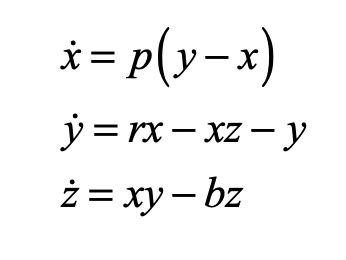
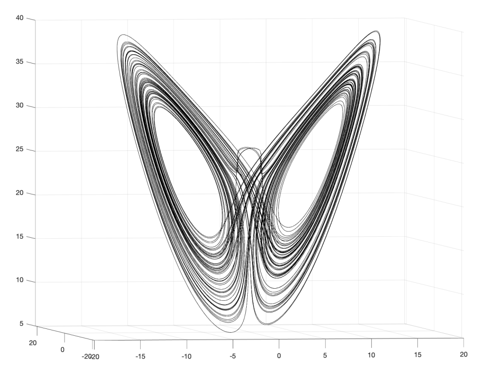
The more Lorenz became familiar with the behavior of his equations, the more he felt that the 12-dimensional trajectories had a repeatable shape. He tried to visualize this shape, to get a sense of its character, but it is difficult to visualize things in twelve dimensions, and progress was slow, so he simplified his equations even further to three variables that could be represented in a three-dimensional graph [5].

V. I. Arnold (1964)
Meanwhile, back in Moscow, an energetic and creative young mathematics student knocked on Kolmogorov’s door looking for an advisor for his undergraduate thesis. The youth was Vladimir Igorevich Arnold (1937 – 2010), who showed promise, so Kolmogorov took him on as his advisee. They worked on the surprisingly complex properties of the mapping of a circle onto itself, which Arnold filed as his dissertation in 1959. The circle map holds close similarities with the periodic orbits of the planets, and this problem led Arnold down a path that drew tantalizingly close to Kolmogorov’s conjecture on Hamiltonian stability. Arnold continued in his PhD with Kolmogorov, solving Hilbert’s 13th problem by showing that every function of n variables can be represented by continuous functions of a single variable. Arnold was appointed as an assistant in the Faculty of Mechanics and Mathematics at Moscow State University.
Arnold’s habilitation topic was Kolmogorov’s conjecture, and his approach used the same circle map that had played an important role in solving Hilbert’s 13th problem. Kolmogorov neither encouraged nor discouraged Arnold to tackle his conjecture. Arnold was led to it independently by the similarity of the stability problem with the problem of continuous functions. In reference to his shift to this new topic for his habilitation, Arnold stated “The mysterious interrelations between different branches of mathematics with seemingly no connections are still an enigma for me.” [6]
Arnold began with the problem of attracting and repelling fixed points in the circle map and made a fundamental connection to the theory of invariant properties of action-angle variables . These provided a key element in the proof of Kolmogorov’s conjecture. In late 1961, Arnold submitted his results to the leading Soviet physics journal—which promptly rejected it because he used forbidden terms for the journal, such as “theorem” and “proof”, and he had used obscure terminology that would confuse their usual physicist readership, terminology such as “Lesbesgue measure”, “invariant tori” and “Diophantine conditions”. Arnold withdrew the paper.
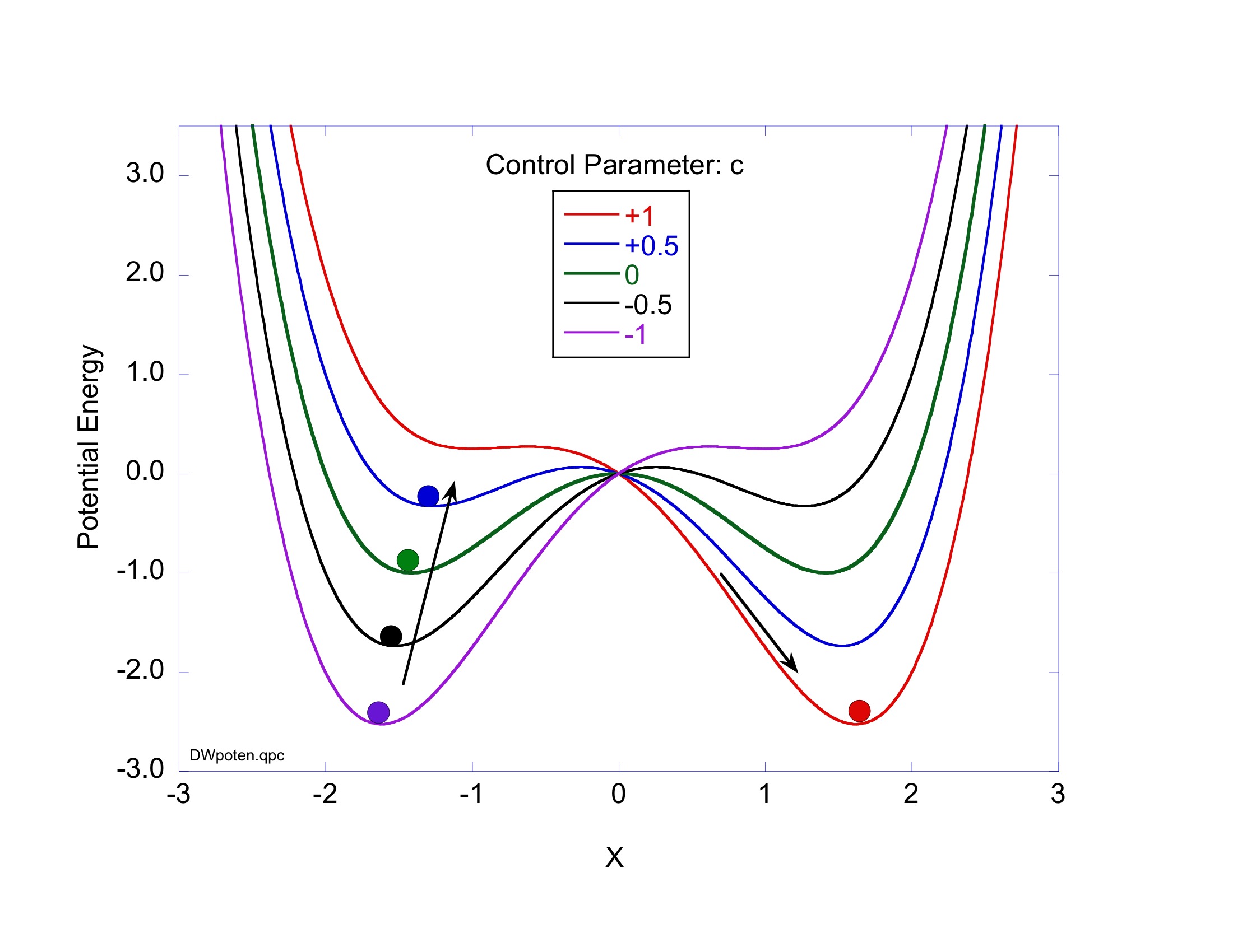
Arnold later incorporated an approach pioneered by Jurgen Moser [7] and published a definitive article on the problem of small divisors in 1963 [8]. The combined work of Kolmogorov, Arnold and Moser had finally established the stability of irrational orbits in the three-body problem, the most irrational and hence most stable orbit having the frequency of the golden mean. The term “KAM theory”, using the first initials of the three theorists, was coined in 1968 by B. V. Chirikov, who also introduced in 1969 what has become known as the Chirikov map (also known as the Standard map ) that reduced the abstract circle maps of Arnold and Moser to simple iterated functions that any student can program easily on a computer to explore KAM invariant tori and the onset of Hamiltonian chaos, as in Fig. 1 [9].

Sephen Smale (1967)
Stephen Smale was at the end of a post-graduate fellowship from the National Science Foundation when he went to Rio to work with Mauricio Peixoto. Smale and Peixoto had met in Princeton in 1960 where Peixoto was working with Solomon Lefschetz (1884 – 1972) who had an interest in oscillators that sustained their oscillations in the absence of a periodic force. For instance, a pendulum clock driven by the steady force of a hanging weight is a self-sustained oscillator. Lefschetz was building on work by the Russian Aleksandr A. Andronov (1901 – 1952) who worked in the secret science city of Gorky in the 1930’s on nonlinear self-oscillations using Poincaré’s first return map. The map converted the continuous trajectories of dynamical systems into discrete numbers, simplifying problems of feedback and control.
The central question of mechanical control systems, even self-oscillating systems, was how to attain stability. By combining approaches of Poincaré and Lyapunov, as well as developing their own techniques, the Gorky school became world leaders in the theory and applications of nonlinear oscillations. Andronov published a seminal textbook in 1937 The Theory of Oscillations with his colleagues Vitt and Khaykin, and Lefschetz had obtained and translated the book into English in 1947, introducing it to the West. When Peixoto returned to Rio, his interest in nonlinear oscillations captured the imagination of Smale even though his main mathematical focus was on problems of topology. On the beach in Rio, Smale had an idea that topology could help prove whether systems had a finite number of periodic points. Peixoto had already proven this for two dimensions, but Smale wanted to find a more general proof for any number of dimensions.
Norman Levinson (1912 – 1975) at MIT became aware of Smale’s interests and sent off a letter to Rio in which he suggested that Smale should look at Levinson’s work on the triode self-oscillator (a van der Pol oscillator), as well as the work of Cartwright and Littlewood who had discovered quasi-periodic behavior hidden within the equations. Smale was puzzled but intrigued by Levinson’s paper that had no drawings or visualization aids, so he started scribbling curves on paper that bent back upon themselves in ways suggested by the van der Pol dynamics. During a visit to Berkeley later that year, he presented his preliminary work, and a colleague suggested that the curves looked like strips that were being stretched and bent into a horseshoe.
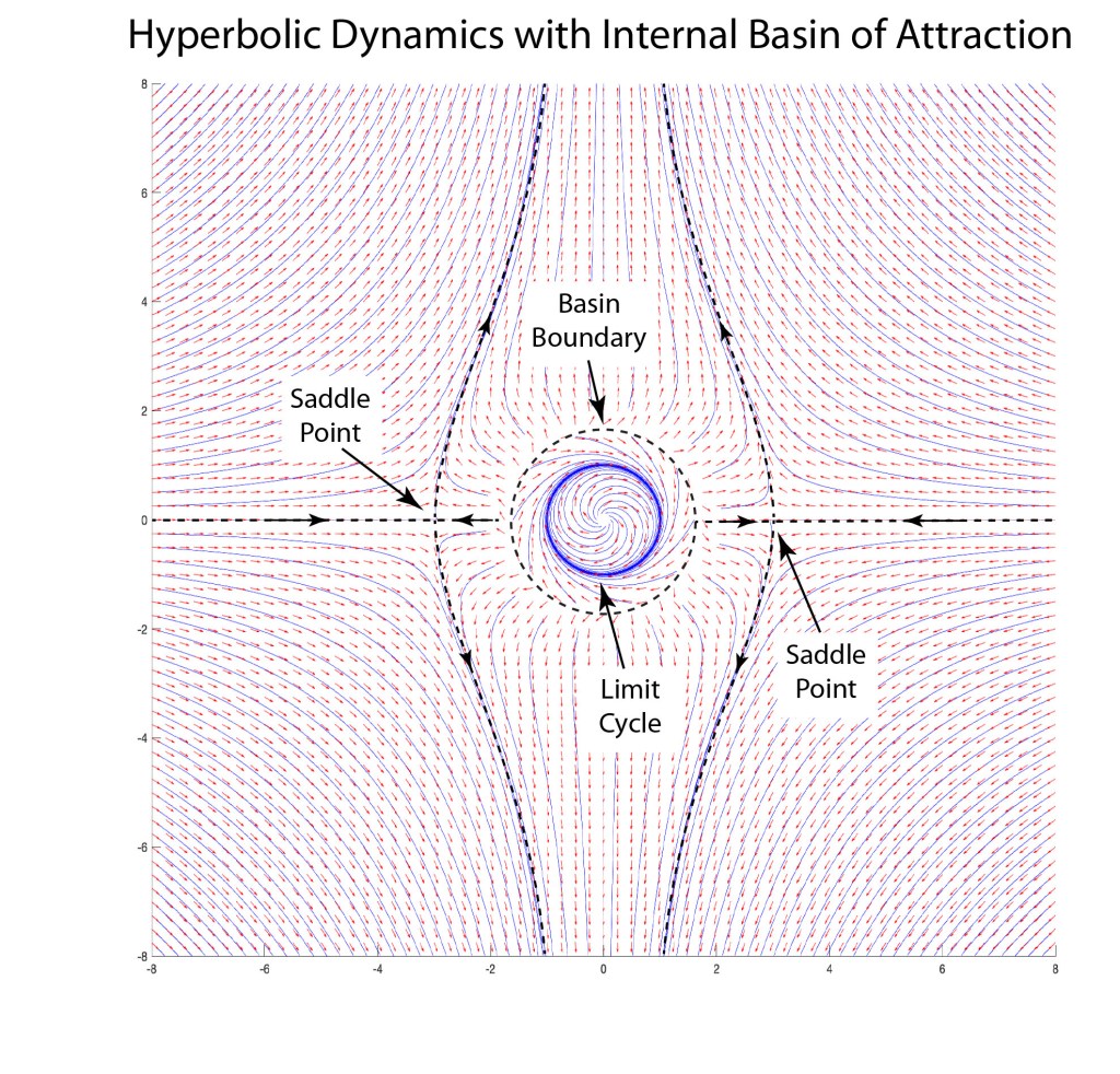
Smale latched onto this idea, realizing that the strips were being successively stretched and folded under the repeated transformation of the dynamical equations. Furthermore, because dynamics can move forward in time as well as backwards, there was a sister set of horseshoes that were crossing the original set at right angles. As the dynamics proceeded, these two sets of horseshoes were repeatedly stretched and folded across each other, creating an infinite latticework of intersections that had the properties of the Cantor set. Here was solid proof that Smale’s original conjecture was wrong—the dynamics had an infinite number of periodicities, and they were nested in self-similar patterns in a latticework of points that map out a Cantor-like set of points. In the two-dimensional case, shown in the figure, the fractal dimension of this lattice is D = ln4/ln3 = 1.26, somewhere in dimensionality between a line and a plane. Smale’s infinitely nested set of periodic points was the same tangle of points that Poincaré had noticed while he was correcting his King Otto Prize manuscript. Smale, using modern principles of topology, was finally able to put rigorous mathematical structure to Poincaré’s homoclinic tangle. Coincidentally, Poincaré had launched the modern field of topology, so in a sense he sowed the seeds to the solution to his own problem.

Ruelle and Takens (1971)
The onset of turbulence was an iconic problem in nonlinear physics with a long history and a long list of famous researchers studying it. As far back as the Renaissance, Leonardo da Vinci had made detailed studies of water cascades, sketching whorls upon whorls in charcoal in his famous notebooks. Heisenberg, oddly, wrote his PhD dissertation on the topic of turbulence even while he was inventing quantum mechanics on the side. Kolmogorov in the 1940’s applied his probabilistic theories to turbulence, and this statistical approach dominated most studies up to the time when David Ruelle and Floris Takens published a paper in 1971 that took a nonlinear dynamics approach to the problem rather than statistical, identifying strange attractors in the nonlinear dynamical Navier-Stokes equations [10]. This paper coined the phrase “strange attractor”. One of the distinct characteristics of their approach was the identification of a bifurcation cascade. A single bifurcation means a sudden splitting of an orbit when a parameter is changed slightly. In contrast, a bifurcation cascade was not just a single Hopf bifurcation, as seen in earlier nonlinear models, but was a succession of Hopf bifurcations that doubled the period each time, so that period-two attractors became period-four attractors, then period-eight and so on, coming fast and faster, until full chaos emerged. A few years later Gollub and Swinney experimentally verified the cascade route to turbulence , publishing their results in 1975 [11].

Feigenbaum (1978)
In 1976, computers were not common research tools, although hand-held calculators now were. One of the most famous of this era was the Hewlett-Packard HP-65, and Feigenbaum pushed it to its limits. He was particularly interested in the bifurcation cascade of the logistic map [12]—the way that bifurcations piled on top of bifurcations in a forking structure that showed increasing detail at increasingly fine scales. Feigenbaum was, after all, a high-energy theorist and had overlapped at Cornell with Kenneth Wilson when he was completing his seminal work on the renormalization group approach to scaling phenomena. Feigenbaum recognized a strong similarity between the bifurcation cascade and the ideas of real-space renormalization where smaller and smaller boxes were used to divide up space.
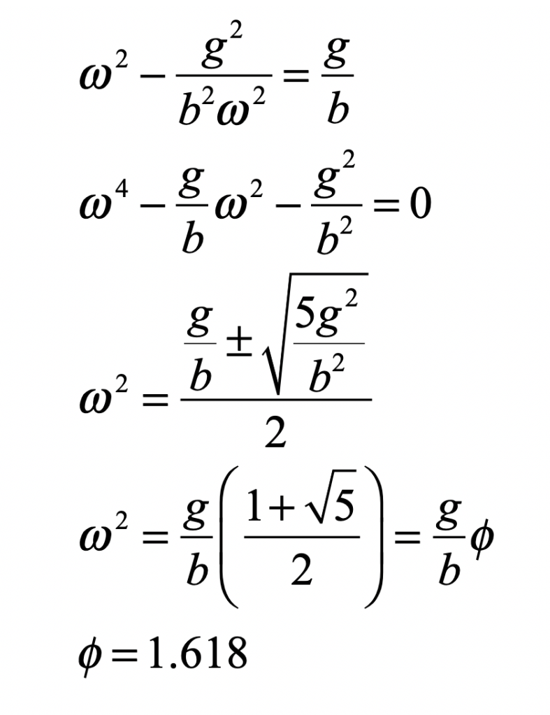
One of the key steps in the renormalization procedure was the need to identify a ratio of the sizes of smaller structures to larger structures. Feigenbaum began by studying how the bifurcations depended on the increasing growth rate. He calculated the threshold values rm for each of the bifurcations, and then took the ratios of the intervals, comparing the previous interval (rm-1 – rm-2) to the next interval (rm – rm-1). This procedure is like the well-known method to calculate the golden ratio = 1.61803 from the Fibonacci series, and Feigenbaum might have expected the golden ratio to emerge from his analysis of the logistic map. After all, the golden ratio has a scary habit of showing up in physics, just like in the KAM theory. However, as the bifurcation index m increased in Feigenbaum’s study, this ratio settled down to a limiting value of 4.66920. Then he did what anyone would do with an unfamiliar number that emerges from a physical calculation—he tried to see if it was a combination of other fundamental numbers, like pi and Euler’s constant e, and even the golden ratio. But none of these worked. He had found a new number that had universal application to chaos theory [13].

Gleick (1987)
By the mid-1980’s, chaos theory was seeping in to a broadening range of research topics that seemed to span the full breadth of science, from biology to astrophysics, from mechanics to chemistry. A particularly active group of chaos practitioners were J. Doyn Farmer, James Crutchfield, Norman Packard and Robert Shaw who founded the Dynamical Systems Collective at the University of California, Santa Cruz. One of the important outcomes of their work was a method to reconstruct the state space of a complex system using only its representative time series [14]. Their work helped proliferate the techniques of chaos theory into the mainstream. Many who started using these techniques were only vaguely aware of its long history until the science writer James Gleick wrote a best-selling history of the subject that brought chaos theory to the forefront of popular science [15]. And the rest, as they say, is history.
By David D. Nolte, April 3, 2024
References
[1] Poincaré, H. and D. L. Goroff (1993). New methods of celestial mechanics. Edited and introduced by Daniel L. Goroff. New York, American Institute of Physics.
[2] J. Barrow-Green, Poincaré and the three body problem (London Mathematical Society, 1997).
[3] Cartwright,M.L.andJ.E.Littlewood(1945).“Onthenon-lineardifferential equation of the second order. I. The equation y′′ − k(1 – yˆ2)y′ + y = bλk cos(λt + a), k large.” Journal of the London Mathematical Society 20: 180–9. Discussed in Aubin, D. and A. D. Dalmedico (2002). “Writing the History of Dynamical Systems and Chaos: Longue DurÈe and Revolution, Disciplines and Cultures.” Historia Mathematica, 29: 273.
[4] Kolmogorov, A. N., (1954). “On conservation of conditionally periodic motions for a small change in Hamilton’s function.,” Dokl. Akad. Nauk SSSR (N.S.), 98: 527–30.
[5] Lorenz, E. N. (1963). “Deterministic Nonperiodic Flow.” Journal of the Atmo- spheric Sciences 20(2): 130–41.
[6] Arnold,V.I.(1997).“From superpositions to KAM theory,”VladimirIgorevich Arnold. Selected, 60: 727–40.
[7] Moser, J. (1962). “On Invariant Curves of Area-Preserving Mappings of an Annulus.,” Nachr. Akad. Wiss. Göttingen Math.-Phys, Kl. II, 1–20.
[8] Arnold, V. I. (1963). “Small denominators and problems of the stability of motion in classical and celestial mechanics (in Russian),” Usp. Mat. Nauk., 18: 91–192,; Arnold, V. I. (1964). “Instability of Dynamical Systems with Many Degrees of Freedom.” Doklady Akademii Nauk Sssr 156(1): 9.
[9] Chirikov, B. V. (1969). Research concerning the theory of nonlinear resonance and stochasticity. Institute of Nuclear Physics, Novosibirsk. 4. Note: The Standard Map Jn+1 =Jn +εsinθn θn+1 =θn +Jn+1
is plotted in Fig. 3.31 in Nolte, Introduction to Modern Dynamics (2015) on p. 139. For small perturbation ε, two fixed points appear along the line J = 0 corresponding to p/q = 1: one is an elliptical point (with surrounding small orbits) and the other is a hyperbolic point where chaotic behavior is first observed. With increasing perturbation, q elliptical points and q hyperbolic points emerge for orbits with winding numbers p/q with small denominators (1/2, 1/3, 2/3 etc.). Other orbits with larger q are warped by the increasing perturbation but are not chaotic. These orbits reside on invariant tori, known as the KAM tori, that do not disintegrate into chaos at small perturbation. The set of KAM tori is a Cantor-like set with non- zero measure, ensuring that stable behavior can survive in the presence of perturbations, such as perturbation of the Earth’s orbit around the Sun by Jupiter. However, with increasing perturbation, orbits with successively larger values of q disintegrate into chaos. The last orbits to survive in the Standard Map are the golden mean orbits with p/q = φ–1 and p/q = 2–φ. The critical value of the perturbation required for the golden mean orbits to disintegrate into chaos is surprisingly large at εc = 0.97.
[10] Ruelle,D. and F.Takens (1971).“OntheNatureofTurbulence.”Communications in Mathematical Physics 20(3): 167–92.
[11] Gollub, J. P. and H. L. Swinney (1975). “Onset of Turbulence in a Rotating Fluid.” Physical Review Letters, 35(14): 927–30.
[12] May, R. M. (1976). “Simple Mathematical-Models with very complicated Dynamics.” Nature, 261(5560): 459–67.
[13] M. J. Feigenbaum, “Quantitative Universality for a Class of Nnon-linear Transformations,” Journal of Statistical Physics 19, 25-52 (1978).
[14] Packard, N.; Crutchfield, J. P.; Farmer, J. Doyne; Shaw, R. S. (1980). “Geometry from a Time Series”. Physical Review Letters. 45 (9): 712–716.
[15] Gleick,J.(1987).Chaos:MakingaNewScience,NewYork:Viking.p.180.