Imagine if you just discovered how to text through time, i.e. time-texting, when a close friend meets a shocking death. Wouldn’t you text yourself in the past to try to prevent it? But what if, every time you change the time-line and alter the future in untold ways, the friend continues to die, and you seemingly can never stop it? This is the premise of Stein’s Gate, a Japanese sci-fi animé bringing in the paradoxes of time travel, casting CERN as an evil clandestine spy agency, and introducing do-it-yourself inventors, hackers, and wacky characters, while it centers on a terrible death of a lovable character that can never be avoided.
It is also a good computational physics project that explores the dynamics of bifurcations, bistability and chaos. I teach a course in modern dynamics in the Physics Department at Purdue University. The topics of the course range broadly from classical mechanics to chaos theory, social networks, synchronization, nonlinear dynamics, economic dynamics, population dynamics, evolutionary dynamics, neural networks, special and general relativity, among others that are covered in the course using a textbook that takes a modern view of dynamics [1].
For the final project of the second semester the students (Junior physics majors) are asked to combine two or three of the topics into a single project. Students have come up with a lot of creative combinations: population dynamics of zombies, nonlinear dynamics of negative gravitational mass, percolation of misinformation in presidential elections, evolutionary dynamics of neural architecture, and many more. In that spirit, and for a little fun, in this blog I explore the so-called physics of Stein’s Gate.
Stein’s Gate and the Divergence Meter
Stein’s Gate is a Japanese TV animé series that had a world-wide distribution in 2011. The central premise of the plot is that certain events always occur even if you are on different timelines—like trying to avoid someone’s death in an accident.
This is the problem confronting Rintaro Okabe who tries to stop an accident that kills his friend Mayuri Shiina. But every time he tries to change time, she dies in some other way. It turns out that all the nearby timelines involve her death. According to a device known as The Divergence Meter, Rintaro must get farther than 4% away from the original timeline to have a chance to avoid the otherwise unavoidable event.
This is new. Usually, time-travel Sci-Fi is based on the Butterfly Effect. Chaos theory is characterized by something called sensitivity to initial conditions (SIC), meaning that slightly different starting points produce trajectories that diverge exponentially from nearby trajectories. It is called the Butterfly Effect because of the whimsical notion that a butterfly flapping its wings in China can cause a hurricane in Florida. In the context of the butterfly effect, if you go back in time and change anything at all, the effect cascades through time until the present time in unrecognizable. As an example, in one episode of the TV cartoon The Simpsons, Homer goes back in time to the age of the dinosaurs and kills a single mosquito. When he gets back to our time, everything has changed in bazaar and funny ways.
Stein’s Gate introduces a creative counter example to the Butterfly Effect. Instead of scrambling the future when you fiddle with the past, you find that you always get the same event, even when you change a lot of the conditions—Mayuri still dies. This sounds eerily familiar to a physicist who knows something about chaos theory. It means that the unavoidable event is acting like a stable fixed point in the time dynamics—an attractor! Even if you change the initial conditions, the dynamics draw you back to the fixed point—in this case Mayuri’s accident. What would this look like in a dynamical system?
The Local Basin of Attraction
Dynamical systems can be described as trajectories in a high-dimensional state space. Within state space there are special points where the dynamics are static—known as fixed points. For a stable fixed point, a slight perturbation away will relax back to the fixed point. For an unstable fixed point, on the other hand, a slight perturbation grows and the system dynamics evolve away. However, there can be regions in state space where every initial condition leads to trajectories that stay within that region. This is known as a basin of attraction, and the boundaries of these basins are called separatrixes.
A high-dimensional state space can have many basins of attraction. All the physics that starts within a basin stays within that basin—almost like its own self-consistent universe, bordered by countless other universes. There are well-known physical systems that have many basins of attraction. String theory is suspected to generate many adjacent universes where the physical laws are a little different in each basin of attraction. Spin glasses, which are amorphous solid-state magnets, have this property, as do recurrent neural networks like the Hopfield network. Basins of attraction occur naturally within the physics of these systems.
It is possible to embed basins of attraction within an existing dynamical system. As an example, let’s start with one of the simplest types of dynamics, a hyperbolic fixed point
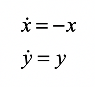
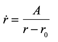
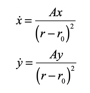
that has a single saddle fixed point at the origin. We want to add a basin of attraction at the origin with a domain range given by a radius r0. At the same time, we want to create a separatrix that keeps the outer hyperbolic dynamics separate from the internal basin dynamics. To keep all outer trajectories in the outer domain, we can build a dynamical barrier to prevent the trajectories from crossing the separatrix. This can be accomplished by adding a radial repulsive term
In x-y coordinates this is
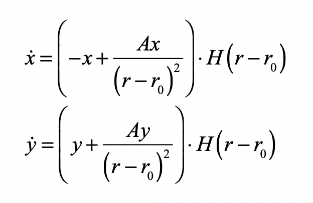
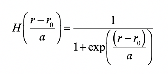
We also want to keep the internal dynamics of our basin separate from the external dynamics. To do this, we can multiply by a sigmoid function, like a Heaviside function H(r-r0), to zero-out the external dynamics inside our basin. The final external dynamics is then
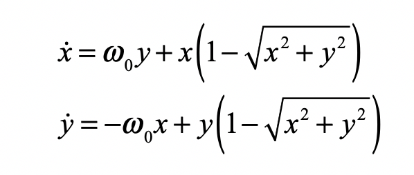
Now we have to add the internal dynamics for the basin of attraction. To make it a little more interesting, let’s make the internal dynamics an autonomous oscillator
Putting this all together, gives
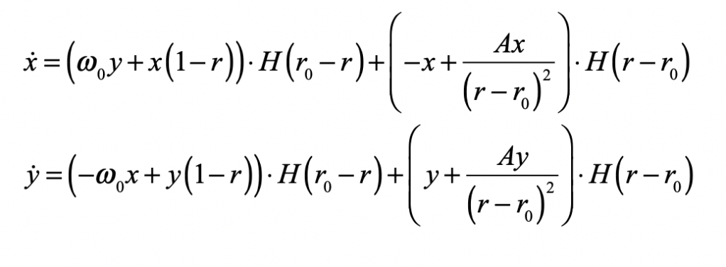
This looks a little complex, for such a simple model, but it illustrates the principle. The sigmoid is best if it is differentiable, so instead of a Heaviside function it can be a Fermi function
The phase-space portrait of the final dynamics looks like
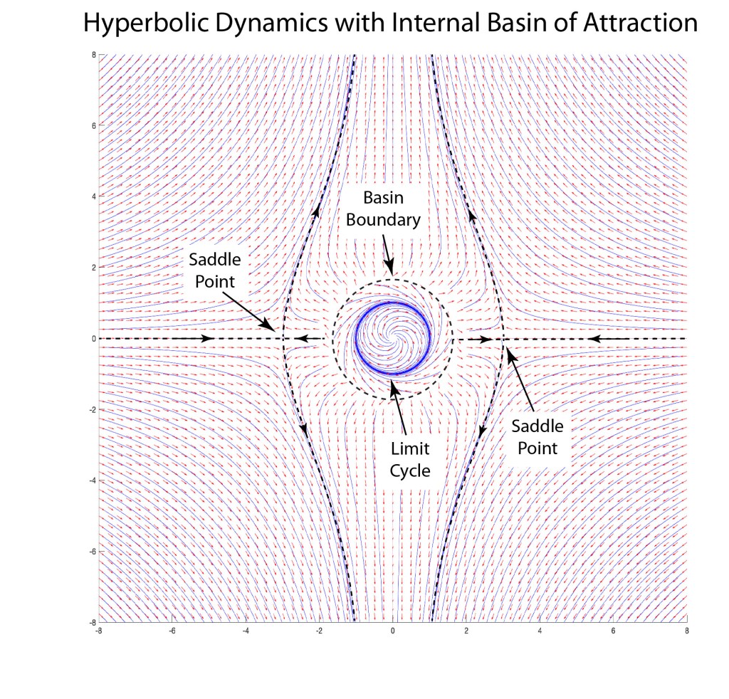
Adding the internal dynamics does not change the far-field external dynamics, which are still hyperbolic. The repulsive term does split the central saddle point into two saddle points, one on each side left-and-right, so the repulsive term actually splits the dynamics. But the internal dynamics are self-contained and separate from the external dynamics. The origin is an unstable spiral that evolves to a limit cycle. The basin boundary has marginal stability and is known as a “wall”.
To verify the stability of the external fixed point, find the fixed point coordinates
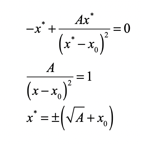
and evaluate the Jacobian matrix (for A = 1 and x0 = 2)
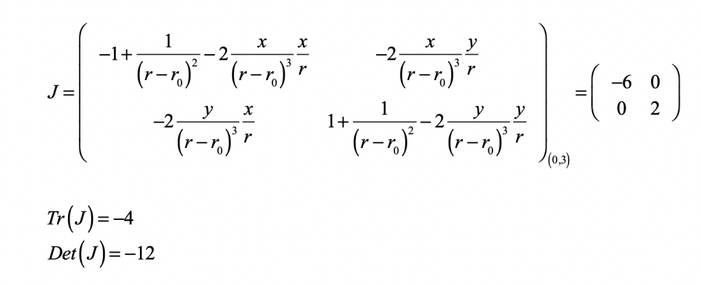
which is clearly a saddle point because the determinant is negative.
In the context of Stein’s Gate, the basin boundary is equivalent to the 4% divergence which is necessary to escape the internal basin of attraction where Mayuri meets her fate.
Python Program: SteinsGate2D.py
#!/usr/bin/env python3
# -*- coding: utf-8 -*-
"""
SteinsGate2D.py
Created on Sat March 6, 2021

@author: David Nolte
Introduction to Modern Dynamics, 2nd edition (Oxford University Press, 2019)

2D simulation of Stein's Gate Divergence Meter
"""
import numpy as np
from scipy import integrate
from matplotlib import pyplot as plt

plt.close('all')

def solve_flow(param,lim = [-6,6,-6,6],max_time=20.0):

    def flow_deriv(x_y, t0, alpha, beta, gamma):
        #"""Compute the time-derivative ."""
        x, y = x_y

        w = 1
        R2 = x**2 + y**2
        R = np.sqrt(R2)
        arg = (R-2)/0.1
        env1 = 1/(1+np.exp(arg))
        env2 = 1 - env1

        f = env2*(x*(1/(R-1.99)**2 + 1e-2) - x) + env1*(w*y + w*x*(1 - R))
        g = env2*(y*(1/(R-1.99)**2 + 1e-2) + y) + env1*(-w*x + w*y*(1 - R))

        return [f,g]
    model_title = 'Steins Gate'

    plt.figure()
    xmin = lim[0]
    xmax = lim[1]
    ymin = lim[2]
    ymax = lim[3]
    plt.axis([xmin, xmax, ymin, ymax])

    N = 24*4 + 47
    x0 = np.zeros(shape=(N,2))
    ind = -1
    for i in range(0,24):
        ind = ind + 1
        x0[ind,0] = xmin + (xmax-xmin)*i/23
        x0[ind,1] = ymin
        ind = ind + 1
        x0[ind,0] = xmin + (xmax-xmin)*i/23
        x0[ind,1] = ymax
        ind = ind + 1
        x0[ind,0] = xmin
        x0[ind,1] = ymin + (ymax-ymin)*i/23
        ind = ind + 1
        x0[ind,0] = xmax
        x0[ind,1] = ymin + (ymax-ymin)*i/23
    ind = ind + 1
    x0[ind,0] = 0.05
    x0[ind,1] = 0.05

    for thetloop in range(0,10):
        ind = ind + 1
        theta = 2*np.pi*(thetloop)/10
        ys = 0.125*np.sin(theta)
        xs = 0.125*np.cos(theta)
        x0[ind,0] = xs
        x0[ind,1] = ys

    for thetloop in range(0,10):
        ind = ind + 1
        theta = 2*np.pi*(thetloop)/10
        ys = 1.7*np.sin(theta)
        xs = 1.7*np.cos(theta)
        x0[ind,0] = xs
        x0[ind,1] = ys

    for thetloop in range(0,20):
        ind = ind + 1
        theta = 2*np.pi*(thetloop)/20
        ys = 2*np.sin(theta)
        xs = 2*np.cos(theta)
        x0[ind,0] = xs
        x0[ind,1] = ys

    ind = ind + 1
    x0[ind,0] = -3
    x0[ind,1] = 0.05
    ind = ind + 1
    x0[ind,0] = -3
    x0[ind,1] = -0.05
    ind = ind + 1
    x0[ind,0] = 3
    x0[ind,1] = 0.05
    ind = ind + 1
    x0[ind,0] = 3
    x0[ind,1] = -0.05
    ind = ind + 1
    x0[ind,0] = -6
    x0[ind,1] = 0.00
    ind = ind + 1
    x0[ind,0] = 6
    x0[ind,1] = 0.00

    colors = plt.cm.prism(np.linspace(0, 1, N))

    # Solve for the trajectories
    t = np.linspace(0, max_time, int(250*max_time))
    x_t = np.asarray([integrate.odeint(flow_deriv, x0i, t, param)
                      for x0i in x0])

    for i in range(N):
        x, y = x_t[i,:,:].T
        lines = plt.plot(x, y, '-', c=colors[i])
        plt.setp(lines, linewidth=1)

    plt.show()
    plt.title(model_title)

    return t, x_t

param = (0.02,0.5,0.2)        # Steins Gate
lim = (-6,6,-6,6)

t, x_t = solve_flow(param,lim)

plt.savefig('Steins Gate')
The Lorenz Butterfly
Two-dimensional phase space cannot support chaos, and we would like to reconnect the central theme of Stein’s Gate, the Divergence Meter, with the Butterfly Effect. Therefore, let’s actually incorporate our basin of attraction inside the classic Lorenz Butterfly. The goal is to put an attracting domain into the midst of the three-dimensional state space of the Lorenz butterfly in a way that repels the butterfly, without destroying it, but attracts local trajectories. The question is whether the butterfly can survive if part of its state space is made unavailable to it.
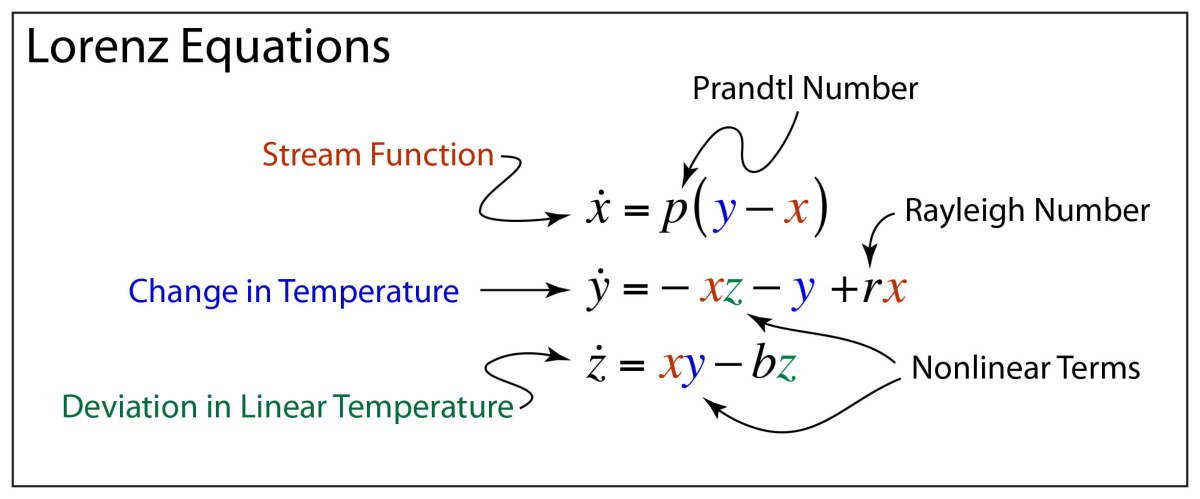
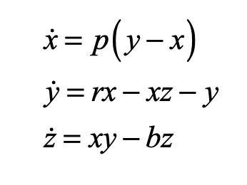
The classic Lorenz dynamical system is
As in the 2D case, we will put in a repelling barrier that prevents external trajectories from moving into the local basin, and we will isolate the external dynamics by using the sigmoid function. The final flow equations looks like
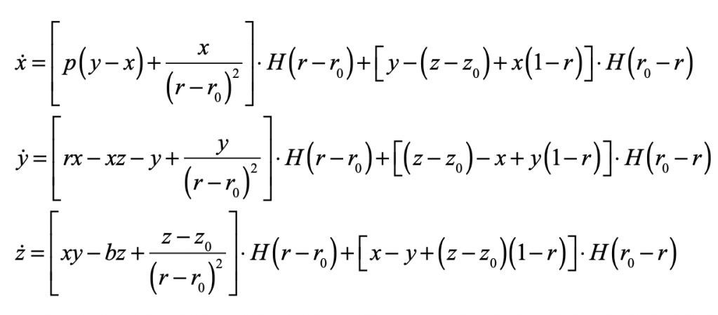
where the radius is relative to the center of the attracting basin
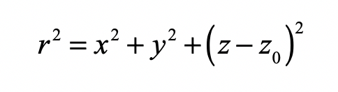
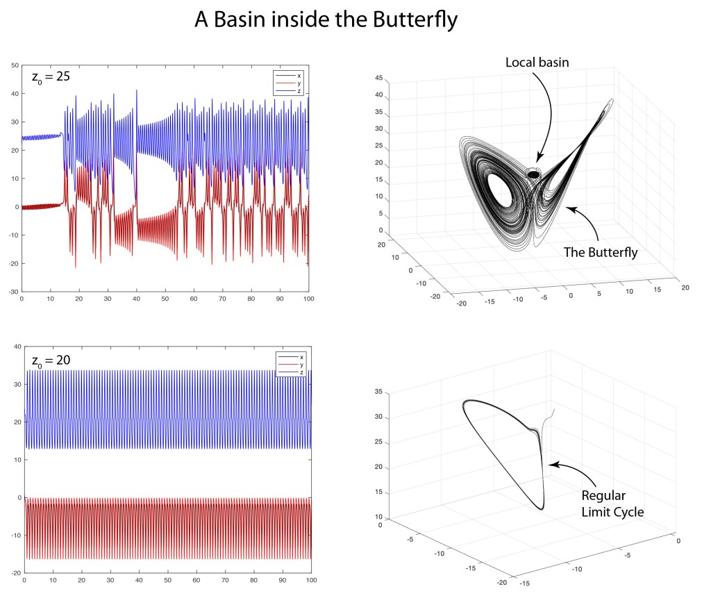
and r0 is the radius of the basin. The center of the basin is at [x0, y0, z0] and we are assuming that x0 = 0 and y0 = 0 and z0 = 25 for the standard Butterfly parameters p = 10, r = 25 and b = 8/3. This puts our basin of attraction a little on the high side of the center of the Butterfly. If we embed it too far inside the Butterfly it does actually destroy the Butterfly dynamics.
When r0 = 0, the dynamics of the Lorenz’ Butterfly are essentially unchanged. However, when r0 = 1.5, then there is a repulsive effect on trajectories that pass close to the basin. It can be seen as part of the trajectory skips around the outside of the basin in Figure 2.
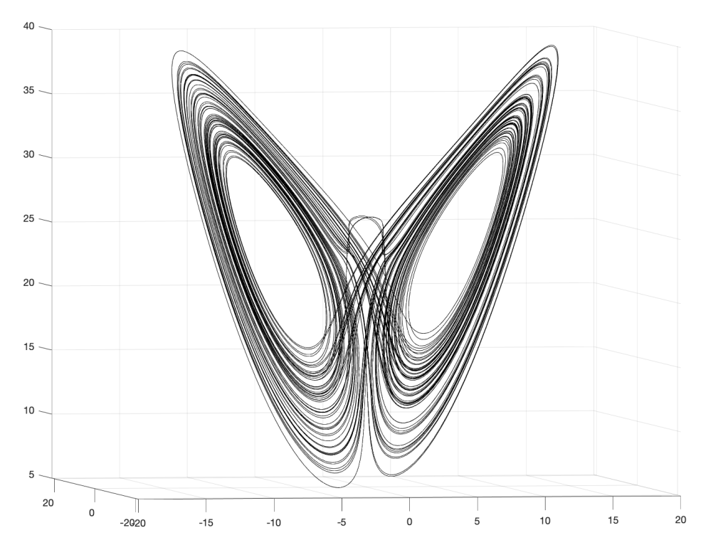
Trajectories can begin very close to the basin, but still on the outside of the separatrix, as in the top row of Figure 3 where the basin of attraction with r0 = 1.5 lies a bit above the center of the Butterfly. The Butterfly still exists for the external dynamics. However, any trajectory that starts within the basin of attraction remains there and executes a stable limit cycle. This is the world where Mayuri dies inside the 4% divergence. But if the initial condition can exceed 4%, then the Butterfly effect takes over. The bottom row of Figure 2 shows that the Butterfly itself is fragile. When the external dynamics are perturbed more strongly by more closely centering the local basin, the hyperbolic dynamics of the Butterfly are impeded and the external dynamics are converted to a stable limit cycle. It is interesting that the Butterfly, so often used as an illustration of sensitivity to initial conditions (SIC), is itself sensitive to perturbations that can convert it away from chaos and back to regular motion.
Discussion and Extensions
In the examples shown here, the local basin of attraction was put in “by hand” as an isolated region inside the dynamics. It would be interesting to consider more natural systems, like a spin glass or a Hopfield network, where the basins of attraction occur naturally from the physical principles of the system. Then we could use the “Divergence Meter” to explore these physical systems to see how far the dynamics can diverge before crossing a separatrix. These systems are impossible to visualize because they are intrinsically very high dimensional systems, but Monte Carlo approaches could be used to probe the “sizes” of the basins.
Another interesting extension would be to embed these complex dynamics into spacetime. Since this all started with the idea of texting through time, it would be interesting (and challenging) to see how we could describe this process in a high dimensional Minkowski space that had many space dimensions (but still only one time dimension). Certainly it would violate the speed of light criterion, but we could then take the approach of David Deutsch and view the time axis as if it had multiple branches, like the branches of the arctangent function, creating time-consistent sheets within a sheave of flat Minkowski spaces.
References
[1] D. D. Nolte, Introduction to Modern Dynamics: Chaos, Networks, Space and Time, 2nd edition (Oxford University Press, 2019)
[2] E. N. Lorenz, The essence of chaos. (University of Washington Press, 1993)
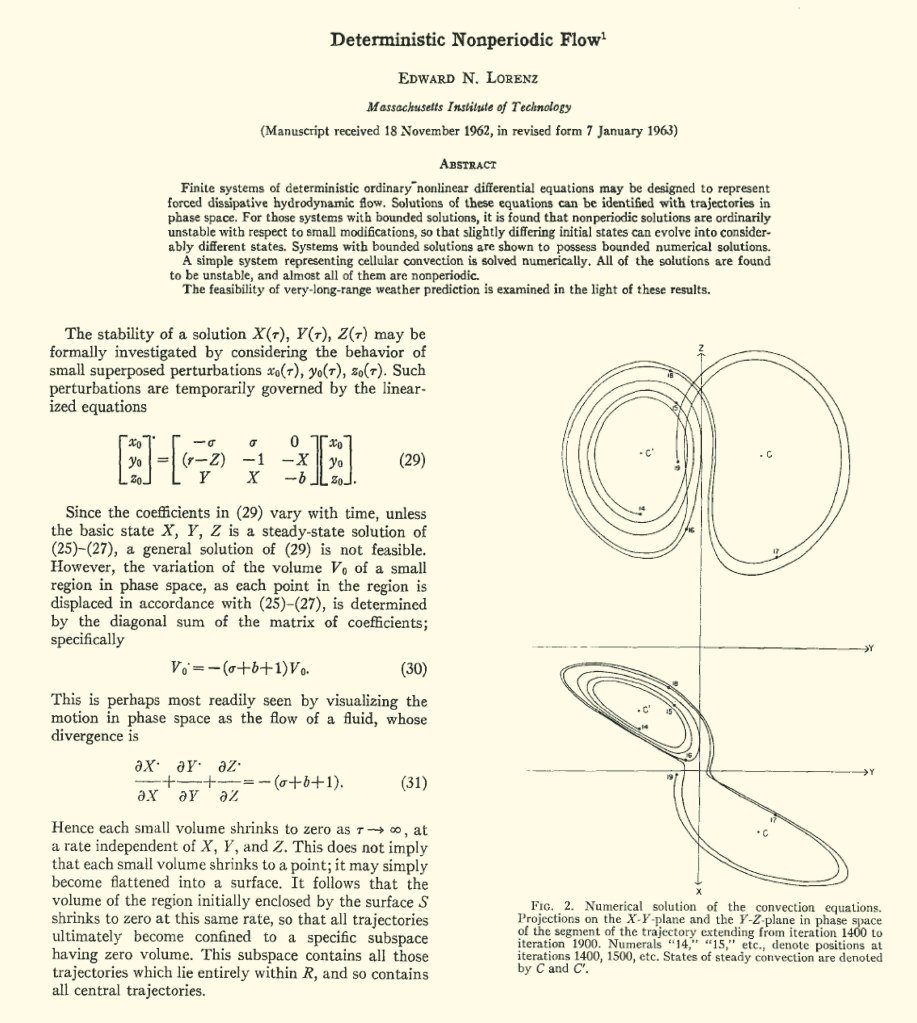
[3] E. N. Lorenz, “Deterministic Nonperiodic Flow,” Journal of the Atmospheric Sciences, vol. 20, no. 2, pp. 130-141, 1963 (1963)
This Blog Post is a Companion to the undergraduate physics textbook Modern Dynamics: Chaos, Networks, Space and Time, 2nd ed. (Oxford, 2019) introducing Lagrangians and Hamiltonians, chaos theory, complex systems, synchronization, neural networks, econophysics and Special and General Relativity.