
The butterfly effect is one of the most widely known principles of chaos theory. It has become a meme, propagating through popular culture in movies, books, TV shows and even casual conversation.
Can a butterfly flapping its wings in Florida send a hurricane to New York?
The origin of the butterfly effect is — not surprisingly — the image of a butterfly-like set of trajectories that was generated, in one of the first computer simulations of chaos theory, by Edward Lorenz.
Lorenz’ Butterfly
Excerpted from Galileo Unbound (Oxford, 2018) pg. 215
When Edward Lorenz (1917 – 2008) was a child, he memorized all perfect squares up to ten thousand. This obvious interest in mathematics led him to a master’s degree in the subject at Harvard in 1940 under the supervision of Georg Birkhoff. Lorenz’s master’s thesis was on an aspect of Riemannian geometry, but his foray into nonlinear dynamics was triggered by the intervention of World War II. Only a few months before receiving his doctorate in mathematics from Harvard, the Japanese bombed Pearl Harbor.
Lorenz left the PhD program at Harvard to join the United States Army Air Force to train as a weather forecaster in early 1942, and he took courses on forecasting and meteorology at MIT. After receiving a second master’s degree, this time in meteorology, Lorenz was posted to Hawaii, then to Saipan and finally to Guam. His area of expertise was in high-level winds, which were important for high-altitude bombing missions during the final months of the war in the Pacific. After the Japanese surrender, Lorenz returned to MIT, where he continued his studies in meteorology, receiving his doctorate degree in 1948 with a thesis on the application of fluid dynamical equations to predict the motion of storms.
One of Lorenz’ colleagues at MIT was Norbert Wiener (1894 – 1964), with whom he sometimes played chess during lunch at the faculty club. Wiener had published his landmark book Cybernetics: Control and Communication in the Animal and Machine in 1949 which arose out of the apparently mundane problem of gunnery control during the Second World War. As an abstract mathematician, Wiener attempted to apply his cybernetic theory to the complexities of weather, but he developed a theorem concerning nonlinear fluid dynamics which appeared to show that linear interpolation, of sufficient resolution, would suffice for weather forecasting, possibly even long-range forecasting. Many on the meteorology faculty embraced this theorem because it fell in line with common practices of the day in which tomorrow’s weather was predicted using linear regression on measurements taken today. However, Lorenz was skeptical, having acquired a detailed understanding of atmospheric energy cascades as larger vortices induced smaller vortices all the way down to the molecular level, dissipating as heat, and then all the way back up again as heat drove large-scale convection. This was clearly not a system that would yield to linearization. Therefore, Lorenz determined to solve nonlinear fluid dynamics models to test this conjecture.
Even with a computer in hand, the atmospheric equations needed to be simplified to make the calculations tractable. Lorenz was more a scientist than an engineer, and more of a meteorologist than a forecaster. He did not hesitate to make simplifying assumptions if they retained the correct phenomenological behavior, even if they no longer allowed for accurate weather predictions.
He had simplified the number of atmospheric equations down to twelve. Progress was good, and by 1961, he had completed a large initial numerical study. He focused on nonperiodic solutions, which he suspected would deviate significantly from the predictions made by linear regression, and this hunch was vindicated by his numerical output. One day, as he was testing his results, he decided to save time by starting the computations midway by using mid-point results from a previous run as initial conditions. He typed in the three-digit numbers from a paper printout and went down the hall for a cup of coffee. When he returned, he looked at the printout of the twelve variables and was disappointed to find that they were not related to the previous full-time run. He immediately suspected a faulty vacuum tube, as often happened. But as he looked closer at the numbers, he realized that, at first, they tracked very well with the original run, but then began to diverge more and more rapidly until they lost all connection with the first-run numbers. His initial conditions were correct to a part in a thousand, but this small error was magnified exponentially as the solution progressed.
At this point, Lorenz recalled that he “became rather excited”. He was looking at a complete breakdown of predictability in atmospheric science. If radically different behavior arose from the smallest errors, then no measurements would ever be accurate enough to be useful for long-range forecasting. At a more fundamental level, this was a break with a long-standing tradition in science and engineering that clung to the belief that small differences produced small effects. What Lorenz had discovered, instead, was that the deterministic solution to his 12 equations was exponentially sensitive to initial conditions (known today as SIC).
The Lorenz Equations
Over the following months, he was able to show that SIC was a result of the nonperiodic solutions. The more Lorenz became familiar with the behavior of his equations, the more he felt that the 12-dimensional trajectories had a repeatable shape. He tried to visualize this shape, to get a sense of its character, but it is difficult to visualize things in twelve dimensions, and progress was slow. Then Lorenz found that when the solution was nonperiodic (the necessary condition for SIC), four of the variables settled down to zero, leaving all the dynamics to the remaining three variables.
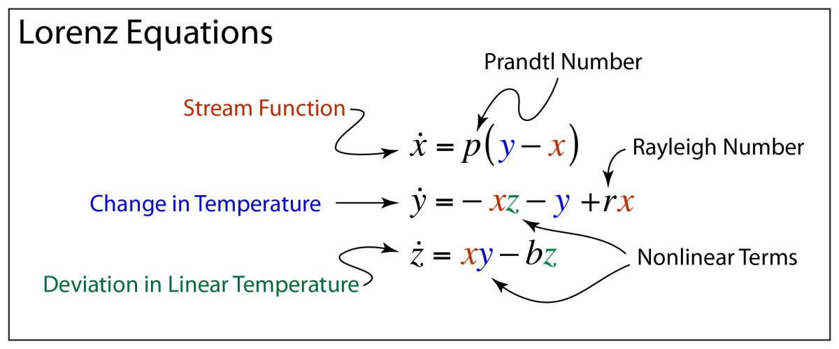
Lorenz narrowed the equations of atmospheric instability down to three variables: the stream function, the change in temperature and the deviation in linear temperature. The only parameter in the stream function is something known as the Prandtl Number. This is a dimensionless number which is the ratio of the kinetic viscosity of the fluid to its thermal diffusion coefficient and is a physical property of the fluid. The only parameter in the change in temperature is the Rayleigh Number which is a dimensionless parameter proportional to the difference in temperature between the top and the bottom of the fluid layer. The final parameter, in the equation for the deviation in linear temperature, is the ratio of the height of the fluid layer to the width of the convection rolls. The final simplified model is given by the flow equations

The Butterfly
Lorenz finally had a 3-variable dynamical system that displayed chaos. Moreover, it had a three-dimensional state space that could be visualized directly. He ran his simulations, exploring the shape of the trajectories in three-dimensional state space for a wide range of initial conditions, and the trajectories did indeed always settle down to restricted regions of state space. They relaxed in all cases to a sort of surface that was elegantly warped, with wing-like patterns like a butterfly, as the state point of the system followed its dynamics through time. The attractor of the Lorenz equations was strange. Later, in 1971, David Ruelle (1935 – ), a Belgian-French mathematical physicist named this a “strange attractor”, and this name has become a standard part of the language of the theory of chaos.
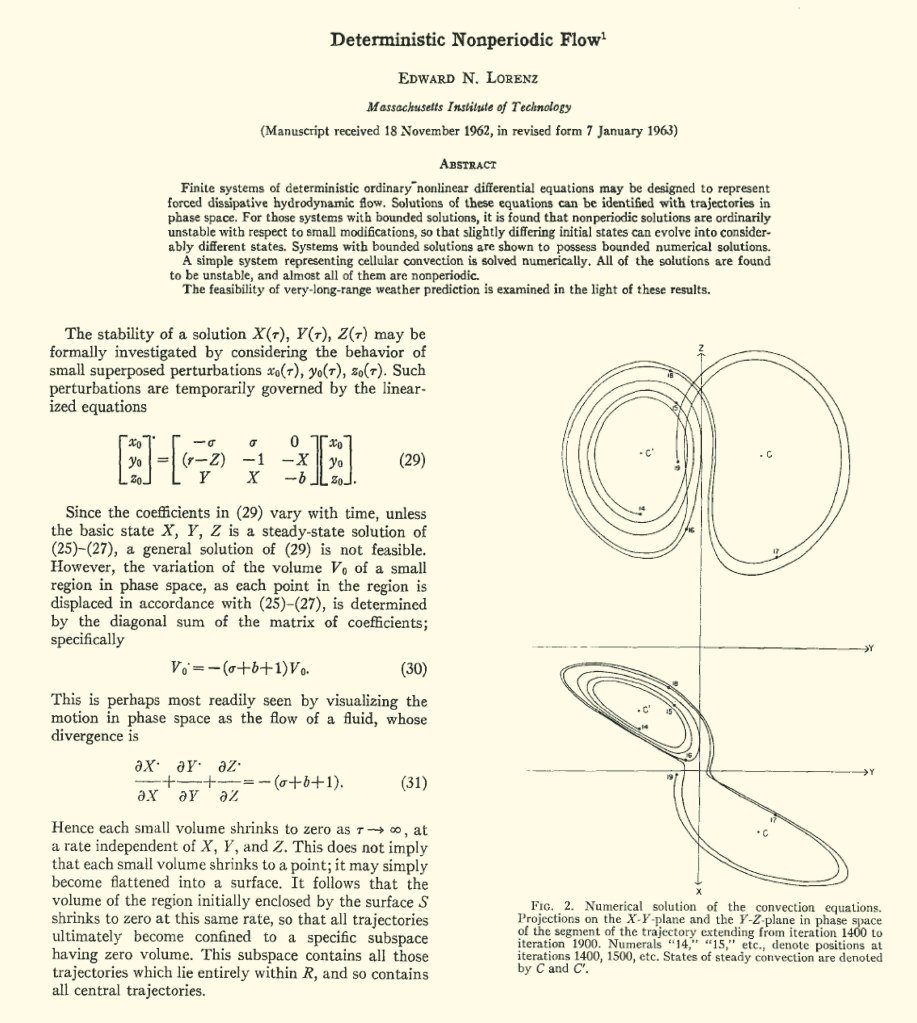
The first graphical representation of the butterfly attractor is shown in Fig. 1 drawn by Lorenz for his 1963 publication.
Using our modern plotting ability, the 3D character of the butterfly is shown in Fig. 2

A projection onto the x-y plane is shown in Fig. 3. In the full 3D state space the trajectories never overlap, but in the projection onto a 2D plane the trajectories are moving above and below each other.

The reason it is called a strange attractor is because all initial conditions relax onto the strange attractor, yet every trajectory on the strange attractor separates exponentially from neighboring trajectories, displaying the classic SIC property of chaos. So here is an elegant collection of trajectories that are certainly not just random noise, yet detailed prediction is still impossible. Deterministic chaos has significant structure, and generates beautiful patterns, without actual “randomness”.
Python Program
#!/usr/bin/env python3
# -*- coding: utf-8 -*-
"""
Created on Mon Apr 16 07:38:57 2018

@author: nolte
Introduction to Modern Dynamics, 2nd edition (Oxford University Press, 2019)

Lorenz model of atmospheric turbulence
"""
import numpy as np
import matplotlib as mpl

import matplotlib.colors as colors
import matplotlib.cm as cmx

from scipy import integrate
from matplotlib import cm
from matplotlib import pyplot as plt
from mpl_toolkits.mplot3d import Axes3D
from matplotlib.colors import cnames
from matplotlib import animation

plt.close('all')

jet = cm = plt.get_cmap('jet')
values = range(10)
cNorm  = colors.Normalize(vmin=0, vmax=values[-1])
scalarMap = cmx.ScalarMappable(norm=cNorm, cmap=jet)

def solve_lorenz(N=12, angle=0.0, max_time=8.0, sigma=10.0, beta=8./3, rho=28.0):

    fig = plt.figure()
    ax = fig.add_axes([0, 0, 1, 1], projection='3d')
    ax.axis('off')

    # prepare the axes limits
    ax.set_xlim((-25, 25))
    ax.set_ylim((-35, 35))
    ax.set_zlim((5, 55))

    def lorenz_deriv(x_y_z, t0, sigma=sigma, beta=beta, rho=rho):
        """Compute the time-derivative of a Lorenz system."""
        x, y, z = x_y_z
        return [sigma * (y - x), x * (rho - z) - y, x * y - beta * z]

    # Choose random starting points, uniformly distributed from -15 to 15
    np.random.seed(1)
    x0 = -10 + 20 * np.random.random((N, 3))

    # Solve for the trajectories
    t = np.linspace(0, max_time, int(500*max_time))
    x_t = np.asarray([integrate.odeint(lorenz_deriv, x0i, t)
                      for x0i in x0])

    # choose a different color for each trajectory
    # colors = plt.cm.viridis(np.linspace(0, 1, N))
    # colors = plt.cm.rainbow(np.linspace(0, 1, N))
    # colors = plt.cm.spectral(np.linspace(0, 1, N))
    colors = plt.cm.prism(np.linspace(0, 1, N))

    for i in range(N):
        x, y, z = x_t[i,:,:].T
        lines = ax.plot(x, y, z, '-', c=colors[i])
        plt.setp(lines, linewidth=1)

    ax.view_init(30, angle)
    plt.show()

    return t, x_t


t, x_t = solve_lorenz(angle=0, N=12)

plt.figure(2)
lines = plt.plot(t,x_t[1,:,0],t,x_t[1,:,1],t,x_t[1,:,2])
plt.setp(lines, linewidth=1)
lines = plt.plot(t,x_t[2,:,0],t,x_t[2,:,1],t,x_t[2,:,2])
plt.setp(lines, linewidth=1)
lines = plt.plot(t,x_t[10,:,0],t,x_t[10,:,1],t,x_t[10,:,2])
plt.setp(lines, linewidth=1)
To explore the parameter space of the Lorenz attractor, the key parameters to change are sigma (the Prandtl number), r (the Rayleigh number) and b on line 31 of the Python code.
References
[1] E. N. Lorenz, The essence of chaos (The Jessie and John Danz lectures; Jessie and John Danz lectures.). Seattle :: University of Washington Press (in English), 1993.
[2] E. N. Lorenz, “Deterministic Nonperiodic Flow,” Journal of the Atmospheric Sciences, vol. 20, no. 2, pp. 130-141, 1963 (1963)


