Biased Double-well Potential: Bistability, Bifurcation and Hysteresis

Bistability, bifurcation and hysteresis are ubiquitous phenomena that arise from nonlinear dynamics and have considerable importance for technology applications.  For instance, the hysteresis associated with the flipping of magnetic domains under magnetic fields is the central mechanism for magnetic memory, and bistability is a key feature of switching technology.

… one of the most commonly encountered bifurcations is called a saddle-node bifurcation, which is the bifurcation that occurs in the biased double-well potential.

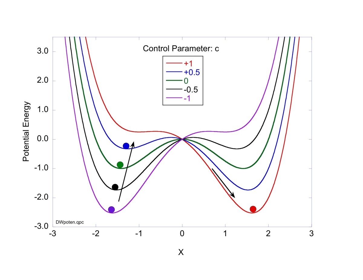
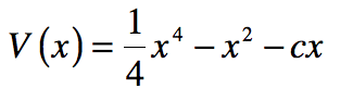
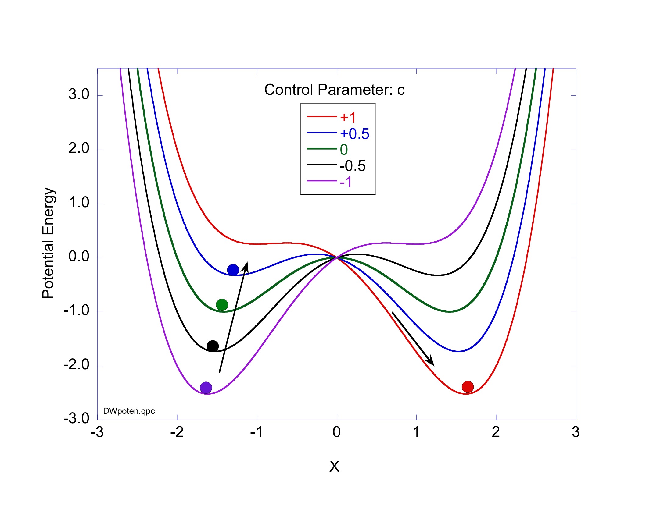
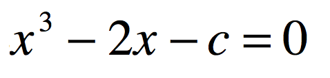
One of the simplest models for bistability and hysteresis is the one-dimensional double-well potential biased by a changing linear potential.  An example of a double-well potential with a bias is

where the parameter c is a control parameter (bias) that can be adjusted or that changes slowly in time c(t).  This dynamical system is also known as the Duffing oscillator. The net double-well potentials for several values of the control parameter c are shown in Fig. 1.   With no bias, there are two degenerate energy minima.  As c is made negative, the left well has the lowest energy, and as c is made positive the right well has the lowest energy.

The dynamics of this potential energy profile can be understood by imagining a small ball that responds to the local forces exerted by the potential.  For large negative values of c the ball will have its minimum energy in the left well.  As c is increased, the energy of the left well increases, and rises above the energy of the right well.  If the ball began in the left well, even when the left well has a higher energy than the right, there is a potential barrier that the ball cannot overcome and it remains on the left.  This local minimum is a stable equilibrium, but it is called “metastable” because it is not a global minimum of the system.  Metastability is the origin of hysteresis.

Fig. 1 A biased double-well potential in one dimension. The thresholds to destroy the local metastable minima are c = +/-1.05. For values beyond threshold, only a single minimum exists with no barrier. Hysteresis is caused by the mass being stuck in the metastable (upper) minimum because it has insufficient energy to overcome the potential barrier, until the barrier disappears at threshold and the ball rolls all the way down to the bottom to the new location. When the bias is slowly reversed, the new location becomes metastable, until the ball can overcome the barrier and roll down to its original minimum, etc.

           Once sufficient bias is applied that the local minimum disappears, the ball will roll downhill to the new minimum on the right, and in the presence of dissipation, it will come to rest in the new minimum.  The bias can then be slowly lowered, reversing this process. Because of the potential barrier, the bias must change sign and be strong enough to remove the stability of the now metastable fixed point with the ball on the right, allowing the ball to roll back down to its original location on the left.  This “overshoot” defines the extent of the hysteresis. The fact that there are two minima, and that one is metastable with a barrier between the two, produces “bistability”, meaning that there are two stable fixed points for the same control parameter.

           For illustration, assume a mass obeys the flow equation

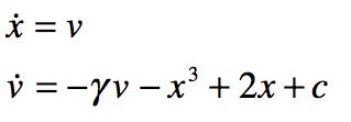
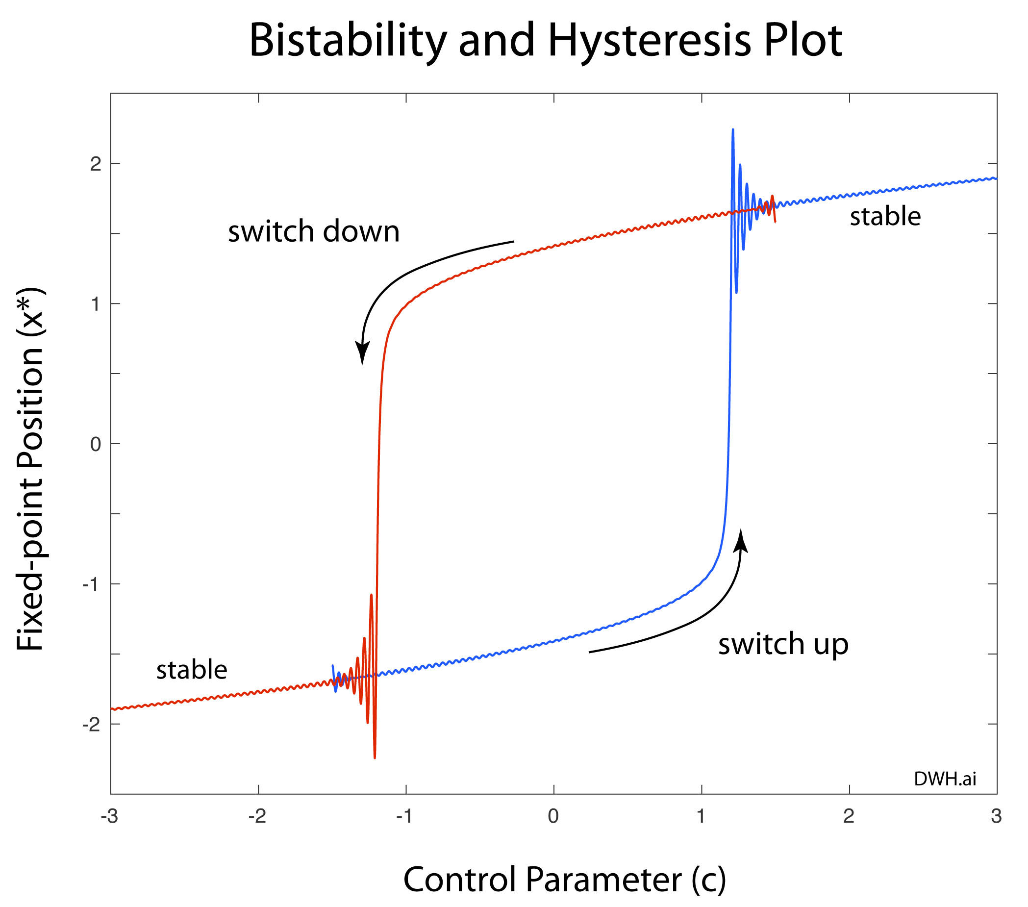
including a damping term, where the force is the negative gradient of the potential energy.  The bias parameter c can be time dependent, beginning beyond the negative threshold and slowly increasing until it exceeds the positive threshold, and then reversing and decreasing again.  The position of the mass is locally a damped oscillator until a threshold is passed, and then the mass falls into the global minimum, as shown in Fig. 2. As the bias is reversed, it remains in the metastable minimum on the right until the control parameter passes threshold, and then the mass drops into the left minimum that is now a global minimum.

Fig. 2 Hysteresis diagram. The mass begins in the left well. As the parameter c increases, the mass remains in the well, even though it is no longer the global minimum when c becomes positive. When c passes the positive threshold (around 1.05 for this example), the mass falls into the right well, with damped oscillation. Then the control parameter c is decreased slowly until the negative threshold is passed, and the mass switches to the left well with damped oscillations. The difference between the “switch up” and “switch down” values of the control parameter represents the “hysteresis” of the this system.

The sudden switching of the biased double-well potential represents what is known as a “bifurcation”. A bifurcation is a sudden change in the qualitative behavior of a system caused by a small change in a control variable. Usually, a bifurcation occurs when the number of attractors of a system changes. There is a fairly large menagerie of different types of bifurcations, but one of the most commonly encountered bifurcations is called a saddle-node bifurcation, which is the bifurcation that occurs in the biased double-well potential. In fact, there are two saddle-node bifurcations.

Bifurcations are easily portrayed by creating a joint space between phase space and the one (or more) control parameters that induce the bifurcation. The phase space of the double well is two dimensional (position, velocity) with three fixed points, but the change in the number of fixed points can be captured by taking a projection of the phase space onto a lower-dimensional manifold. In this case, the projection is simply along the x-axis. Therefore a “co-dimensional phase space” can be constructed with the x-axis as one dimension and the control parameter as the other. This is illustrated in Fig. 3. The cubic curve traces out the solutions to the fixed-point equation

For a given value of the control parameter c there are either three solutions or one solution. The values of c where the number of solutions changes discontinuously is the bifurcation point c*. Two examples of the potential function are shown on the right for c = +1 and c = -0.5 showing the locations of the three fixed points.

Fig. 3 The co-dimension phase space combines the one-dimensional dynamics along the position x with the control parameter. For a given value of c, there are three or one solution for the fixed point. When there are three solutions, two are stable (the double minima) and one is unstable (the saddle). As the magnitude of the bias increases, one stable node annihilates with the unstable node (a minimum and the saddle merge) and the dynamics “switch” to the other minimum.

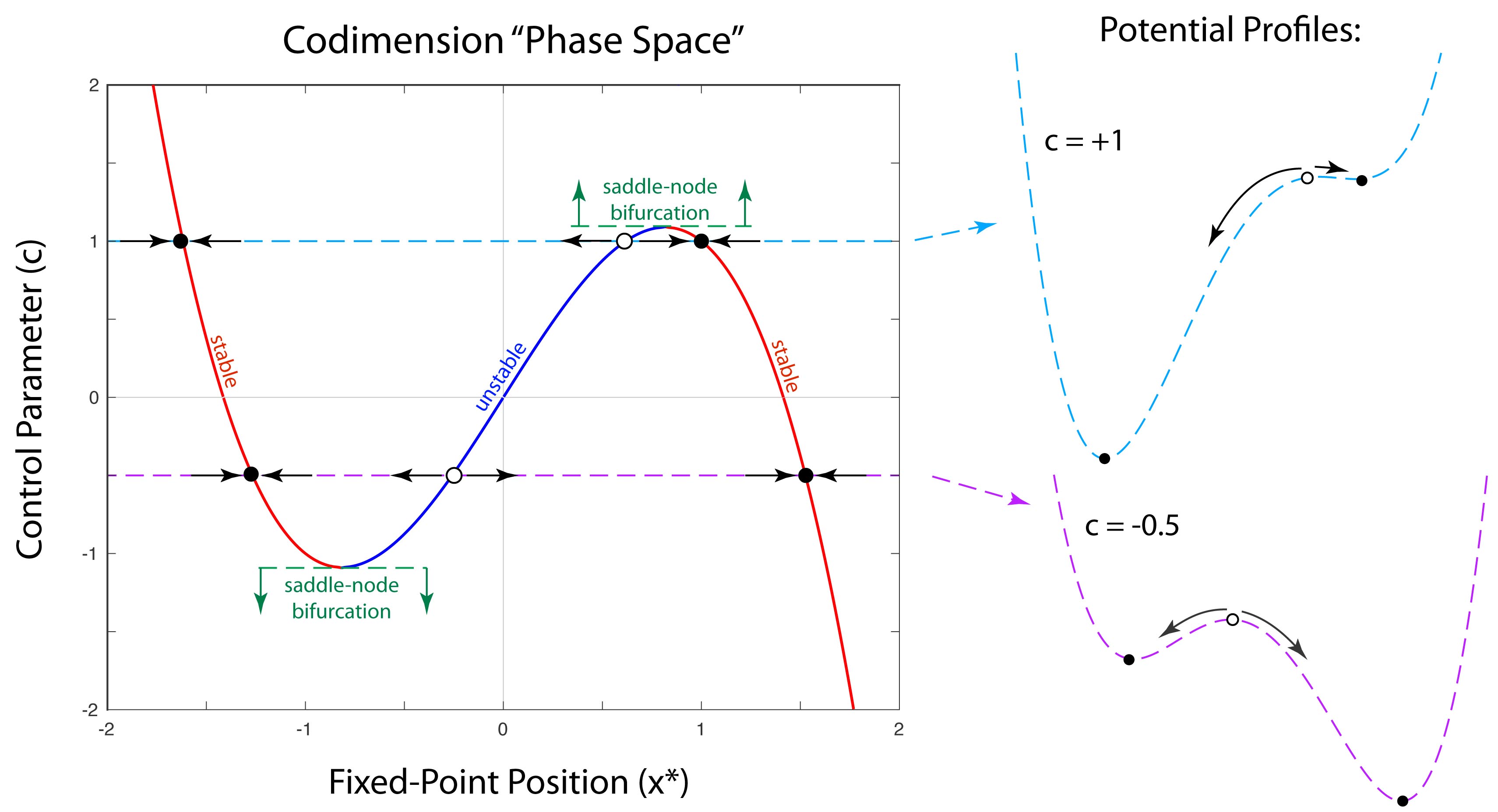
The threshold value in this example is c* = 1.05. When |c| < c* the two stable fixed points are the two minima of the double-well potential, and the unstable fixed point is the saddle between them. When |c| > c* then the single stable fixed point is the single minimum of the potential function. The saddle-node bifurcation takes its name from the fact (illustrated here) that the unstable fixed point is a saddle, and at the bifurcation the saddle point annihilates with one of the stable fixed points.

The following Python code illustrates the behavior of a biased double-well potential, with damping, in which the control parameter changes slowly with a sinusoidal time dependence.

Python Code: DWH.py

#!/usr/bin/env python3
# -*- coding: utf-8 -*-
"""
DWH.py
Created on Wed Apr 17 15:53:42 2019
@author: nolte
D. D. Nolte, Introduction to Modern Dynamics: Chaos, Networks, Space and Time, 2nd ed. (Oxford,2019)
"""

import numpy as np
from scipy import integrate
from scipy import signal
from matplotlib import pyplot as plt

plt.close('all')
T = 400
Amp = 3.5

def solve_flow(y0,c0,lim = [-3,3,-3,3]):

    def flow_deriv(x_y, t, c0):
        #"""Compute the time-derivative of a Medio system."""
        x, y = x_y

        return [y,-0.5*y - x**3 + 2*x + x*(2*np.pi/T)*Amp*np.cos(2*np.pi*t/T) + Amp*np.sin(2*np.pi*t/T)]

    tsettle = np.linspace(0,T,101)   
    yinit = y0;
    x_tsettle = integrate.odeint(flow_deriv,yinit,tsettle,args=(T,))
    y0 = x_tsettle[100,:]
    
    t = np.linspace(0, 1.5*T, 2001)
    x_t = integrate.odeint(flow_deriv, y0, t, args=(T,))
    c  = Amp*np.sin(2*np.pi*t/T)
        
    return t, x_t, c

eps = 0.0001

for loop in range(0,100):
    c = -1.2 + 2.4*loop/100 + eps;
    xc[loop]=c
    
    coeff = [-1, 0, 2, c]
    y = np.roots(coeff)
    
    xtmp = np.real(y[0])
    ytmp = np.real(y[1])
    
    X[loop] = np.min([xtmp,ytmp])
    Y[loop] = np.max([xtmp,ytmp])
    Z[loop]= np.real(y[2])


plt.figure(1)
lines = plt.plot(xc,X,xc,Y,xc,Z)
plt.setp(lines, linewidth=0.5)
plt.show()
plt.title('Roots')

y0 = [1.9, 0]
c0 = -2.

t, x_t, c = solve_flow(y0,c0)
y1 = x_t[:,0]
y2 = x_t[:,1]

plt.figure(2)
lines = plt.plot(t,y1)
plt.setp(lines, linewidth=0.5)
plt.show()
plt.ylabel('X Position')
plt.xlabel('Time')

plt.figure(3)
lines = plt.plot(c,y1)
plt.setp(lines, linewidth=0.5)
plt.show()
plt.ylabel('X Position')
plt.xlabel('Control Parameter')
plt.title('Hysteresis Figure')

Further Reading:

D. D. Nolte, Introduction to Modern Dynamics: Chaos, Networks, Space and Time (2nd Edition) (Oxford University Press, 2019)

The Pendulum Lab

Georg Duffing’s Equation

Although coal and steam launched the industrial revolution, gasoline and controlled explosions have sustained it for over a century.  After early precursors, the internal combustion engine that we recognize today came to life in 1876 from the German engineers Otto and Daimler with later variations by Benz and Diesel.  In the early 20th century, the gasoline engine was replacing coal and oil in virtually all mobile conveyances and had become a major industry attracting the top mechanical engineering talent.  One of those talents was the German engineer Georg Duffing (1861 – 1944) whose unlikely side interest in the quantum mechanics revolution brought him to Berlin to hear lectures by Max Planck, where he launched his own revolution in nonlinear oscillators.

The publication of this highly academic book by a nonacademic would establish Duffing as the originator of one of the most iconic oscillators in modern dynamics.

An Academic Non-Academic

Georg Duffing was born in 1861 in the German town of Waldshut on the border with Switzerland north of Zurich.  Within a year the family moved to Mannheim near Heidelberg where Georg received a good education in mathematics as well as music.  His mathematical interests attracted him to engineering, and he built a reputation that led to an invitation to work at Westinghouse in the United States in 1910.  When he returned to Germany he set himself up as a consultant and inventor with the freedom to move where he wished.  In early 1913 he wished to move to Berlin where Max Planck was lecturing on the new quantum mechanics at the University.  He was always searching for new knowledge, and sitting in on Planck’s lectures must have made him feel like he was witnessing the beginnings of a new era.            

At that time Duffing was interested in problems related to brakes, gears and engines.  In particular, he had become fascinated by vibrations that often were the limiting factors in engine performance.  He stripped the problem of engine vibration down to its simplest form, and he began a careful and systematic study of nonlinear oscillations.  While in Berlin, he had became acquainted with Prof. Meyer at the University who had a mechanical engineering laboratory.  Meyer let Duffing perform his experiments in the lab on the weekends, sometime accompanied by his eldest daughter.  By 1917 he had compiled a systematic investigation of various nonlinear effects in oscillators and had written a manuscript that collected all of this theoretical and experimental work.  He extended this into a small book that he published with Vieweg & Sohn in 1918 to be purchased for a price of 5 Deutsch Marks [1].   The publication of this highly academic book by a nonacademic would establish Duffing as the originator of one of the most iconic oscillators in modern dynamics.

Fig. 1 Cover of Duffing’s 1918 publication on nonlinear oscillators.

Duffing’s Nonlinear Oscillator

The mathematical and technical focus of Duffing’s book was low-order nonlinear corrections to the linear harmonic oscillator.  In one case, he considered a spring that either became stiffer or softer as it stretched.  This happens when a cubic term is added to the usual linear Hooke’s law.  In another case, he considered a spring that was stiffer in one direction than another, making the stiffness asymmetric.  This happens when a quadratic term is added.  These terms are shown in Fig. 2 from Duffing’s book.  The top equation is a free oscillation, and the bottom equation has a harmonic forcing function.  These were the central equations that Duffing explored, plus the addition of damping that he considered in a later chapter as shown in Fig. 3. The book lays out systematically, chapter by chapter, approximate and series solutions to the nonlinear equations, and in special cases described analytically exact solutions (such as for the nonlinear pendulum).

Fig. 2 Duffing’s equations without damping for free oscillation and driven oscillation with quadratic (producing an asymmetric potential) and cubic (producing stiffening or softening) corrections to the spring force.
Fig. 3 Inclusion of damping in the case with cubic corrections to the spring force.

Duffing was a practical engineer as well as a mathematical one, and he built experimental systems to test his solutions.  An engineering drawing of his experimental test apparatus is shown in Fig. 4. The small test pendulum is at S in the figure. The large pendulum at B is the drive pendulum, chosen to be much heavier than the test pendulum so that it can deliver a steady harmonic force through spring F1 to the test system. The cubic nonlinearity of the test system was controlled through the choice of the length of the test pendulum, and the quadratic nonlinearity (the asymmetry) was controlled by allowing the equilibrium angle to be shifted from vertical. The relative strength of the quadratic and cubic terms was adjusted by changing the position of the mass at G. Duffing derived expressions for all the coefficients of the equations in Fig. 1 in terms of experimentally-controlled variables. Using this apparatus, Duffing verified to good accuracy his solutions for various special cases.

Fig. 4 Duffing’s experimental system he used to explore and verify his equations and solutions.

           Duffing’s book is a masterpiece of careful systematic investigation, beginning in general terms, and then breaking the problem down into its special cases, finding solutions for each one with accurate experimental verifications. These attributes established the importance of this little booklet in the history of science and technology, but because it was written in German, most of the early citations were by German scientists.  The first use of Duffing’s name associated to the nonlinear oscillator problem occurred in 1928 [2], as was the first reference to him in a work in English in a book by Timoshenko [3].  The first use of the phrase “Duffing Equation” specifically to describe an oscillator with a linear and cubic restoring force was in 1942 in a series of lectures presented at Brown University [4], and this nomenclature had become established by the end of that decade [5].  Although Duffing had spent considerable attention in his book to the quadratic term for an asymmetric oscillator, the term “Duffing Equation” now refers to the stiffening and softening problem rather than to the asymmetric problem.

Fig. 5 The Duffing equation is generally expressed as a harmonic oscillator (first three terms plus the harmonic drive) modified by a cubic nonlinearity and driven harmonically.

Duffing Rediscovered

Nonlinear oscillations remained mainly in the realm of engineering for nearly half a century, until a broad spectrum of physical scientists began to discover deep secrets hiding behind the simple equations.  In 1963 Edward Lorenz (1917 – 2008) of MIT published a paper that showed how simple nonlinearities in three equations describing the atmosphere could produce a deterministic behavior that appeared to be completely chaotic.  News of this paper spread as researchers in many seemingly unrelated fields began to see similar signatures in chemical reactions, turbulence, electric circuits and mechanical oscillators.  By 1972 when Lorenz was invited to give a talk on the “Butterfly Effect” the science of chaos was emerging as new frontier in physics, and in 1975 it was given its name “chaos theory” by James Yorke (1941 – ).  By 1976 it had become one of the hottest new areas of science. 

        Through the period of the emergence of chaos theory, the Duffing oscillator was known to be one of the archetypical nonlinear oscillators.  A particularly attractive aspect of the general Duffing equations is the possibility of studying a “double-well” potential.  This happens when the “alpha” in the equation in Fig. 5 is negative and the “beta” is positive.  The double-well potential has a long history in physics, both classical and modern, because it represents a “two-state” system that exhibits bistability, bifurcations, and hysteresis.  For a fixed “beta” the potential energy as a function of “alpha” is shown in Fig. 6.  The bifurcation cascades of the double-well Duffing equation was investigated by Phillip Holmes (1945 – ) in 1976 [6], and the properties of the strange attractor were demonstrated in 1978 [7] by Yoshisuke Ueda (1936 – ).  Holmes, and others, continued to do detailed work on the chaotic properties of the Duffing oscillator, helping to make it one of the most iconic systems of chaos theory.

Fig. 6 Potential energy of the Duffing Oscillator. The position variable is x, and changing alpha is along the other axis. For positive beta and alpha the potential is a quartic. For positive beta and negative alpha the potential is a double well.

Python Code for the Duffing Oscillator: Duffing.py

This Python code uses the simple ODE solver on the driven-damped Duffing double-well oscillator to display the configuration-space trajectories and the Poincaré map of the strange attractor. (Python code on GitHub.)

#!/usr/bin/env python3
# -*- coding: utf-8 -*-
"""
Duffing.py
Created on Wed May 21 06:03:32 2018
@author: nolte
D. D. Nolte, Introduction to Modern Dynamics: Chaos, Networks, Space and Time, 2nd ed. (Oxford,2019)
"""
import numpy as np
import matplotlib as mpl
from mpl_toolkits.mplot3d import Axes3D
from scipy import integrate
from matplotlib import pyplot as plt
from matplotlib import cm
import time
import os

plt.close('all')

# model_case 1 = Pendulum
# model_case 2 = Double Well
print(' ')
print('Duffing.py')

alpha = -1       # -1
beta = 1         # 1
delta = 0.3       # 0.3
gam = 0.15    # 0.15
w = 1
def flow_deriv(x_y_z,tspan):
    x, y, z = x_y_z
    a = y
    b = delta*np.cos(w*tspan) - alpha*x - beta*x**3 - gam*y
    c = w
    return[a,b,c]
                
T = 2*np.pi/w

px1 = np.random.rand(1)
xp1 = np.random.rand(1)
w1 = 0

x_y_z = [xp1, px1, w1]

# Settle-down Solve for the trajectories
t = np.linspace(0, 2000, 40000)
x_t = integrate.odeint(flow_deriv, x_y_z, t)
x0 = x_t[39999,0:3]

tspan = np.linspace(1,20000,400000)
x_t = integrate.odeint(flow_deriv, x0, tspan)
siztmp = np.shape(x_t)
siz = siztmp[0]

y1 = x_t[:,0]
y2 = x_t[:,1]
y3 = x_t[:,2]
    
plt.figure(2)
lines = plt.plot(y1[1:2000],y2[1:2000],'ko',ms=1)
plt.setp(lines, linewidth=0.5)
plt.show()

for cloop in range(0,3):

#phase = np.random.rand(1)*np.pi;
    phase = np.pi*cloop/3

    repnum = 5000
    px = np.zeros(shape=(2*repnum,))
    xvar = np.zeros(shape=(2*repnum,))
    cnt = -1
    testwt = np.mod(tspan-phase,T)-0.5*T;
    last = testwt[1]
    for loop in range(2,siz):
        if (last < 0)and(testwt[loop] > 0):
            cnt = cnt+1
            del1 = -testwt[loop-1]/(testwt[loop] - testwt[loop-1])
            px[cnt] = (y2[loop]-y2[loop-1])*del1 + y2[loop-1]
            xvar[cnt] = (y1[loop]-y1[loop-1])*del1 + y1[loop-1]
            last = testwt[loop]
        else:
            last = testwt[loop]
 
    plt.figure(3)
    if cloop == 0:
        lines = plt.plot(xvar,px,'bo',ms=1)
    elif cloop == 1:
        lines = plt.plot(xvar,px,'go',ms=1)
    else:
        lines = plt.plot(xvar,px,'ro',ms=1)
        
    plt.show()

plt.savefig('Duffing')
Fig. 7 Strange attractor of the double-well Duffing equation for three selected phases.


Read all the stories behind the history of chaos theory, in Galileo Unbound from Oxford Press:


References

[1] G. Duffing, Erzwungene Schwingungen bei veranderlicher Eigenfrequenz und ihre technische Bedeutung, Vieweg & Sohn, Braunschweig, 1918.

[2] Lachmann, K. “Duffing’s vibration problem.” Mathematische Annalen 99: 479-492. (1928)

[3] S. Timoshenko, Vibration Problems in Engineering, D. Van Nostrand Company, Inc.,New York, 1928.

[4] K.O. Friedrichs, P. Le Corbeiller, N. Levinson, J.J. Stoker, Lectures on Non-Linear Mechanics delivered at Brown University, New York, 1942.

[5] Kovacic, I. and M. J. Brennan, Eds. The Duffing Equation: Nonlinear Oscillators and their Behavior. Chichester, United Kingdom, Wiley. (2011)

[6] Holmes, P. J. and D. A. Rand. “Bifurcations of Duffings Equation – Application of Catastrophe Theory.” Journal of Sound and Vibration 44(2): 237-253. (1976)

[7] Ueda, Y. “Randomly Transitional Phenomena in the System Governed by Duffings Equation.” Journal of Statistical Physics 20(2): 181-196. (1979)