Everyone who has taken classes in physics or engineering knows that the most magical of all vector identities (and there are so many vector identities) are Green’s theorem in 2D, and Stokes’ and Gauss’ theorem in 3D.  These theorems have the magical ability to take an integral over some domain and replace it with a simpler integral over the boundary of the domain.  For instance, the vector form of Stokes’ theorem in 3D is

for the curl of a vector field, where S is the surface domain, and C is the closed loop surrounding the domain.

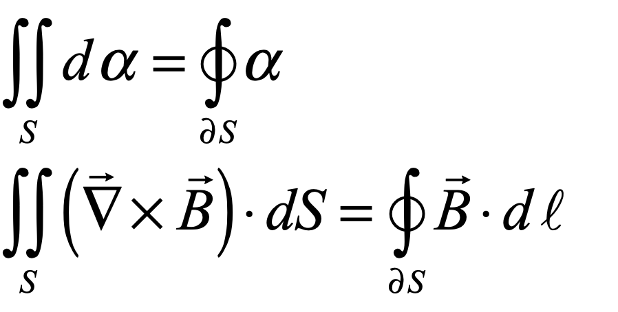
Maybe the most famous application of these theorems is to convert Maxwell’s equations of electromagnetism from their differential form to their integral form.  For instance, we can start with the differential version for the curl of the B-field and integrate over a surface

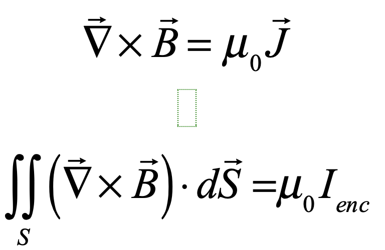
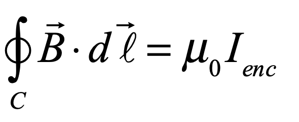
then applying Stokes’ theorem in 3D (or Green’s theorem in 2D), that converts from the two-dimensional surface integral to a one-dimensional integral around a closed loop bounding the area integral domain yields the integral form of Ampere’s law

Stokes’ theorem has the important property that it converts a high-dimensional integral into a lower-dimensional integral over the closed boundary of the original domain. Stokes’ theorem in component form is

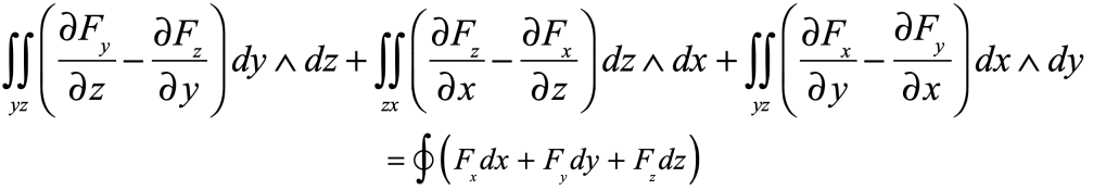
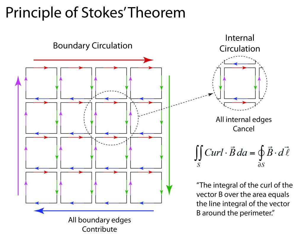
where the “hat” symbol is Grassmann’s wedge product (see below). In the case of Green’s theorem in 2D, the principle is easy to explain by the oriented vector character of the integrals and the notion of dividing a domain into small elements with oriented edges. In the case of nonzero circulation, all internal edges of smaller regions cancel pairwise until the outer boundary is reached, where a macroscopic circulation persists along all the outer edges. Similarly in Gauss’ theorem in 3D, the flux of a vector through the face of one element is equal and opposite to the flux through the adjacent element, canceling out pairwise until the outer boundary is reached and the net flux is finite summed over the outer elements. This general property of pairwise cancelation on adjacent subdomains until the outer boundary is reached is the general property of Stokes’ theorem that can be extended to space of any dimensions or onto general manifolds that do not need to be Euclidean.

George Stokes and the Cambridge Tripos

Since 1824, the mathematics course at Cambridge University has held a yearly exam called the Tripos to identify the top graduating mathematics student.  The winner of the contest is called the Senior Wrangler, and in the 1800’s the Senior Wrangler received a level of public fame and admiration for intellectual achievement that is somewhat like the fame reserved today for star athletes.  Famous Senior Wranglers include George Airy, John Herschel, Arthur Cayley, Lord Rayleigh, Arthur Eddington, J. E. Littlewood, Peter Guthrie Tait and Joseph Larmor.

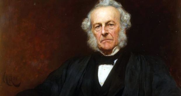
            In his second year at Cambridge, Stokes had begun studying under William Hopkins (1793 – 1866), and in 1841 George Stokes became Senior Wrangler the same year he won the Smith’s Prize in mathematics.  The Tripos tested primarily on bookwork, while the Smith’s Prize tested on originality.  To achieve top scores on both designated the student as the most capable and creative mathematician of his class.  Stokes was immediately offered a fellowship at Pembroke College allowing him to teach and study whatever he willed. Within eight years he was chosen for the Lucasian Chair of Mathematics. The Lucasian Chair of Mathematics at Cambridge is one of the most famous academic chairs in the world.  The first Lucasian professor was Isaac Barrow in 1664 followed by Isaac Newton who held the post for 33 years.  Other famous Lucasian professors were George Airy, Charles Babbage, Joseph Larmor, Paul Dirac as well as Stephen Hawking. Among the many fields that Stokes made important contributions was hydrodynamics where he derived Stokes’ Law of Drag.

In 1854 Stokes was one of the Cambridge professors setting exam questions for the Tripos. In a letter that William Thompson (later Lord Kelvin) wrote Stokes, he suggested putting on the exam the task of extending Green’s Theorem to three dimensions and proving the theorem, and Stokes obliged. That year the Tripos consisted of 16 papers spread over 8 days, totaling over 40 hours of effort on 211 questions. One of the candidates for Senior Wrangler that year was James Clerk Maxwell, but he was narrowly beaten out by Edward Routh (1831 – 1907). Routh became famous, but not as famous as Maxwell who later applied Stokes’ Theorem to derive the equations of electrodynamics.

The Fundamental Theorem of Calculus

One of the first and simplest theorems that any student of intro calculus is taught is the Fundamental Theorem of Calculus

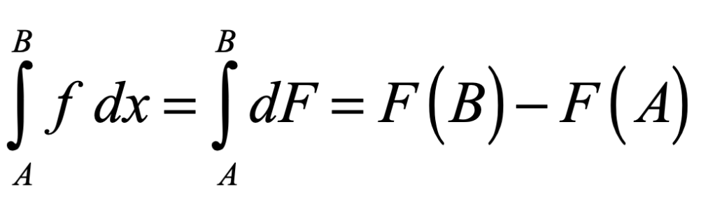
where F is called the “antiderivative” of the function f . The interpretation of the Fundamental Theorem is extremely simple:  The integral of a function over a domain is equal to its antiderivative evaluated at the boundary of the domain.  Generalizing this theorem a bit, it says that evaluating an integral over a domain is the same thing as evaluating a lower-dimensional quantity over the boundary of the domain.  The Fundamental Theorem of Calculus sounds a lot like Green’s Theorem or Stokes’ Theorem!  And in fact, they are all part of the same principle.  To understand this principle, we have to look into differential forms and the use of Grassmann’s wedge product and exterior algebra (the subject of my previous blog post).

Differential Forms

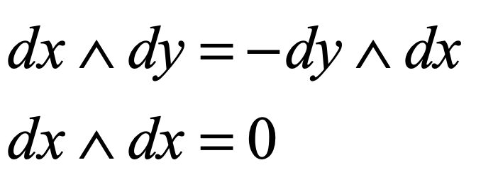
Just as in the case of the exterior algebra , the fundamental identities defined for differential forms are given by

A differential 1-form α and a differential 2-form β can be expressed as

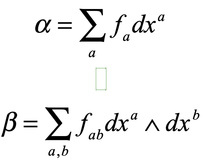
The key to understanding why the wedge product shows up in this definition is to recognize that the operation of producing a product of differentials is only defined for the wedge product.  Within the language of differential forms, the symbol dxdy has no meaning, despite the fact that this symbol shows up routinely when integrating.  In fact, integrals that use the expression dxdy are ambiguous, because the oriented surface must be inferred from the context of the integral rather than given.  This is why integration over multiple variables should actually be performed using differential forms, though it is rarely (or never) stated in lower-level calculus classes.

Integration of Differential Forms

Line integrals, as in the Fundamental Theorem of Calculus, are obvious and unique.  However, as soon as we move to integrals over areas, the wedge product is needed.  This is because a general area is oriented.  If you think of a plane defined by z = 0, the surface element dxdy can be oriented along either the positive z-axis or the negative z-axis.  Which one should you take?  The answer is: don’t make the choice.  Work with differential forms, and the integral may be over dx^dy or dy^dx, depending on the exterior analysis that produced the integral in the first place.  One is the negative of the other.  You take the element as it arises from the algebra, and you cannot go wrong!

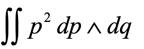
As an example, we can use differential forms to express a surface integral correctly as

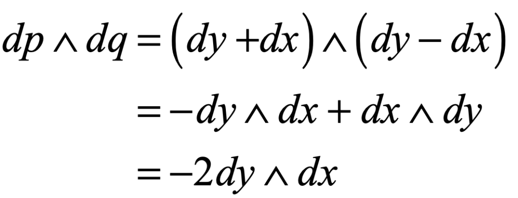
If you make the substitutions: x = (p-q)/2 and y = (p+q)/2, then dp = dx + dy and dq = dy – dx and

which yields

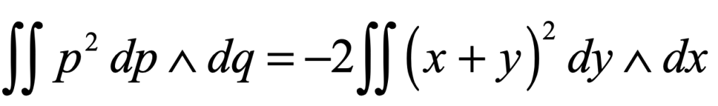
In this case, you will recognize that the factor of -2 is just the Jacobian of the transformation.  Working this way with differential forms makes transformation simple, like a book-keeping trick, and safe, so you just follow the algebra through without needing to make choices.

Exterior Differentiation

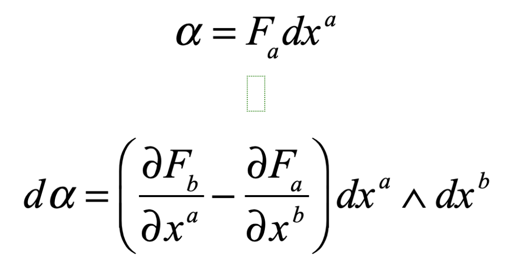
The exterior derivative of the 1-form α (defined above) is defined as

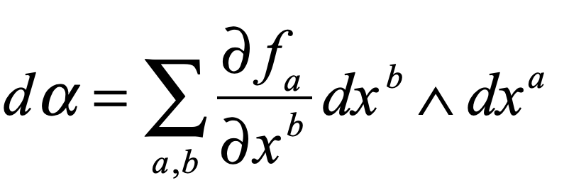
where the exterior derivative turns a differential r-form into a differential (r+1)-form.  For instance, in 3D

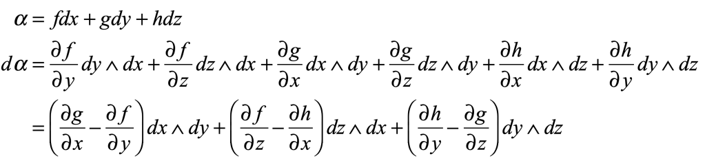
This should look very familiar to you.  If we expressly make the equivalence

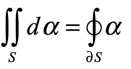
where the integral on the left is a surface integral over a domain, and the integral on the right is a line integral over a line bounding the domain, then

This is just the curl theorem (Stokes’ theorem).

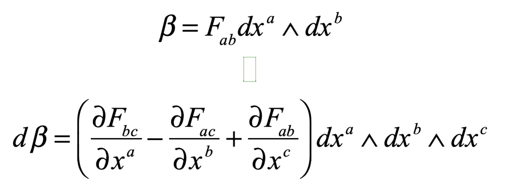
Taking the dimension up one notch, consider the differential 2-form β where

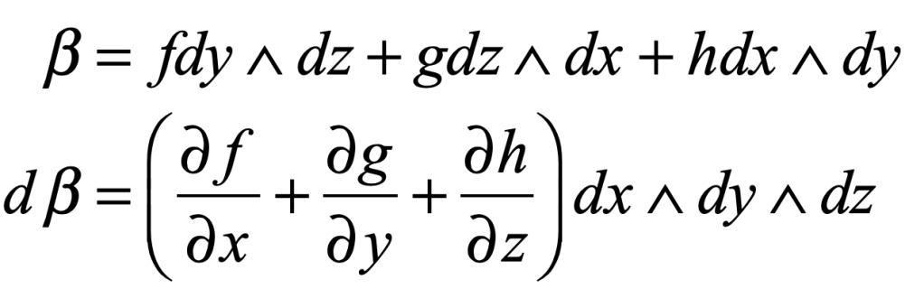
This again looks very familiar, and if we write down the equivalence

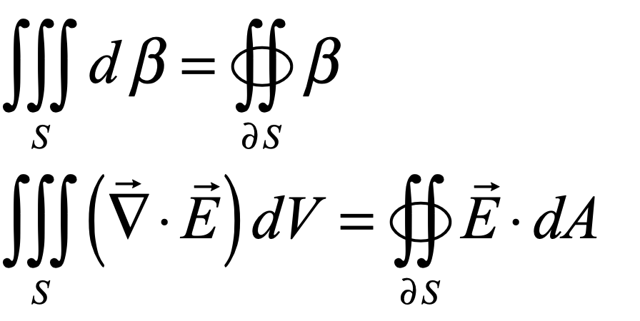
then we immediately have the divergence theorem.

We can even find other vector identities using these differential forms.  For instance, if we start with a 2-form expressed as

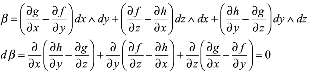
then we have proven the vector identity

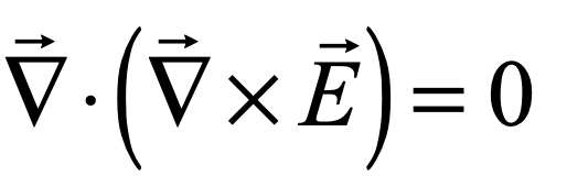
stating that the divergence of a curl must vanish.  This is like playing games with simple algebra to prove profound theorems in vector calculus!

Stokes’ Theorem in Higher Dimensions

The power of differential forms is their ability to generalize automatically to higher dimensions. The differential 1-form can have any number of indices for multiple dimensions, and exterior differentiation yields the familiar curl theorem in any number of dimensions

But the differential 2-form in 4D yields to exterior differentiation to give a mixed expression that is neither a curl nor a divergence

The differential 3-form in 4D under exterior differentiation yields the 4D divergence

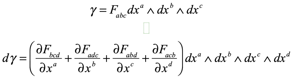
although the orientations of the 3D boundary elements must be chosen appropriately.

Differential Forms in 4D Electromagnetics

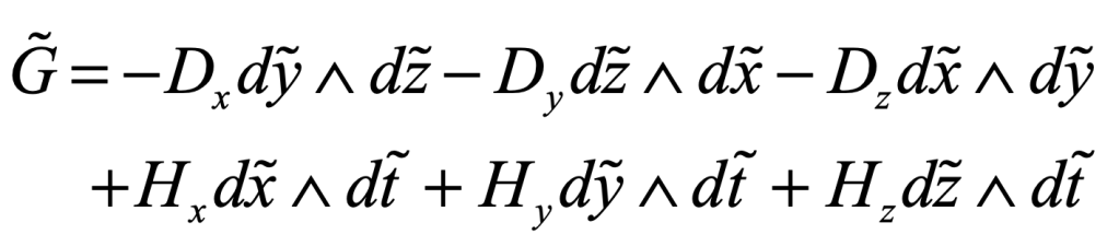
As long as we are working with differential forms and Stokes’ Theorem, let’s finish up by looking at Maxwell’s electromagnetic equations as four-dimensional equations in spacetime.  First, construct the 2-form using the displacement field D and the magnetic intensity H.

The differential of this two-form creates a lot of terms, such as

This can be simplified by collecting like terms to

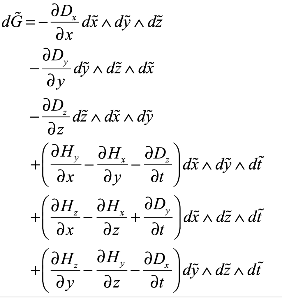
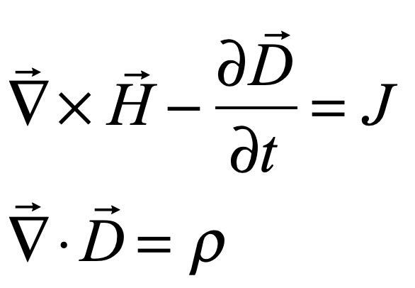
Renaming each coefficient so that

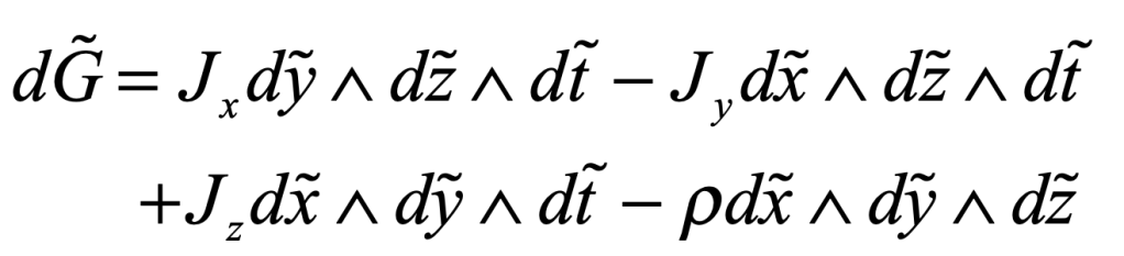
yields two of Maxwell’s equations

To find the other two Maxwell equations, start with the 1-form

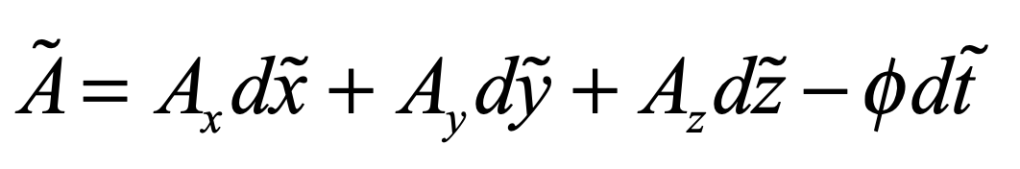
and try the derivation yourself!

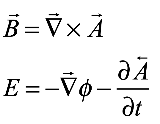
Differentiating yields a differential two-form. Then identify the curl of the vector potential as the B-field, etc., to derive the other two Maxwell equations

Bibliography

Vargas, J. G., Differential Geometry for Physicists and Mathematicians: Moving Frames and Differential Forms: From Euclid Past Riemann. 2014; p 1-293.