
In the midst of this COVID crisis (and the often botched governmental responses to it), there have been several success stories: Taiwan, South Korea, Australia and New Zealand stand out. What are the secrets to their success? First, is the willingness of the population to accept the seriousness of the pandemic and to act accordingly. Second, is a rapid and coherent (and competent) governmental response. Third, is biotechnology and the physics of ultra-sensitive biomolecule detection.
Antibody Testing
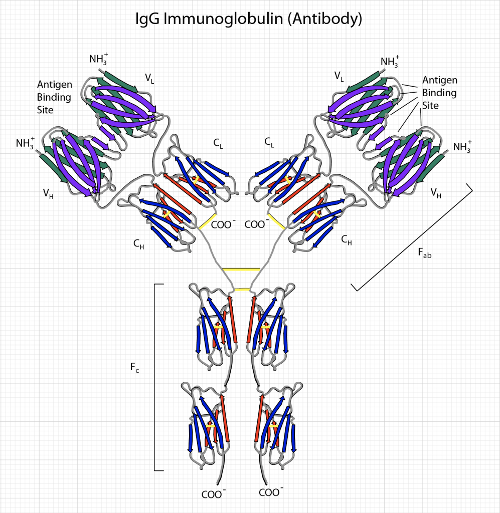
A virus consists a protein package called a capsid that surrounds polymers of coding RNA. Protein molecules on the capsid are specific to the virus and are the key to testing whether a person has been exposed to the virus. These specific molecules are called antigens, and the body produces antibodies — large biomolecules — that are rapidly evolved by the immune system and released into the blood system to recognize and bind to the antigen. The recognition and binding is highly specific (though not perfect) to the capsid proteins of the virus, so that other types of antibodies (produced to fend off other infections) tend not to bind to it. This specificity enables antibody testing.
In principle, all one needs to do is isolate the COVID-19 antigen, bind it to a surface, and run a sample of a patient’s serum (the part of the blood without the blood cells) over the same surface. If the patient has produced antibodies against the COVID-19, these antibodies will attach to the antigens stuck to the surface. After washing away the rest of the serum, what remains are anti-COVID antibodies attached to the antigens bound to the surface. The next step is to determine whether these antibodies have been bound to the surface or not.
At this stage, there are many possible alternative technologies to detecting the bound antibodies (see section below on the physics of the BioCD for one approach). A conventional detection approach is known as ELISA (Enzyme-linked immunosorbant assay). To detect the bound antibody, a secondary antibody that binds to human antibodies is added to the test well. This secondary antibody contains either a fluorescent molecular tag or an enzyme that causes the color of the well to change (kind of like how a pregnancy test causes a piece of paper to change color). If the COVID antigen binds antibodies from the patient serum, then this second antibody will bind to the first and can be detected by fluorescence or by simple color change.
The technical challenges associated with antibody assays relate to false positives and false negatives. A false positive happens when the serum is too sticky and some antibodies NOT against COVID tend to stick to the surface of the test well. This is called non-specific binding. The secondary antibodies bind to these non-specifically-bound antibodies and a color change reports a detection, when in fact no COVID-specific antibodies were there. This is a false positive — the patient had not been exposed, but the test says they were.
On the other hand, a false negative occurs when the patient serum is possibly too dilute and even though anti-COVID antibodies are present, they don’t bind sufficiently to the test well to be detectable. This is a false negative — the patient had been exposed, but the test says they weren’t. Despite how mature antibody assay technology is, false positives and false negatives are very hard to eliminate. It is fairly common for false rates to be in the range of 5% to 10% even for high-quality immunoassays. The finite accuracy of the tests must be considered when doing community planning for testing and tracking. But the bottom line is that even 90% accuracy on the test can do a lot to stop the spread of the infection. This is because of the geometry of social networks and how important it is to find and isolate the super spreaders.
Social Networks
The web of any complex set of communities and their interconnections aren’t just random. Whether in interpersonal networks, or networks of cities and states and nations, it’s like the world-wide-web where the most popular webpages get the most links. This is the same phenomenon that makes the rich richer and the poor poorer. It produces a network with a few hubs that have a large fraction of the links. A network model that captures this network topology is known as the Barabasi-Albert model for scale-free networks [1]. A scale-free network tends to have one node that has the most links, then a couple of nodes that have a little fewer links, then several more with even fewer, and so on, until there are a vary large number of nodes with just a single link each.
When it comes to pandemics, this type of network topology is both a curse and a blessing. It is a curse, because if the popular node becomes infected it tends to infect a large fraction of the rest of the network because it is so linked in. But it is a blessing, because if that node can be identified and isolated from the rest of the network, then the chance of the pandemic sweeping across the whole network can be significantly reduced. This is where testing and contact tracing becomes so important. You have to know who is infected and who they are connected with. Only then can you isolate the central nodes of the network and make a dent in the pandemic spread.
An example of a Barabasi-Albert network is shown in Fig. 2 having 128 nodes. Some nodes have many links out (and in) the number of links connecting a node is called the node degree. There are several nodes of very high degree (a degree around 25 in this case) but also very many nodes that have only a single link. It’s the high-degree nodes that matter in a pandemic. If they get infected, then they infect almost the entire network. This scale-free network structure emphasizes the formation of central high-degree nodes. It tends to hold for many social networks, but also can stand for cities across a nation. A city like New York has links all over the country (by flights), while my little town of Lafayette IN might be modeled by a single link to Indianapolis. That same scaling structure is seen across many scales from interactions among nations to interactions among citizens in towns.

Isolating the Super Spreaders
In the network of nodes in Fig. 2, each node can be considered as a “compartment” in a multi-compartment SIR model (see my previous blog for the two-compartment SIR model of COVID-19). The infection of each node depends on the SIR dynamics of that node, plus the infections coming in from links other infected nodes. The equations of the dynamics for each node are

where Aab is the adjacency matrix where self-connection is allowed (infection dynamics within a node) and the sums go over all the nodes of the network. In this model, the population of each node is set equal to the degree ka of the node. The spread of the pandemic across the network depends on the links and where the infection begins, but the overall infection is similar to the simple SIR model for a given average network degree
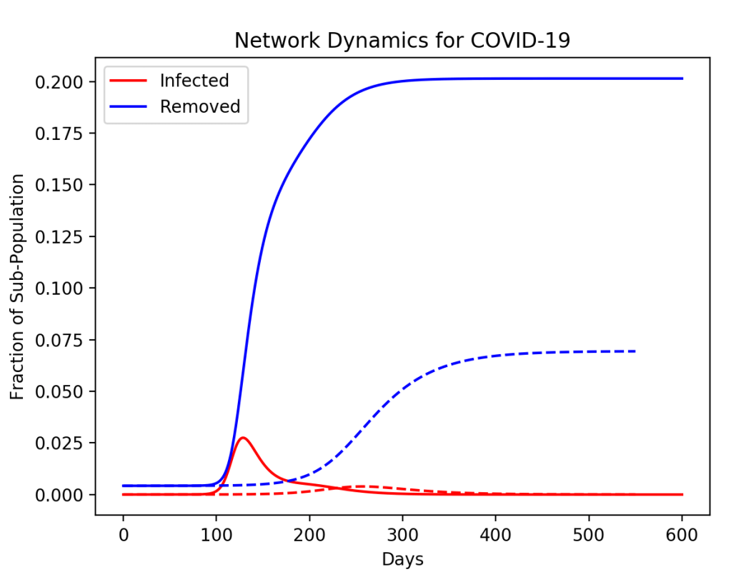
However, if the pandemic starts, but then the highest-degree node (the super spreader) is isolated (by testing and contact tracing), then the saturation of the disease across the network can be decreased in a much greater proportion than simply given by the population of the isolated node. For instance, in the simulation in Fig. 3, a node of degree 20 is removed at 50 days. The fraction of the population that is isolated is only 10%, yet the saturation of the disease across the whole network is decreased by more than a factor of 2.
In a more realistic model with many more nodes, and full testing to allow the infected nodes and their connections to be isolated, the disease can be virtually halted. This is what was achieved in Taiwan and South Korea. The question is why the United States, with its technologically powerful companies and all their capabilities, was so unprepared or unwilling to achieve the same thing.
Python Code: NetSIRSF.py
#!/usr/bin/env python3
# -*- coding: utf-8 -*-
"""
NetSIRSF.py
Created on Sat May 11 08:56:41 2019
@author: nolte
D. D. Nolte, Introduction to Modern Dynamics: Chaos, Networks, Space and Time, 2nd ed. (Oxford,2019)
"""

# https://www.python-course.eu/networkx.php
# https://networkx.github.io/documentation/stable/tutorial.html
# https://networkx.github.io/documentation/stable/reference/functions.html

import numpy as np
from scipy import integrate
from matplotlib import pyplot as plt
import networkx as nx
import time
from random import random

tstart = time.time()

plt.close('all')

betap = 0.014;
mu = 0.13;

print('beta = ',betap)
print('betap/mu = ',betap/mu)


N = 128      # 50


facoef = 2
k = 1
nodecouple = nx.barabasi_albert_graph(N, k, seed=None)

indhi = 0
deg = 0
for omloop in nodecouple.node:
    degtmp = nodecouple.degree(omloop)
    if degtmp > deg:
        deg = degtmp
        indhi = omloop
print('highest degree node = ',indhi)
print('highest degree = ',deg)

plt.figure(1)
colors = [(random(), random(), random()) for _i in range(10)]
nx.draw_circular(nodecouple,node_size=75, node_color=colors)
print(nx.info(nodecouple))

# function: omegout, yout = coupleN(G)
def coupleN(G,tlim):

    # function: yd = flow_deriv(x_y)
    def flow_deriv(x_y,t0):

        N = np.int(x_y.size/2)
        yd = np.zeros(shape=(2*N,))
        ind = -1
        for omloop in G.node:
            ind = ind + 1
            temp1 = -mu*x_y[ind] + betap*x_y[ind]*x_y[N+ind]
            temp2 =  -betap*x_y[ind]*x_y[N+ind]
            linksz = G.node[omloop]['numlink']
            for cloop in range(linksz):
                cindex = G.node[omloop]['link'][cloop]
                indx = G.node[cindex]['index']
                g = G.node[omloop]['coupling'][cloop]

                temp1 = temp1 + g*betap*x_y[indx]*x_y[N+ind]
                temp2 = temp2 - g*betap*x_y[indx]*x_y[N+ind]

            yd[ind] = temp1
            yd[N+ind] = temp2

        return yd
    # end of function flow_deriv(x_y)
    x0 = x_y
    t = np.linspace(0,tlim,tlim)      # 600  300
    y = integrate.odeint(flow_deriv, x0, t)

    return t,y
    # end of function: omegout, yout = coupleN(G)

lnk = np.zeros(shape = (N,), dtype=int)
ind = -1
for loop in nodecouple.node:
    ind = ind + 1
    nodecouple.node[loop]['index'] = ind
    nodecouple.node[loop]['link'] = list(nx.neighbors(nodecouple,loop))
    nodecouple.node[loop]['numlink'] = len(list(nx.neighbors(nodecouple,loop)))
    lnk[ind] = len(list(nx.neighbors(nodecouple,loop)))

gfac = 0.1

ind = -1
for nodeloop in nodecouple.node:
    ind = ind + 1
    nodecouple.node[nodeloop]['coupling'] = np.zeros(shape=(lnk[ind],))
    for linkloop in range (lnk[ind]):
        nodecouple.node[nodeloop]['coupling'][linkloop] = gfac*facoef

x_y = np.zeros(shape=(2*N,))
for loop in nodecouple.node:
    x_y[loop]=0
    x_y[N+loop]=nodecouple.degree(loop)
    #x_y[N+loop]=1
x_y[N-1 ]= 0.01
x_y[2*N-1] = x_y[2*N-1] - 0.01
N0 = np.sum(x_y[N:2*N]) - x_y[indhi] - x_y[N+indhi]
print('N0 = ',N0)

tlim0 = 600
t0,yout0 = coupleN(nodecouple,tlim0)                           # Here is the subfunction call for the flow


plt.figure(2)
plt.yscale('log')
plt.gca().set_ylim(1e-3, 1)
for loop in range(N):
    lines1 = plt.plot(t0,yout0[:,loop])
    lines2 = plt.plot(t0,yout0[:,N+loop])
    lines3 = plt.plot(t0,N0-yout0[:,loop]-yout0[:,N+loop])

    plt.setp(lines1, linewidth=0.5)
    plt.setp(lines2, linewidth=0.5)
    plt.setp(lines3, linewidth=0.5)


Itot = np.sum(yout0[:,0:127],axis = 1) - yout0[:,indhi]
Stot = np.sum(yout0[:,128:255],axis = 1) - yout0[:,N+indhi]
Rtot = N0 - Itot - Stot
plt.figure(3)
#plt.plot(t0,Itot,'r',t0,Stot,'g',t0,Rtot,'b')
plt.plot(t0,Itot/N0,'r',t0,Rtot/N0,'b')
#plt.legend(('Infected','Susceptible','Removed'))
plt.legend(('Infected','Removed'))
plt.hold

# Repeat but innoculate highest-degree node
x_y = np.zeros(shape=(2*N,))
for loop in nodecouple.node:
    x_y[loop]=0
    x_y[N+loop]=nodecouple.degree(loop)
    #x_y[N+loop]=1
x_y[N-1] = 0.01
x_y[2*N-1] = x_y[2*N-1] - 0.01
N0 = np.sum(x_y[N:2*N]) - x_y[indhi] - x_y[N+indhi]

tlim0 = 50
t0,yout0 = coupleN(nodecouple,tlim0)


# remove all edges from highest-degree node
ee = list(nodecouple.edges(indhi))
nodecouple.remove_edges_from(ee)
print(nx.info(nodecouple))

#nodecouple.remove_node(indhi)
lnk = np.zeros(shape = (N,), dtype=int)
ind = -1
for loop in nodecouple.node:
    ind = ind + 1
    nodecouple.node[loop]['index'] = ind
    nodecouple.node[loop]['link'] = list(nx.neighbors(nodecouple,loop))
    nodecouple.node[loop]['numlink'] = len(list(nx.neighbors(nodecouple,loop)))
    lnk[ind] = len(list(nx.neighbors(nodecouple,loop)))

ind = -1
x_y = np.zeros(shape=(2*N,))
for nodeloop in nodecouple.node:
    ind = ind + 1
    nodecouple.node[nodeloop]['coupling'] = np.zeros(shape=(lnk[ind],))
    x_y[ind] = yout0[tlim0-1,nodeloop]
    x_y[N+ind] = yout0[tlim0-1,N+nodeloop]
    for linkloop in range (lnk[ind]):
        nodecouple.node[nodeloop]['coupling'][linkloop] = gfac*facoef


tlim1 = 500
t1,yout1 = coupleN(nodecouple,tlim1)

t = np.zeros(shape=(tlim0+tlim1,))
yout = np.zeros(shape=(tlim0+tlim1,2*N))
t[0:tlim0] = t0
t[tlim0:tlim1+tlim0] = tlim0+t1
yout[0:tlim0,:] = yout0
yout[tlim0:tlim1+tlim0,:] = yout1


plt.figure(4)
plt.yscale('log')
plt.gca().set_ylim(1e-3, 1)
for loop in range(N):
    lines1 = plt.plot(t,yout[:,loop])
    lines2 = plt.plot(t,yout[:,N+loop])
    lines3 = plt.plot(t,N0-yout[:,loop]-yout[:,N+loop])

    plt.setp(lines1, linewidth=0.5)
    plt.setp(lines2, linewidth=0.5)
    plt.setp(lines3, linewidth=0.5)


Itot = np.sum(yout[:,0:127],axis = 1) - yout[:,indhi]
Stot = np.sum(yout[:,128:255],axis = 1) - yout[:,N+indhi]
Rtot = N0 - Itot - Stot
plt.figure(3)
#plt.plot(t,Itot,'r',t,Stot,'g',t,Rtot,'b',linestyle='dashed')
plt.plot(t,Itot/N0,'r',t,Rtot/N0,'b',linestyle='dashed')
#plt.legend(('Infected','Susceptible','Removed'))
plt.legend(('Infected','Removed'))
plt.xlabel('Days')
plt.ylabel('Fraction of Sub-Population')
plt.title('Network Dynamics for COVID-19')
plt.show()
plt.hold()

elapsed_time = time.time() - tstart
print('elapsed time = ',format(elapsed_time,'.2f'),'secs')
Caveats and Disclaimers
No effort in the network model was made to fit actual disease statistics. In addition, the network in Figs. 2 and 3 only has 128 nodes, and each node was a “compartment” that had its own SIR dynamics. This is a coarse-graining approach that would need to be significantly improved to try to model an actual network of connections across communities and states. In addition, isolating the super spreader in this model would be like isolating a city rather than an individual, which is not realistic. The value of a heuristic model is to gain a physical intuition about scales and behaviors without being distracted by details of the model.
Postscript: Physics of the BioCD
Because antibody testing has become such a point of public discussion, it brings to mind a chapter of my own life that was closely related to this topic. About 20 years ago my research group invented and developed an antibody assay called the BioCD [2]. The “CD” stood for “compact disc”, and it was a spinning-disk format that used laser interferometry to perform fast and sensitive measurements of antibodies in blood. We launched a start-up company called QuadraSpec in 2004 to commercialize the technology for large-scale human disease screening.
A conventional compact disc consists of about a billion individual nulling interferometers impressed as pits into plastic. When the read-out laser beam straddles one of the billion pits, it experiences a condition of perfect destructive interferences — a zero. But when it was not shining on a pit it experiences high reflection — a one. So as the laser scans across the surface of the disc as it spins, a series of high and low reflections read off bits of information. Because the disc spins very fast, the data rate is very high, and a billion bits can be read in a matter of minutes.
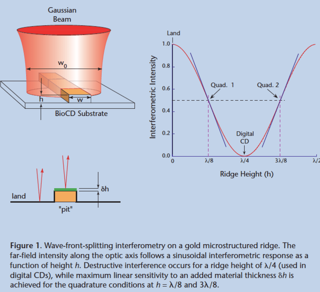
The idea struck me in late 1999 just before getting on a plane to spend a weekend in New York City: What if each pit were like a test tube, so that instead of reading bits of ones and zeros it could read tiny amounts of protein? Then instead of a billion ones and zeros the disc could read a billion protein concentrations. But nulling interferometers are the least sensitive way to measure something sensitively because it operates at a local minimum in the response curve. The most sensitive way to do interferometry is in the condition of phase quadrature when the signal and reference waves are ninety-degrees out of phase and where the response curve is steepest, as in Fig. 4 . Therefore, the only thing you need to turn a compact disc from reading ones and zeros to proteins is to reduce the height of the pit by half. In practice we used raised ridges of gold instead of pits, but it worked in the same way and was extremely sensitive to the attachment of small amounts of protein.
This first generation BioCD was literally a work of art. It was composed of a radial array of gold strips deposited on a silicon wafer. We were approached in 2004 by an art installation called “Massive Change” that was curated by the Vancouver Art Museum. The art installation travelled to Toronto and then to the Museum of Contemporary Art in Chicago, where we went to see it. Our gold-and-silicon BioCD was on display in a section on art in technology.
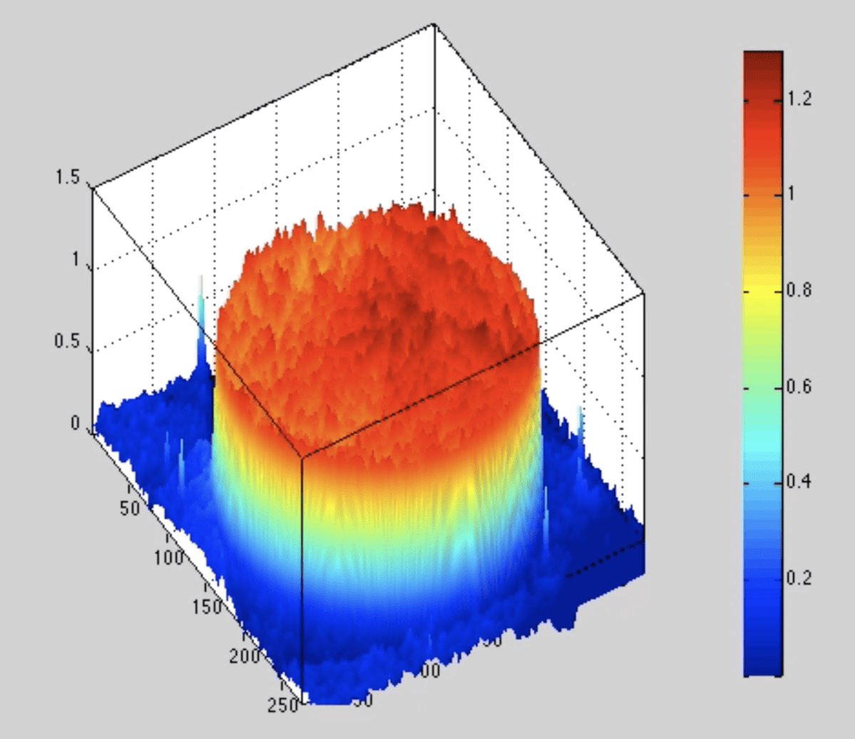
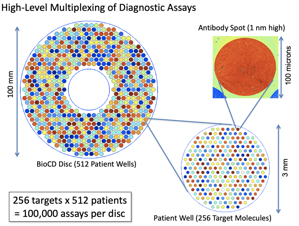
The next-gen BioCDs were much simpler, consisting simply of oxide layers on silicon wafers, but they were much more versatile and more sensitive. An optical scan of a printed antibody spot on a BioCD is shown in Fig. 5 The protein height is only about 1 nanometer (the diameter of the spot is 100 microns). Interferometry can measure a change in the height of the spot (caused by binding antibodies from patient serum) by only about 10 picometers averaged over the size of the spot. This exquisite sensitivity enabled us to detect tiny fractions of blood-born antigens and antibodies at the level of only a nanogram per milliliter.

The real estate on a 100 mm diameter disc was sufficient to do 100,000 antibody assays, which would be 256 protein targets across 512 patients on a single BioCD that would take only a few hours to finish reading!
The potential of the BioCD for massively multiplexed protein measurements made it possible to imagine testing a single patient for hundreds of diseases in a matter of hours using only a few drops of blood. Furthermore, by being simple and cheap, the test would allow people to track their health over time to look for emerging health trends.
If this sounds familiar to you, you’re right. That’s exactly what the notorious company Theranos was promising investors 10 years after we first proposed this idea. But here’s the difference: We learned that the tech did not scale. It cost us $10M to develop a BioCD that could test for just 4 diseases. And it would cost more than an additional $10M to get it to 8 diseases, because the antibody chemistry is not linear. Each new disease that you try to test creates a combinatorics problem of non-specific binding with all the other antibodies and antigens. To scale the test up to 100 diseases on the single platform using only a few drops of blood would have cost us more than $1B of R&D expenses — if it was possible at all. So we stopped development at our 4-plex product and sold the technology to a veterinary testing company that uses it today to test for diseases like heart worm and Lymes disease in blood samples from pet animals.
Five years after we walked away from massively multiplexed antibody tests, Theranos proposed the same thing and took in more than $700M in US investment, but ultimately produced nothing that worked. The saga of Theranos and its charismatic CEO Elizabeth Holmes has been the topic of books and documentaries and movies like “The Inventor: Out for Blood in Silicon Valley” and a rumored big screen movie starring Jennifer Lawrence as Holmes.
The bottom line is that antibody testing is a difficult business, and ramping up rapidly to meet the demands of testing and tracing COVID-19 is going to be challenging. The key is not to demand too much accuracy per test. False positives are bad for the individual, because it lets them go about without immunity and they might get sick, and false negatives are bad, because it locks them in when they could be going about. But if an inexpensive test of only 90% accuracy (a level of accuracy that has already been called “unreliable” in some news reports) can be brought out in massive scale so that virtually everyone can be tested, and tested repeatedly, then the benefit to society would be great. In the scaling networks that tend to characterize human interactions, all it takes is a few high-degree nodes to be isolated to make infection rates plummet.
References
[1] A. L. Barabasi and R. Albert, “Emergence of scaling in random networks,” Science, vol. 286, no. 5439, pp. 509-512, Oct 15 (1999)
[2] D. D. Nolte, “Review of centrifugal microfluidic and bio-optical disks,” Review Of Scientific Instruments, vol. 80, no. 10, p. 101101, Oct (2009)
[3] D. D. Nolte and F. E. Regnier, “Spinning-Disk Interferometry: The BioCD,” Optics and Photonics News, no. October 2004, pp. 48-53, (2004)

[…] Physics in the Age of Contagion. Part 3: Testing and Tracing COVID-19 […]
LikeLike
[…] Physics in the Age of Contagion. Part 3: Testing and Tracing COVID-19 […]
LikeLike