Physics of the Flipping iPhone and the Fate of the Earth

Find an iPhone, then flip it face upwards (hopefully over a soft cushion or mattress).  What do you see?

An iPhone is a rectangular parallelepiped with three unequal dimensions and hence three unequal principle moments of inertia I1 < I2 < I3.  These axes are: vertical to the face, horizontal through the small dimension, and horizontal through the long dimension. So now spin the iPhone around its long axis, it keeps a nice and steady spin.  And then spin it around an axis point out of the face, again it’s a nice steady spin. But flip it face upwards, and it almost always does a half twist. Why?

The answer is variously known as the Tennis Racket Theorem or the Intermediate Axis Theorem or even the Dzhanibekov Effect. If you don’t have an iPhone or Samsung handy, then watch this NASA video of the effect.

Stability Analysis

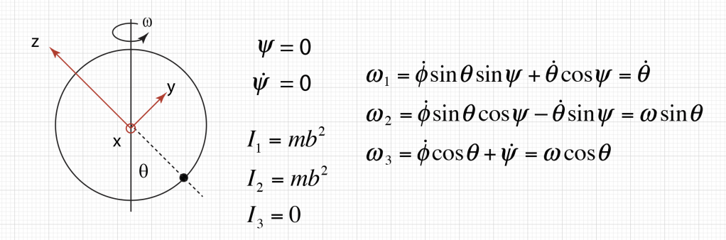
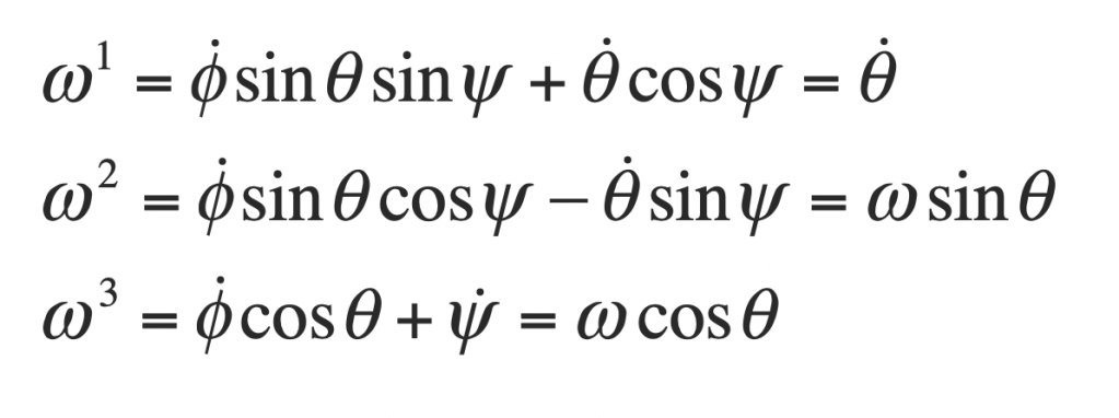
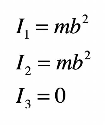
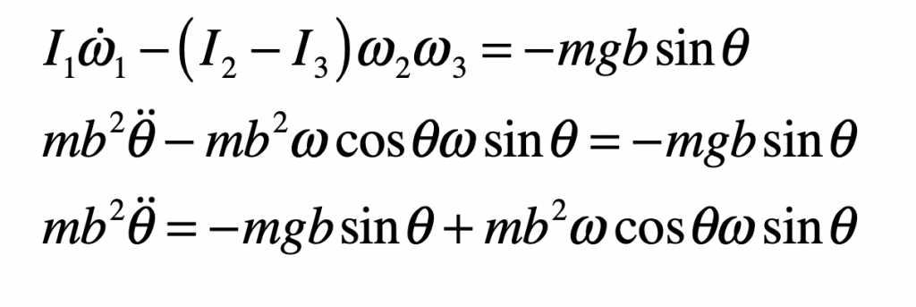
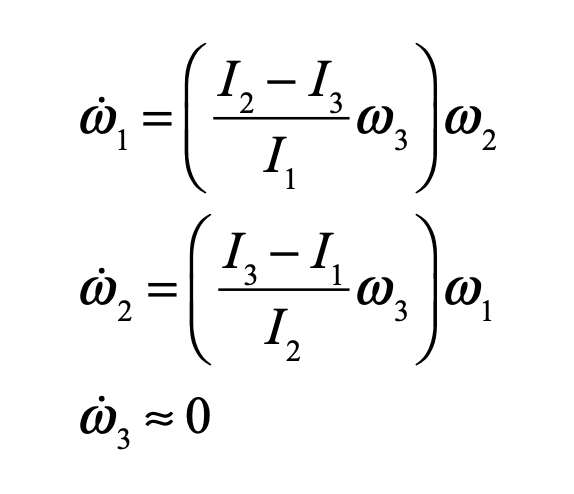
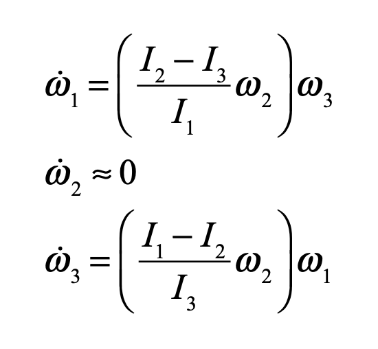
The flipping iPhone is a rigid body experiencing force-free motion. The Euler equations are an easy way to approach the somewhat complicated physics. These equations are

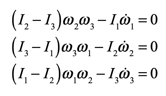
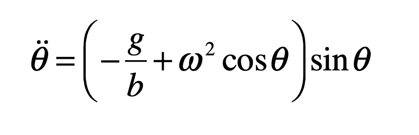
They all equal zero because there is no torque. First let’s assume the object is rotating mainly around the x1 axis so that ω2 and ω3 are small (rotating mainly around ω1).  Then solving for the angular accelerations yields

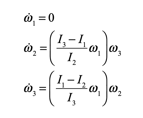
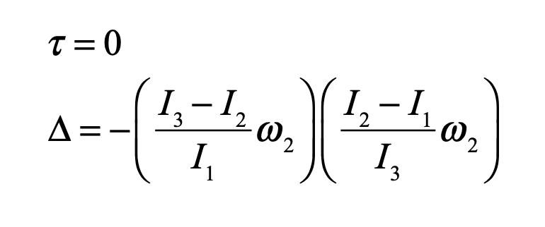
This is a two-dimensional flow equation in the variables  ω2, ω3.  Hence we can apply classic stability analysis for rotation mainly about the x1 axis. The Jacobian matrix is

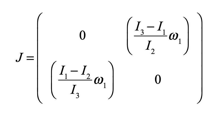
This matrix has a trace τ = 0 and a determinant Δ given by

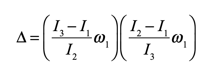
Because of the ordering I1 < I2 < I3 we know that this is quantity is positive. 

Armed with the trace and the determinant of a two-dimensional flow, we simply need to look at the 2D “stability space” as shown in Fig. 1. The horizontal axis is the determinant of the Jacobian matrix evaluated at the fixed point of the motion, and the vertical axis is the trace. In the case of the flipping iPhone, the Jacobian matrix is independent of both ω2 and ω3 (if they are remain small), so it has a global stability. When the determinant is positive, the stability depends on the trace. If the trace is positive, all motions are unstable (deviations grow exponentially). If the trace is negative, all motions are stable. The sideways parabola in the figure is known as the discriminant. If solutions are within the discriminant, they are spirals. As the trace approaches the origin, the spirals get slower and slow, until they become simple harmonic motions when the trace goes to zero. This kind of marginal stability is also known as centers. Centers have a stead-state stability without dissipation.

Fig. 1 The stability space for two-dimensional dynamics. The vertical axis is the trace of the Jacobian matrix and the horizontal axis is the determinant. If the determinant is negative, all motions are unstable saddle points. Otherwise, stability depends on the sign of the trace, unless the trace is zero, for which case the motion has steady-state stability like celestial orbits or harmonic oscillators. (Reprinted from Ref. [1])

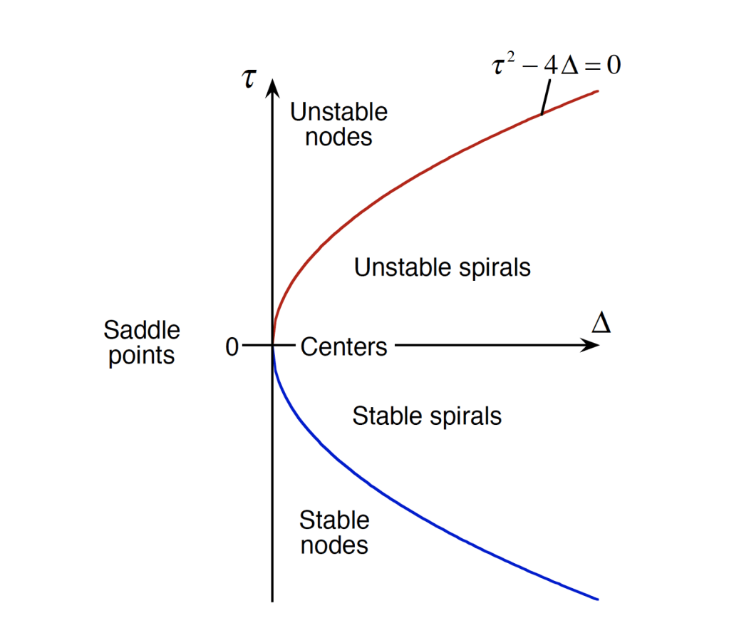
For the flipping iPhone (or tennis racket or book), the trace is zero and the determinant is positive for rotation mainly about the x1 axis, and the stability is therefore a “center”.  This is why the iPhone spins nicely about its axis with the smallest moment.

Let’s permute the indices to get the motion about the x3 axis with the largest moment. Then

The trace and determinant are

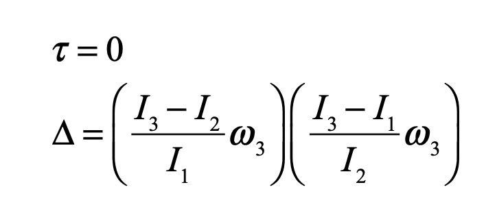
where the determinant is again positive and the stability is again a center.

But now let’s permute again so that the motion is mainly about the x2 axis with the intermediate moment.  In this case

And the trace and determinant are

The determinant is now negative, and from Fig. 1, this means that the stability is a saddle point. 

Saddle points in 2D have one stable manifold and one unstable manifold.  If the initial condition is just a little off the stability point, then the deviation will grow as the dynamical trajectory moves away from the equilibrium point along the unstable manifold.

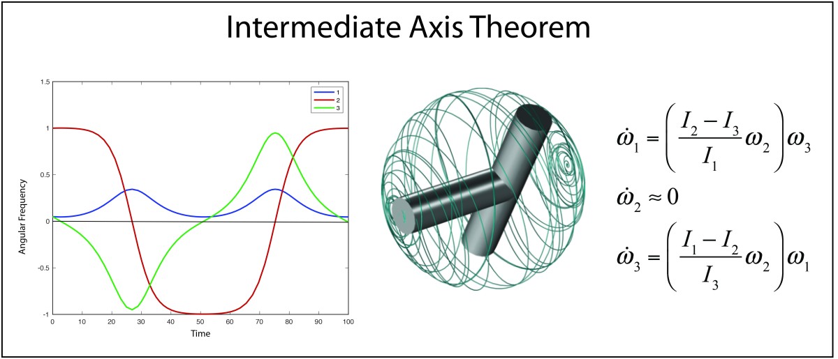
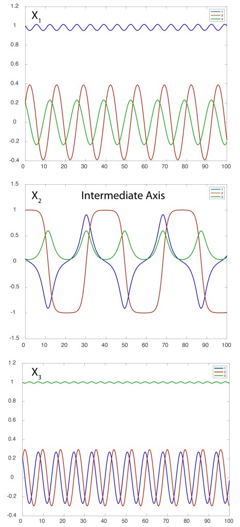
The components of the angular frequencies of each of these cases is shown in Fig. 2 for rotation mainly around x1, then x2 and then x3. A small amount of rotation is given as an initial condition about the other two axes for each case. For these calculations, no approximations were made, using the full Euler equations, and the motion is fully three-dimensional.

Fig. 2 Angular frequency components for motion with initial conditions of spin mainly about, respecitvely, the x1, x2 and x3 axes. The x2 case shows strong nonlinearity and slow unstable dynamics that periodically reverse. (I1 = 0.3, I2 = 0.5, I3 = 0.7)

Fate of the Spinning Earth

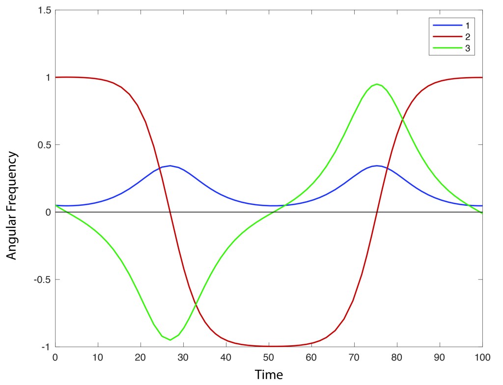
When two of the axes have very similar moments of inertia, that is, when the object becomes more symmetric, then the unstable dynamics can get very slow. An example is shown in Fig. 3 for I2 just a bit smaller than I3. The high frequency spin remains the same for long times and then quickly reverses. During the time when the spin is nearly stable, the other angular frequencies are close to zero, and the object would have only a slight wobble to it. Yet, in time, the wobble goes from bad to worse, until the whole thing flips over. It’s inevitable for almost any real-world solid…like maybe the Earth.

Fig. 3 Angular frequencies for a slightly asymmetric rigid body. The spin remains the same for long times and then flips suddenly.

The Earth is an oblate spheroid, wider at the equator because of the centrifugal force of the rotation. If it were a perfect spheroid, then the two moments orthogonal to the spin axis would be identically equal. However, the Earth has landmasses, continents, that make the moments of inertia slightly unequal. This would have catastrophic consequences, because if the Earth were perfectly rigid, then every few million years it should flip over, scrambling the seasons!

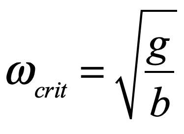
But that doesn’t happen. The reason is that the Earth has a liquid mantel and outer core that very slowly dissipate any wobble. The Earth, and virtually every celestial object that has any type of internal friction, always spins about its axis with the highest moment of inertia, which also means the system relaxes to its lowest kinetic energy for conserved L through the simple equation

So we are safe!

Python Code (FlipPhone.py)

Here is a simple Python code to explore the intermediate axis theorem. (Python code on GitHub.) Change the moments of inertia and change the initial conditions. Note that this program does not solve for the actual motions–the configuration-space trajectories. The solution of the Euler equations gives the time evolution of the three components of the angular velocity. Incremental rotations could be applied through rotation matrices operating on the configuration space to yield the configuration-space trajectory of the flipping iPhone (link to the technical details here).

#!/usr/bin/env python3
# -*- coding: utf-8 -*-
"""
Created on Thurs Oct 7 19:38:57 2021

@author: David Nolte
Introduction to Modern Dynamics, 2nd edition (Oxford University Press, 2019)

FlipPhone Example
"""
import numpy as np
import matplotlib as mpl
from mpl_toolkits.mplot3d import Axes3D
from scipy import integrate
from matplotlib import pyplot as plt

plt.close('all')
fig = plt.figure()
ax = fig.add_axes([0, 0, 1, 1], projection='3d')
ax.axis('on')

I1 = 0.45   # Moments of inertia can be changed here
I2 = 0.5
I3 = 0.55

def solve_lorenz(max_time=300.0):

# Flip Phone
    def flow_deriv(x_y_z, t0):

        x, y, z = x_y_z
        
        yp1 = ((I2-I3)/I1)*y*z;
        yp2 = ((I3-I1)/I2)*z*x;
        yp3 = ((I1-I2)/I3)*x*y;
        
        return [yp1, yp2, yp3]
    
    model_title = 'Flip Phone'

    t = np.linspace(0, max_time/4, int(250*max_time/4))

    # Solve for trajectories
    x0 = [[0.01,1,0.01]]   # Initial Conditions:  Change the major rotation axis here ....
    t = np.linspace(0, max_time, int(250*max_time))
    x_t = np.asarray([integrate.odeint(flow_deriv, x0i, t)
                      for x0i in x0])
     
    x, y, z = x_t[0,:,:].T
    lines = ax.plot(x, y, z, '-')
    plt.setp(lines, linewidth=0.5)

    ax.view_init(30, 30)
    plt.show()
    plt.title(model_title)
    plt.savefig('Flow3D')

    return t, x_t

ax.set_xlim((-1.1, 1.1))
ax.set_ylim((-1.1, 1.1))
ax.set_zlim((-1.1, 1.1))

t, x_t = solve_lorenz()

plt.figure(2)
lines = plt.plot(t,x_t[0,:,0],t,x_t[0,:,1],t,x_t[0,:,2])
plt.setp(lines, linewidth=1)


[1] D. D. Nolte, Introduction to Modern Dynamics, 2nd Edition (Oxford, 2019)

To see more on the Intermediate Axis Theorem, watch this amazing Youtube.

And here is another description of the Intermediate Axis Theorem.

Spontaneous Symmetry Breaking: A Mechanical Model

Symmetry is the canvas upon which the laws of physics are written. Symmetry defines the invariants of dynamical systems. But when symmetry breaks, the laws of physics break with it, sometimes in dramatic fashion. Take the Big Bang, for example, when a highly-symmetric form of the vacuum, known as the “false vacuum”, suddenly relaxed to a lower symmetry, creating an inflationary cascade of energy that burst forth as our Universe.

The early universe was extremely hot and energetic, so much so that all the forces of nature acted as one–described by a unified Lagrangian (as yet resisting discovery by theoretical physicists) of the highest symmetry. Yet as the universe expanded and cooled, the symmetry of the Lagrangian broke, and the unified forces split into two (gravity and electro-nuclear). As the universe cooled further, the Lagrangian (of the Standard Model) lost more symmetry as the electro-nuclear split into the strong nuclear force and the electro-weak force. Finally, at a tiny fraction of a second after the Big Bang, the universe cooled enough that the unified electro-week force broke into the electromagnetic force and the weak nuclear force. At each stage, spontaneous symmetry breaking occurred, and invariants of physics were broken, splitting into new behavior. In 2008, Yoichiro Nambu received the Nobel Prize in physics for his model of spontaneous symmetry breaking in subatomic physics.

Fig. 1 The spontanous symmetry breaking cascade after the Big Bang. From Ref.

Bifurcation Physics

Physics is filled with examples of spontaneous symmetry breaking. Crystallization and phase transitions are common examples. When the temperature is lowered on a fluid of molecules with high average local symmetry, the molecular interactions can suddenly impose lower-symmetry constraints on relative positions, and the liquid crystallizes into an ordered crystal. Even solid crystals can undergo a phase transition as one symmetry becomes energetically advantageous over another, and the crystal can change to a new symmetry.

In mechanics, any time a potential function evolves slowly with some parameter, it can start with one symmetry and evolve to another lower symmetry. The mechanical system governed by such a potential may undergo a discontinuous change in behavior.

In complex systems and chaos theory, sudden changes in behavior can be quite common as some parameter is changed continuously. These discontinuous changes in behavior, in response to a continuous change in a control parameter, is known as a bifurcation. There are many types of bifurcation, carrying descriptive names like the pitchfork bifurcation, period-doubling bifurcation, Hopf bifurcation, and fold bifurcation, among others. The pitchfork bifurcation is a typical example, shown in Fig. 2. As a parameter is changed continuously (horizontal axis), a stable fixed point suddenly becomes unstable and two new stable fixed points emerge at the same time. This type of bifurcation is called pitchfork because the diagram looks like a three-tined pitchfork. (This is technically called a supercritical pitchfork bifurcation. In a subcritical pitchfork bifurcation the solid and dashed lines are swapped.) This is exactly the bifurcation displayed by a simple mechanical model that illustrates spontaneous symmetry breaking.

Fig. 2 Bifurcation plot of a pitchfork bifurcation. As a parameter is changed smoothly and continuously (horizontal axis), a stable fixed point suddenly splits into three fixed points: one unstable and the other two stable.

Sliding Mass on a Rotating Hoop

One of the simplest mechanical models that displays spontaneous symmetry breaking and the pitchfork bifurcation is a bead sliding without friction on a circular hoop that is spinning on the vertical axis, as in Fig. 3. When it spins very slowly, this is just a simple pendulum with a stable equilibrium at the bottom, and it oscillates with a natural oscillation frequency ω0 = sqrt(g/b), where b is the radius of the hoop and g is the acceleration due to gravity. On the other hand, when it spins very fast, then the bead is flung to to one side or the other by centrifugal force. The bead then oscillates around one of the two new stable fixed points, but the fixed point at the bottom of the hoop is very unstable, because any deviation to one side or the other will cause the centrifugal force to kick in. (Note that in the body frame, centrifugal force is a non-inertial force that arises in the non-inertial coordinate frame. )

Fig. 3 A bead sliding without friction on a circular hoop rotating about a vertical axis. At high speed, the bead has a stable equilibrium to either side of the vertical.

The solution uses the Euler equations for the body frame along principal axes. In order to use the standard definitions of ω1, ω2, and ω3, the angle θ MUST be rotated around the x-axis.  This means the x-axis points out of the page in the diagram.  The y-axis is tilted up from horizontal by θ, and the z-axis is tilted from vertical by θ.  This establishes the body frame.

The components of the angular velocity are

And the moments of inertia are (assuming the bead is small)

There is only one Euler equation that is non-trivial. This is for the x-axis and the angle θ. The x-axis Euler equation is

and solving for the angular acceleration gives.

This is a harmonic oscillator with a “phase transition” that occurs as ω increases from zero.  At first the stable equilibrium is at the bottom.  But when ω passes a critical threshold, the equilibrium angle begins to increase to a finite angle set by the rotation speed.

This can only be real if  the magnitude of the argument is equal to or less than unity, which sets the critical threshold spin rate to make the system move to the new stable points to one side or the other for

which interestingly is the natural frequency of the non-rotating pendulum. Note that there are two equivalent angles (positive and negative), so this problem has a degeneracy. 

This is an example of a dynamical phase transition that leads to spontaneous symmetry breaking and a pitchfork bifurcation. By integrating the angular acceleration we can get the effective potential for the problem. One contribution to the potential is due to gravity. The other is centrifugal force. When combined and plotted in Fig. 4 for a family of values of the spin rate ω, a pitchfork emerges naturally by tracing the minima in the effective potential. The values of the new equilibrium angles are given in Fig. 2.

Fig. 4 Effective potential as a function of angle for a family of spin rates. At the transition spin rate, the effective potential is essentially flat with zero natural frequency. The pitchfork is the dashed green line.

Below the transition threshold for ω, the bottom of the hoop is the equilibrium position. To find the natural frequency of oscillation, expand the acceleration expression

For small oscillations the natural frequency is given by

As the effective potential gets flatter, the natural oscillation frequency decreases until it vanishes at the transition spin frequency. As the hoop spins even faster, the new equilibrium positions emerge. To find the natural frequency of the new equilibria, expand θ around the new equilibrium θ’ = θ – θ0

Which is a harmonic oscillator with oscillation angular frequency

Note that this is zero frequency at the transition threshold, then rises to match the spin rate of the hoop at high frequency. The natural oscillation frequency as a function of the spin looks like Fig. 5.

Fig. 5 Angular oscillation frequency for the bead. The bifurcation occurs at the critical spin rate ω = sqrt(g/b).

This mechanical analog is highly relevant for the spontaneous symmetry breaking that occurs in ferroelectric crystals when they go through a ferroelectric transition. At high temperature, these crystals have no internal polarization. But as the crystal cools towards the ferroelectric transition temperature, the optical-mode phonon modes “soften” as the phonon frequency decreases and vanishes at the transition temperature when the crystal spontaneously polarizes in one of several equivalent directions. The observation of mode softening in a polar crystal is one signature of an impending ferroelectric phase transition. Our mass on the hoop captures this qualitative physics nicely.

Golden Behavior

For fun, let’s find at what spin frequency the harmonic oscillation frequency at the dynamic equilibria equal the original natural frequency of the pendulum. Then

which is the golden ratio.  It’s spooky how often the golden ratio appears in random physics problems!