At the turn of the New Year, as I turn to the breakthroughs in physics of the previous year, sifting through the candidates, I usually narrow it down to about 4 to 6 that I find personally compelling (See, for instance 2023, 2022). In a given year, they may be related to things like supersolids, condensed atoms, or quantum entanglement. Often they relate to those awful, embarrassing gaps in physics knowledge that we give euphemistic names to, like “Dark Energy” and “Dark Matter” (although in the end they may be neither energy nor matter). But this year, as I sifted, I was struck by how many of the “physics” advances of the past year were focused on pushing limits—lower temperatures, more qubits, larger distances.
If you want something that is eventually useful, then engineering is the way to go, and many of the potential breakthroughs of 2024 did require heroic efforts. But if you are looking for a paradigm shift—a new way of seeing or thinking about our reality—then bigger, better and farther won’t give you that. We may be pushing the boundaries, but the thinking stays the same.
Therefore, for 2024, I have replaced “breakthrough” with a single “prospect” that may force us to change our thinking about the universe and the fundamental forces behind it.
This prospect is the weakening of dark energy over time.
It is a “prospect” because it is not yet absolutely confirmed. If it is confirmed in the next few years, then it changes our view of reality. If it is not confirmed, then it still forces us to think harder about fundamental questions, pointing where to look next.
Einstein’s Cosmological “Constant”
Like so much of physics today, the origins of this story go back to Einstein. At the height of WWI in 1917, as Einstein was working in Berlin, he “tweaked” his new theory of general relativity to allow the universe to be static. The tweak came in the form of a parameter he labelled Lambda (Λ), providing a counterbalance against the gravitational collapse of the universe, which at the time was assumed to have a time-invariant density. This cosmological “constant” of spacetime represented a pressure that kept the universe inflated like a balloon.
Fig. 1 Einstein’s “Field Equations” for the universe containing expressions for curvature, the metric tensor and energy density. Spacetime is warped by energy density, and trajectories within the warped spacetime follow geodesic curves. When Λ = 0, only gravitional attraction is present. When Λ ≠ 0, a “repulsive” background force exerts a pressure on spacetime, keeping it inflated like a balloon.
Later, in 1929 when Edwin Hubble discovered that the universe was not static but was expanding, and not only expanding, but apparently on a free trajectory originating at some point in the past (the Big Bang), Einstein zeroed out his cosmological constant, viewing it as one of his greatest blunders.
And so it stood until 1998 when two teams announced that the expansion of the universe is accelerating—and Einstein’s cosmological constant was back in. In addition, measurements of the energy density of the universe showed that the cosmological constant was contributing around 68% of the total energy density, which has been given the name of Dark Energy. One of the ways to measure Dark Energy is through BAO.
Baryon Acoustic Oscillations (BAO)
If the goal of science communication is to be transparent, and to engage the public in the heroic pursuit of pure science, then the moniker Baryon Acoustic Oscillations (BAO) was perhaps the wrong turn of phrase. “Cosmic Ripples” might have been a better analogy (and a bit more poetic).
In the early moments after the Big Bang, slight density fluctuations set up a balance of opposing effects between gravitational attraction, that tends to clump matter, and the homogenization effects of the hot photon background, that tends to disperse ionized matter. Matter consists of both dark matter as well as the matter we are composed of, known as baryonic matter. Only baryonic matter can be ionized and hence interact with photons, hence only photons and baryons experience this balance. As the universe expanded, an initial clump of baryons and photons expanded outward together, like the ripples on a millpond caused by a thrown pebble. And because the early universe had many clumps (and anti-clumps where density was lower than average), the millpond ripples were like those from a gentle rain with many expanding ringlets overlapping.
Fig. 2 Overlapping ripples showing galaxies formed along the shells. The size of the shells is set by the speed of “sound” in the universe. From [Ref].
Fig. 3 Left. Galaxies formed on acoustic ringlets like drops of dew on a spider’s web. Right. Many ringlets overlapping. The characteristic size of the ringlets can still be extracted statistically. From [Ref].
Then, about 400,000 years after the Big Bang, as the universe expanded and cooled, it got cold enough that ionized electrons and baryons formed atoms that are neutral and transparent to light. Light suddenly flew free, decoupled from the matter that had constrained it. Removing the balance between light and matter in the BAO caused the baryonic ripples to freeze in place, as if a sudden arctic blast froze the millpond in an instant. The residual clumps of matter in the early universe became clumps of galaxies in the modern universe that we can see and measure. We can also see the effects of those clumps on the temperature fluctuations of the cosmic microwave background (CMB).
Between these two—the BAO and the CMB—it is possible to measure cosmic distances, and with those distances, to measure how fast the universe is expanding.
Acceleration Slowing
The Dark Energy Spectroscopic Instrument (DESI) on top of Kitt Peak in Arizona is measuring the distances to millions of galaxies using automated fiber optic arrays containing thousands of optical fibers. In one year it measured the distances to about 6 milliion galaxies.
Fig. 4 The Kitt Peak observatory, the site of DESI. From [Ref].
By focusing on seven “epochs” in galaxy formation in the universe, it measures the sizes of the BAO ripples over time, ranging in ages from 3 billion to 11 billion years ago. (The universe is about 13.8 billion years old.) The relative sizes are then compared to the predictions of the LCDM (Lambda-Cold-Dark-Matter) model. This is the “consensus” model of the day—agreed upon as being “most likely” to explain observations. If Dark Energy is a true constant, then the relative sizes of the ripples should all be the same, regardless of how far back in time we look.
But what the DESI data discovered is that relative sizes more recently (a few billion years ago) are smaller than predicted by LCDM. Given that LCDM includes the acceleration of the expansion of the universe caused by Dark Energy, it means that Dark Energy is slightly weaker in the past few billion years than it was 10 billion years ago—it’s weakening or “thawing”.
The measurements as they stand today are shown in Fig. 5, showing the relative sizes as a function of how far back in time they look, with a dashed line showing the deviation from the LCDM prediction. The error bars in the figure are not yet are that impressive, and statistical effects may be causing the trend, so it might be erased by more measurements. But the BAO results have been augmented by recent measurements of supernova (SNe) that provide additional support for thawing Dark Energy. Combined, the BAO+SNe results currently stand at about 3.4 sigma. The gold standard for “discovery” is about 5 sigma, so there is still room for this effect to disappear. So stay tuned—the final answer may be known within a few years.
Fig. 5 Seven “epochs” in the evolution of galaxies in the universe. This plot shows relative galactic distances as a function of time looking back towards the Big Bang (older times closer to the Big Bang are to the right side of the graph). In more recent times, relative distances are smaller than predicted by the consensus theory known as Lambda-Cold-Dark-Matter (LCDM), suggesting that Dark Energy is slight weaker today than it was billions of years ago. The three left-most data points (with error bars from early 2024) are below the LCDM line. From [Ref].Fig. 6 Annotated version of the previous figure. From [Ref].
The Future of Physics
The gravitational constant G is considered to be a constant property of nature, as is Planck’s constant h, and the charge of the electron e. None of these fundamental properties of physics are viewed as time dependent and none can be derived from basic principles. They are simply constants of our reality. But if Λ is time dependent, then it is not a fundamental constant and should be derivable and explainable.
It may be hard to get excited about nothing … unless nothing is the whole ball game.
The only way we can really know what is, is by knowing what isn’t. Nothing is the backdrop against which we measure something. Experimentalists spend almost as much time doing control experiments, where nothing happens (or nothing is supposed to happen) as they spend measuring a phenomenon itself, the something.
Even the universe, full of so much something, came out of nothing during the Big Bang. And today the energy density of nothing, so-called Dark Energy, is blowing our universe apart, propelling it ever faster to a bitter cold end.
So here is a brief history of nothing, tracing how we have understood what it is, where it came from, and where is it today.
With sturdy shoulders, space stands opposing all its weight to nothingness. Where space is, there is being.
Friedrich Nietzsche
40,000 BCE – Cosmic Origins
This is a human history, about how we homo sapiens try to understand the natural world around us, so the first step on a history of nothing is the Big Bang of human consciousness that occurred sometime between 100,000 – 40,000 years ago. Some sort of collective phase transition happened in our thought process when we seem to have become aware of our own existence within the natural world. This time frame coincides with the beginning of representational art and ritual burial. This is also likely the time when human language skills reached their modern form, and when logical arguments–stories–first were told to explain our existence and origins.
Roughly two origin stories emerged from this time. One of these assumes that what is has always been, either continuously or cyclically. Buddhism and Hinduism are part of this tradition as are many of the origin philosophies of Indigenous North Americans. Another assumes that there was a beginning when everything came out of nothing. Abrahamic faiths (Let there be light!) subscribe to this creatio ex nihilo. What came before creation? Nothing!
500 BCE – Leucippus and Democritus Atomism
The Greek philosopher Leucippus and his student Democritus, living around 500 BCE, were the first to lay out the atomic theory in which the elements of substance were indivisible atoms of matter, and between the atoms of matter was void. The different materials around us were created by the different ways that these atoms collide and cluster together. Plato later adhered to this theory, developing ideas along these lines in his Timeaus.
300 BCE – Aristotle Vacuum
Aristotle is famous for arguing, in his Physics Book IV, Section 8, that nature abhors a vacuum (horror vacui) because any void would be immediately filled by the imposing matter surrounding it. He also argued more philosophically that nothing, by definition, cannot exist.
1644 – Rene Descartes Vortex Theory
Fast forward a millennia and a half, and theories of existence were finally achieving a level of sophistication that can be called “scientific”. Rene Descartes followed Aristotle’s views of the vacuum, but he extended it to the vacuum of space, filling it with an incompressible fluid in his Principles of Philosophy (1644). Just like water, laminar motion can only occur by shear, leading to vortices. Descartes was a better philosopher than mathematician, so it took Christian Huygens to apply mathematics to vortex motion to “explain” the gravitational effects of the solar system.
Otto von Guericke is one of those hidden gems of the history of science, a person who almost no-one remembers today, but who was far in advance of his own day. He was a powerful politician, holding the position of Burgomeister of the city of Magdeburg for more than 30 years, helping to rebuild it after it was sacked during the Thirty Years War. He was also a diplomat, playing a key role in the reorientation of power within the Holy Roman Empire. How he had free time is anyone’s guess, but he used it to pursue scientific interests that spanned from electrostatics to his invention of the vacuum pump.
With a succession of vacuum pumps, each better than the last, von Geuricke was like a kid in a toy factory, pumping the air out of anything he could find. In the process, he showed that a vacuum would extinguish a flame and could raise water in a tube.
His most famous demonstration was, of course, the Magdeburg sphere demonstration. In 1657 he fabricated two 20-inch hemispheres that he attached together with a vacuum seal and used his vacuum pump to evacuate the air from inside. He then attached chains from the hemispheres to a team of eight horses on each side, for a total of 16 horses, who were unable to separate the spheres. This dramatically demonstrated that air exerts a force on surfaces, and that Aristotle and Descartes were wrong—nature did allow a vacuum!
1667 – Isaac Newton Action at a Distance
When it came to the vacuum, Newton was agnostic. His universal theory of gravitation posited action at a distance, but the intervening medium played no direct role.
Nothing comes from nothing, Nothing ever could.
Rogers and Hammerstein, The Sound of Music
This would seem to say that Newton had nothing to say about the vacuum, but his other major work, his Optiks, established particles as the elements of light rays. Such light particles travelled easily through vacuum, so the particle theory of light came down on the empty side of space.
Statue of Isaac Newton by Sir Eduardo Paolozzi based on a painting by William Blake. Image Credit
1821 – Augustin Fresnel Luminiferous Aether
Today, we tend to think of Thomas Young as the chief proponent for the wave nature of light, going against the towering reputation of his own countryman Newton, and his courage and insights are admirable. But it was Augustin Fresnel who put mathematics to the theory. It was also Fresnel, working with his friend Francois Arago, who established that light waves are purely transverse.
For these contributions, Fresnel stands as one of the greatest physicists of the 1800’s. But his transverse light waves gave birth to one of the greatest red herrings of that century—the luminiferous aether. The argument went something like this, “if light is waves, then just as sound is oscillations of air, light must be oscillations of some medium that supports it – the luminiferous aether.” Arago searched for effects of this aether in his astronomical observations, but he didn’t see it, and Fresnel developed a theory of “partial aether drag” to account for Arago’s null measurement. Hippolyte Fizeau later confirmed the Fresnel “drag coefficient” in his famous measurement of the speed of light in moving water. (For the full story of Arago, Fresnel and Fizeau, see Chapter 2 of “Interference”. [1])
But the transverse character of light also required that this unknown medium must have some stiffness to it, like solids that support transverse elastic waves. This launched almost a century of alternative ideas of the aether that drew in such stellar actors as George Green, George Stokes and Augustin Cauchy with theories spanning from complete aether drag to zero aether drag with Fresnel’s partial aether drag somewhere in the middle.
1849 – Michael Faraday Field Theory
Micheal Faraday was one of the most intuitive physicists of the 1800’s. He worked by feel and mental images rather than by equations and proofs. He took nothing for granted, able to see what his experiments were telling him instead of looking only for what he expected.
This talent allowed him to see lines of force when he mapped out the magnetic field around a current-carrying wire. Physicists before him, including Ampere who developed a mathematical theory for the magnetic effects of a wire, thought only in terms of Newton’s action at a distance. All forces were central forces that acted in straight lines. Faraday’s experiments told him something different. The magnetic lines of force were circular, not straight. And they filled space. This realization led him to formulate his theory for the magnetic field.
Others at the time rejected this view, until William Thomson (the future Lord Kelvin) wrote a letter to Faraday in 1845 telling him that he had developed a mathematical theory for the field. He suggested that Faraday look for effects of fields on light, which Faraday found just one month later when he observed the rotation of the polarization of light when it propagated in a high-index material subject to a high magnetic field. This effect is now called Faraday Rotation and was one of the first experimental verifications of the direct effects of fields.
Nothing is more real than nothing.
Samuel Beckett
In 1949, Faraday stated his theory of fields in their strongest form, suggesting that fields in empty space were the repository of magnetic phenomena rather than magnets themselves [2]. He also proposed a theory of light in which the electric and magnetic fields induced each other in repeated succession without the need for a luminiferous aether.
1861 – James Clerk Maxwell Equations of Electromagnetism
James Clerk Maxwell pulled the various electric and magnetic phenomena together into a single grand theory, although the four succinct “Maxwell Equations” was condensed by Oliver Heaviside from Maxwell’s original 15 equations (written using Hamilton’s awkward quaternions) down to the 4 vector equations that we know and love today.
One of the most significant and most surprising thing to come out of Maxwell’s equations was the speed of electromagnetic waves that matched closely with the known speed of light, providing near certain proof that light was electromagnetic waves.
However, the propagation of electromagnetic waves in Maxwell’s theory did not rule out the existence of a supporting medium—the luminiferous aether. It was still not clear that fields could exist in a pure vacuum but might still be like the stress fields in solids.
Late in his life, just before he died, Maxwell pointed out that no measurement of relative speed through the aether performed on a moving Earth could see deviations that were linear in the speed of the Earth but instead would be second order. He considered that such second-order effects would be far to small ever to detect, but Albert Michelson had different ideas.
1887 – Albert Michelson Null Experiment
Albert Michelson was convinced of the existence of the luminiferous aether, and he was equally convinced that he could detect it. In 1880, working in the basement of the Potsdam Observatory outside Berlin, he operated his first interferometer in a search for evidence of the motion of the Earth through the aether. He had built the interferometer, what has come to be called a Michelson Interferometer, months earlier in the laboratory of Hermann von Helmholtz in the center of Berlin, but the footfalls of the horse carriages outside the building disturbed the measurements too much—Postdam was quieter.
But he could find no difference in his interference fringes as he oriented the arms of his interferometer parallel and orthogonal to the Earth’s motion. A simple calculation told him that his interferometer design should have been able to detect it—just barely—so the null experiment was a puzzle.
Seven years later, again in a basement (this time in a student dormitory at Western Reserve College in Cleveland, Ohio), Michelson repeated the experiment with an interferometer that was ten times more sensitive. He did this in collaboration with Edward Morley. But again, the results were null. There was no difference in the interference fringes regardless of which way he oriented his interferometer. Motion through the aether was undetectable.
(Michelson has a fascinating backstory, complete with firestorms (literally) and the Wild West and a moment when he was almost committed to an insane asylum against his will by a vengeful wife. To read all about this, see Chapter 4: After the Gold Rush in my recent book Interference (Oxford, 2023)).
The Michelson Morley experiment did not create the crisis in physics that it is sometimes credited with. They published their results, and the physics world took it in stride. Voigt and Fitzgerald and Lorentz and Poincaré toyed with various ideas to explain it away, but there had already been so many different models, from complete drag to no drag, that a few more theories just added to the bunch.
But they all had their heads in a haze. It took an unknown patent clerk in Switzerland to blow away the wisps and bring the problem into the crystal clear.
1905 – Albert Einstein Relativity
So much has been written about Albert Einstein’s “miracle year” of 1905 that it has lapsed into a form of physics mythology. Looking back, it seems like his own personal Big Bang, springing forth out of the vacuum. He published 5 papers that year, each one launching a new approach to physics on a bewildering breadth of problems from statistical mechanics to quantum physics, from electromagnetism to light … and of course, Special Relativity [3].
Whereas the others, Voigt and Fitzgerald and Lorentz and Poincaré, were trying to reconcile measurements of the speed of light in relative motion, Einstein just replaced all that musing with a simple postulate, his second postulate of relativity theory:
2. Any ray of light moves in the “stationary” system of co-ordinates with the determined velocity c, whether the ray be emitted by a stationary or by a moving body. Hence …
Albert Einstein, Annalen der Physik, 1905
And the rest was just simple algebra—in complete agreement with Michelson’s null experiment, and with Fizeau’s measurement of the so-called Fresnel drag coefficient, while also leading to the famous E = mc2 and beyond.
There is no aether. Electromagnetic waves are self-supporting in vacuum—changing electric fields induce changing magnetic fields that induce, in turn, changing electric fields—and so it goes.
The vacuum is vacuum—nothing! Except that it isn’t. It is still full of things.
1931 – P. A. M Dirac Antimatter
The Dirac equation is the famous end-product of P. A. M. Dirac’s search for a relativistic form of the Schrödinger equation. It replaces the asymmetric use in Schrödinger’s form of a second spatial derivative and a first time derivative with Dirac’s form using only first derivatives that are compatible with relativistic transformations [4].
One of the immediate consequences of this equation is a solution that has negative energy. At first puzzling and hard to interpret [5], Dirac eventually hit on the amazing proposal that these negative energy states are real particles paired with ordinary particles. For instance, the negative energy state associated with the electron was an anti-electron, a particle with the same mass as the electron, but with positive charge. Furthermore, because the anti-electron has negative energy and the electron has positive energy, these two particles can annihilate and convert their mass energy into the energy of gamma rays. This audacious proposal was confirmed by the American physicist Carl Anderson who discovered the positron in 1932.
The existence of particles and anti-particles, combined with Heisenberg’s uncertainty principle, suggests that vacuum fluctuations can spontaneously produce electron-positron pairs that would then annihilate within a time related to the mass energy
Although this is an exceedingly short time (about 10-21 seconds), it means that the vacuum is not empty, but contains a frothing sea of particle-antiparticle pairs popping into and out of existence.
1938 – M. C. Escher Negative Space
Scientists are not the only ones who think about empty space. Artists, too, are deeply committed to a visual understanding of our world around us, and the uses of negative space in art dates back virtually to the first cave paintings. However, artists and art historians only talked explicitly in such terms since the 1930’s and 1940’s [6]. One of the best early examples of the interplay between positive and negative space was a print made by M. C. Escher in 1938 titled “Day and Night”.
1946 – Edward Purcell Modified Spontaneous Emission
In 1916 Einstein laid out the laws of photon emission and absorption using very simple arguments (his modus operandi) based on the principles of detailed balance. He discovered that light can be emitted either spontaneously or through stimulated emission (the basis of the laser) [7]. Once the nature of vacuum fluctuations was realized through the work of Dirac, spontaneous emission was understood more deeply as a form of stimulated emission caused by vacuum fluctuations. In the absence of vacuum fluctuations, spontaneous emission would be inhibited. Conversely, if vacuum fluctuations are enhanced, then spontaneous emission would be enhanced.
This effect was observed by Edward Purcell in 1946 through the observation of emission times of an atom in a RF cavity [8]. When the atomic transition was resonant with the cavity, spontaneous emission times were much faster. The Purcell enhancement factor is
where Q is the “Q” of the cavity, and V is the cavity volume. The physical basis of this effect is the modification of vacuum fluctuations by the cavity modes caused by interference effects. When cavity modes have constructive interference, then vacuum fluctuations are larger, and spontaneous emission is stimulated more quickly.
1948 – Hendrik Casimir Vacuum Force
Interference effects in a cavity affect the total energy of the system by excluding some modes which become inaccessible to vacuum fluctuations. This lowers the internal energy internal to a cavity relative to free space outside the cavity, resulting in a net “pressure” acting on the cavity. If two parallel plates are placed in close proximity, this would cause a force of attraction between them. The effect was predicted in 1948 by Hendrik Casimir [9], but it was not verified experimentally until 1997 by S. Lamoreaux at Yale University [10].
Two plates brought very close feel a pressure exerted by the higher vacuum energy density external to the cavity.
1949 – Shinichiro Tomonaga, Richard Feynman and Julian Schwinger QED
The physics of the vacuum in the years up to 1948 had been a hodge-podge of ad hoc theories that captured the qualitative aspects, and even some of the quantitative aspects of vacuum fluctuations, but a consistent theory was lacking until the work of Tomonaga in Japan, Feynman at Cornell and Schwinger at Harvard. Feynman and Schwinger both published their theory of quantum electrodynamics (QED) in 1949. They were actually scooped by Tomonaga, who had developed his theory earlier during WWII, but physics research in Japan had been cut off from the outside world. It was when Oppenheimer received a letter from Tomonaga in 1949 that the West became aware of his work. All three received the Nobel Prize for their work on QED in 1965. Precision tests of QED now make it one of the most accurately confirmed theories in physics.
Richard Feynman’s first “Feynman diagram”.
1964 – Peter Higgs and The Higgs
The Higgs particle, known as “The Higgs”, was the brain-child of Peter Higgs, Francois Englert and Gerald Guralnik in 1964. Higgs’ name became associated with the theory because of a response letter he wrote to an objection made about the theory. The Higg’s mechanism is spontaneous symmetry breaking in which a high-symmetry potential can lower its energy by distorting the field, arriving at a new minimum in the potential. This mechanism can allow the bosons that carry force to acquire mass (something the earlier Yang-Mills theory could not do).
Spontaneous symmetry breaking is a ubiquitous phenomenon in physics. It occurs in the solid state when crystals can lower their total energy by slightly distorting from a high symmetry to a low symmetry. It occurs in superconductors in the formation of Cooper pairs that carry supercurrents. And here it occurs in the Higgs field as the mechanism to imbues particles with mass .
Conceptual graph of a potential surface where the high symmetry potential is higher than when space is distorted to lower symmetry. Image Credit
The theory was mostly ignored for its first decade, but later became the core of theories of electroweak unification. The Large Hadron Collider (LHC) at Geneva was built to detect the boson, announced in 2012. Peter Higgs and Francois Englert were awarded the Nobel Prize in Physics in 2013, just one year after the discovery.
The Higgs field permeates all space, and distortions in this field around idealized massless point particles are observed as mass. In this way empty space becomes anything but.
1981 – Alan Guth Inflationary Big Bang
Problems arose in observational cosmology in the 1970’s when it was understood that parts of the observable universe that should have been causally disconnected were in thermal equilibrium. This could only be possible if the universe were much smaller near the very beginning. In January of 1981, Alan Guth, then at Cornell University, realized that a rapid expansion from an initial quantum fluctuation could be achieved if an initial “false vacuum” existed in a positive energy density state (negative vacuum pressure). Such a false vacuum could relax to the ordinary vacuum, causing a period of very rapid growth that Guth called “inflation”. Equilibrium would have been achieved prior to inflation, solving the observational problem.Therefore, the inflationary model posits a multiplicities of different types of “vacuum”, and once again, simple vacuum is not so simple.
Energy density as a function of a scalar variable. Quantum fluctuations create a “false vacuum” that can relax to “normal vacuum: by expanding rapidly. Image Credit
1998 – Saul Pearlmutter Dark Energy
Einstein didn’t make many mistakes, but in the early days of General Relativity he constructed a theoretical model of a “static” universe. A central parameter in Einstein’s model was something called the Cosmological Constant. By tuning it to balance gravitational collapse, he tuned the universe into a static Ithough unstable) state. But when Edwin Hubble showed that the universe was expanding, Einstein was proven incorrect. His Cosmological Constant was set to zero and was considered to be a rare blunder.
Fast forward to 1999, and the Supernova Cosmology Project, directed by Saul Pearlmutter, discovered that the expansion of the universe was accelerating. The simplest explanation was that Einstein had been right all along, or at least partially right, in that there was a non-zero Cosmological Constant. Not only is the universe not static, but it is literally blowing up. The physical origin of the Cosmological Constant is believed to be a form of energy density associated with the space of the universe. This “extra” energy density has been called “Dark Energy”, filling empty space.
The bottom line is that nothing, i.e., the vacuum, is far from nothing. It is filled with a froth of particles, and energy, and fields, and potentials, and broken symmetries, and negative pressures, and who knows what else as modern physics has been much ado about this so-called nothing, almost more than it has been about everything else.
[2] L. Peirce Williams in “Faraday, Michael.” Complete Dictionary of Scientific Biography, vol. 4, Charles Scribner’s Sons, 2008, pp. 527-540.
[3] A. Einstein, “On the electrodynamics of moving bodies,” Annalen Der Physik 17, 891-921 (1905).
[4] Dirac, P. A. M. (1928). “The Quantum Theory of the Electron”. Proceedings of the Royal Society A: Mathematical, Physical and Engineering Sciences. 117 (778): 610–624.
[5] Dirac, P. A. M. (1930). “A Theory of Electrons and Protons”. Proceedings of the Royal Society A: Mathematical, Physical and Engineering Sciences. 126 (801): 360–365.
[6] Nikolai M Kasak, Physical Art: Action of positive and negative space, (Rome, 1947/48) [2d part rev. in 1955 and 1956].
[7] A. Einstein, “Strahlungs-Emission un -Absorption nach der Quantentheorie,” Verh. Deutsch. Phys. Ges. 18, 318 (1916).
[8] Purcell, E. M. (1946-06-01). “Proceedings of the American Physical Society: Spontaneous Emission Probabilities at Ratio Frequencies”. Physical Review. American Physical Society (APS). 69 (11–12): 681.
[9] Casimir, H. B. G. (1948). “On the attraction between two perfectly conducting plates”. Proc. Kon. Ned. Akad. Wet. 51: 793.
[10] Lamoreaux, S. K. (1997). “Demonstration of the Casimir Force in the 0.6 to 6 μm Range”. Physical Review Letters. 78 (1): 5–8.
Read more in Books by David Nolte at Oxford University Press
If you are a fan of the Doppler effect, then time trials at the Indy 500 Speedway will floor you. Even if you have experienced the fall in pitch of a passing train whistle while stopped in your car at a railroad crossing, or heard the falling whine of a jet passing overhead, I can guarantee that you have never heard anything like an Indy car passing you by at 225 miles an hour.
Indy 500 Time Trials and the Doppler Effect
The Indy 500 time trials are the best way to experience the effect, rather than on race day when there is so much crowd noise and the overlapping sounds of all the cars. During the week before the race, the cars go out on the track, one by one, in time trials to decide the starting order in the pack on race day. Fans are allowed to wander around the entire complex, so you can get right up to the fence at track level on the straight-away. The cars go by only thirty feet away, so they are coming almost straight at you as they approach and straight away from you as they leave. The whine of the car as it approaches is 43% higher than when it is standing still, and it drops to 33% lower than the standing frequency—a ratio almost approaching a factor of two. And they go past so fast, it is almost a step function, going from a steady high note to a steady low note in less than a second. That is the Doppler effect!
But as obvious as the acoustic Doppler effect is to us today, it was far from obvious when it was proposed in 1842 by Christian Doppler at a time when trains, the fastest mode of transport at the time, ran at 20 miles per hour or less. In fact, Doppler’s theory generated so much controversy that the Academy of Sciences of Vienna held a trial in 1853 to decide its merit—and Doppler lost! For the surprising story of Doppler and the fate of his discovery, see my Physics Today article.
From that fraught beginning, the effect has expanded in such importance, that today it is a daily part of our lives. From Doppler weather radar, to speed traps on the highway, to ultrasound images of babies—Doppler is everywhere.
Development of the Doppler-Fizeau Effect
When Doppler proposed the shift in color of the light from stars in 1842 [1], depending on their motion towards or away from us, he may have been inspired by his walk to work every morning, watching the ripples on the surface of the Vltava River in Prague as the water slipped by the bridge piers. The drawings in his early papers look reminiscently like the patterns you see with compressed ripples on the upstream side of the pier and stretched out on the downstream side. Taking this principle to the night sky, Doppler envisioned that binary stars, where one companion was blue and the other was red, was caused by their relative motion. He could not have known at that time that typical binary star speeds were too small to cause this effect, but his principle was far more general, applying to all wave phenomena.
Six years later in 1848 [2], the French physicist Armand Hippolyte Fizeau, soon to be famous for making the first direct measurement of the speed of light, proposed the same principle, unaware of Doppler’s publications in German. As Fizeau was preparing his famous measurement, he originally worked with a spinning mirror (he would ultimately use a toothed wheel instead) and was thinking about what effect the moving mirror might have on the reflected light. He considered the effect of star motion on starlight, just as Doppler had, but realized that it was more likely that the speed of the star would affect the locations of the spectral lines rather than change the color. This is in fact the correct argument, because a Doppler shift on the black-body spectrum of a white or yellow star shifts a bit of the infrared into the visible red portion, while shifting a bit of the ultraviolet out of the visible, so that the overall color of the star remains the same, but Fraunhofer lines would shift in the process. Because of the independent development of the phenomenon by both Doppler and Fizeau, and because Fizeau was a bit clearer in the consequences, the effect is more accurately called the Doppler-Fizeau Effect, and in France sometimes only as the Fizeau Effect. Here in the US, we tend to forget the contributions of Fizeau, and it is all Doppler.
Fig. 1 The title page of Doppler’s 1842 paper [1] proposing the shift in color of stars caused by their motions. (“On the colored light of double stars and a few other stars in the heavens: Study of an integral part of Bradley’s general aberration theory”)
Fig. 2 Doppler used simple proportionality and relative velocities to deduce the first-order change in frequency of waves caused by motion of the source relative to the receiver, or of the receiver relative to the source.
Fig. 3 Doppler’s drawing of what would later be called the Mach cone generating a shock wave. Mach was one of Doppler’s later champions, making dramatic laboratory demonstrations of the acoustic effect, even as skepticism persisted in accepting the phenomenon.
Doppler and Exoplanet Discovery
It is fitting that many of today’s applications of the Doppler effect are in astronomy. His original idea on binary star colors was wrong, but his idea that relative motion changes frequencies was right, and it has become one of the most powerful astrometric techniques in astronomy today. One of its important recent applications was in the discovery of extrasolar planets orbiting distant stars.
When a large planet like Jupiter orbits a star, the center of mass of the two-body system remains at a constant point, but the individual centers of mass of the planet and the star both orbit the common point. This makes it look like the star has a wobble, first moving towards our viewpoint on Earth, then moving away. Because of this relative motion of the star, the light can appear blueshifted caused by the Doppler effect, then redshifted with a set periodicity. This was observed by Queloz and Mayer in 1995 for the star 51 Pegasi, which represented the first detection of an exoplanet [3]. The duo won the Nobel Prize in 2019 for the discovery.
Fig. 4 A gas giant (like Jupiter) and a star obit a common center of mass causing the star to wobble. The light of the star when viewed at Earth is periodically red- and blue-shifted by the Doppler effect. From Ref.
Doppler and Vera Rubins’ Galaxy Velocity Curves
In the late 1960’s and early 1970’s Vera Rubin at the Carnegie Institution of Washington used newly developed spectrographs to use the Doppler effect to study the speeds of ionized hydrogen gas surrounding massive stars in individual galaxies [4]. From simple Newtonian dynamics it is well understood that the speed of stars as a function of distance from the galactic center should increase with increasing distance up to the average radius of the galaxy, and then should decrease at larger distances. This trend in speed as a function of radius is called a rotation curve. As Rubin constructed the rotation curves for many galaxies, the increase of speed with increasing radius at small radii emerged as a clear trend, but the stars farther out in the galaxies were all moving far too fast. In fact, they are moving so fast that they exceeded escape velocity and should have flown off into space long ago. This disturbing pattern was repeated consistently in one rotation curve after another for many galaxies.
Fig. 5 Locations of Doppler shifts of ionized hydrogen measured by Vera Rubin on the Andromeda galaxy. From Ref.
Fig. 6 Vera Rubin’s velocity curve for the Andromeda galaxy. From Ref.
Fig. 7 Measured velocity curves relative to what is expected from the visible mass distribution of the galaxy. From Ref.
A simple fix to the problem of the rotation curves is to assume that there is significant mass present in every galaxy that is not observable either as luminous matter or as interstellar dust. In other words, there is unobserved matter, dark matter, in all galaxies that keeps all their stars gravitationally bound. Estimates of the amount of dark matter needed to fix the velocity curves is about five times as much dark matter as observable matter. In short, 80% of the mass of a galaxy is not normal. It is neither a perturbation nor an artifact, but something fundamental and large. The discovery of the rotation curve anomaly by Rubin using the Doppler effect stands as one of the strongest evidence for the existence of dark matter.
There is so much dark matter in the Universe that it must have a major effect on the overall curvature of space-time according to Einstein’s field equations. One of the best probes of the large-scale structure of the Universe is the afterglow of the Big Bang, known as the cosmic microwave background (CMB).
Doppler and the Big Bang
The Big Bang was astronomically hot, but as the Universe expanded it cooled. About 380,000 years after the Big Bang, the Universe cooled sufficiently that the electron-proton plasma that filled space at that time condensed into hydrogen. Plasma is charged and opaque to photons, while hydrogen is neutral and transparent. Therefore, when the hydrogen condensed, the thermal photons suddenly flew free and have continued unimpeded, continuing to cool. Today the thermal glow has reached about three degrees above absolute zero. Photons in thermal equilibrium with this low temperature have an average wavelength of a few millimeters corresponding to microwave frequencies, which is why the afterglow of the Big Bang got its name: the Cosmic Microwave Background (CMB).
Not surprisingly, the CMB has no preferred reference frame, because every point in space is expanding relative to every other point in space. In other words, space itself is expanding. Yet soon after the CMB was discovered by Arno Penzias and Robert Wilson (for which they were awarded the Nobel Prize in Physics in 1978), an anisotropy was discovered in the background that had a dipole symmetry caused by the Doppler effect as the Solar System moves at 368±2 km/sec relative to the rest frame of the CMB. Our direction is towards galactic longitude 263.85o and latitude 48.25o, or a bit southwest of Virgo. Interestingly, the local group of about 100 galaxies, of which the Milky Way and Andromeda are the largest members, is moving at 627±22 km/sec in the direction of galactic longitude 276o and latitude 30o. Therefore, it seems like we are a bit slack in our speed compared to the rest of the local group. This is in part because we are being pulled towards Andromeda in roughly the opposite direction, but also because of the speed of the solar system in our Galaxy.
Fig. 8 The CMB dipole anisotropy caused by the Doppler effect as the Earth moves at 368 km/sec through the rest frame of the CMB.
Aside from the dipole anisotropy, the CMB is amazingly uniform when viewed from any direction in space, but not perfectly uniform. At the level of 0.005 percent, there are variations in the temperature depending on the location on the sky. These fluctuations in background temperature are called the CMB anisotropy, and they help interpret current models of the Universe. For instance, the average angular size of the fluctuations is related to the overall curvature of the Universe. This is because, in the early Universe, not all parts of it were in communication with each other. This set an original spatial size to thermal discrepancies. As the Universe continued to expand, the size of the regional variations expanded with it, and the sizes observed today would appear larger or smaller, depending on how the universe is curved. Therefore, to measure the energy density of the Universe, and hence to find its curvature, required measurements of the CMB temperature that were accurate to better than a part in 10,000.
Equivalently, parts of the early universe had greater mass density than others, causing the gravitational infall of matter towards these regions. Then, through the Doppler effect, light emitted (or scattered) by matter moving towards these regions contributes to the anisotropy. They contribute what are known as “Doppler peaks” in the spatial frequency spectrum of the CMB anisotropy.
Fig. 9 The CMB small-scale anisotropy, part of which is contributed by Doppler shifts of matter falling into denser regions in the early universe.
The examples discussed in this blog (exoplanet discovery, galaxy rotation curves, and cosmic background) are just a small sampling of the many ways that the Doppler effect is used in Astronomy. But clearly, Doppler has played a key role in the long history of the universe.
By David D. Nolte, Jan. 23, 2022
References:
[1] C. A. DOPPLER, “Über das farbige Licht der Doppelsterne und einiger anderer Gestirne des Himmels (About the coloured light of the binary stars and some other stars of the heavens),” Proceedings of the Royal Bohemian Society of Sciences, vol. V, no. 2, pp. 465–482, (Reissued 1903) (1842)
[2] H. Fizeau, “Acoustique et optique,” presented at the Société Philomathique de Paris, Paris, 1848.
[3] M. Mayor and D. Queloz, “A JUPITER-MASS COMPANION TO A SOLAR-TYPE STAR,” Nature, vol. 378, no. 6555, pp. 355-359, Nov (1995)
[4] Rubin, Vera; Ford, Jr., W. Kent (1970). “Rotation of the Andromeda Nebula from a Spectroscopic Survey of Emission Regions”. The Astrophysical Journal. 159: 379
M. Tegmark, “Doppler peaks and all that: CMB anisotropies and what they can tell us,” in International School of Physics Enrico Fermi Course 132 on Dark Matter in the Universe, Varenna, Italy, Jul 25-Aug 04 1995, vol. 132, in Proceedings of the International School of Physics Enrico Fermi, 1996, pp. 379-416
Symmetry is the canvas upon which the laws of physics are written. Symmetry defines the invariants of dynamical systems. But when symmetry breaks, the laws of physics break with it, sometimes in dramatic fashion. Take the Big Bang, for example, when a highly-symmetric form of the vacuum, known as the “false vacuum”, suddenly relaxed to a lower symmetry, creating an inflationary cascade of energy that burst forth as our Universe.
The early universe was extremely hot and energetic, so much so that all the forces of nature acted as one–described by a unified Lagrangian (as yet resisting discovery by theoretical physicists) of the highest symmetry. Yet as the universe expanded and cooled, the symmetry of the Lagrangian broke, and the unified forces split into two (gravity and electro-nuclear). As the universe cooled further, the Lagrangian (of the Standard Model) lost more symmetry as the electro-nuclear split into the strong nuclear force and the electro-weak force. Finally, at a tiny fraction of a second after the Big Bang, the universe cooled enough that the unified electro-week force broke into the electromagnetic force and the weak nuclear force. At each stage, spontaneous symmetry breaking occurred, and invariants of physics were broken, splitting into new behavior. In 2008, Yoichiro Nambu received the Nobel Prize in physics for his model of spontaneous symmetry breaking in subatomic physics.
Fig. 1 The spontanous symmetry breaking cascade after the Big Bang. From Ref.
Bifurcation Physics
Physics is filled with examples of spontaneous symmetry breaking. Crystallization and phase transitions are common examples. When the temperature is lowered on a fluid of molecules with high average local symmetry, the molecular interactions can suddenly impose lower-symmetry constraints on relative positions, and the liquid crystallizes into an ordered crystal. Even solid crystals can undergo a phase transition as one symmetry becomes energetically advantageous over another, and the crystal can change to a new symmetry.
In mechanics, any time a potential function evolves slowly with some parameter, it can start with one symmetry and evolve to another lower symmetry. The mechanical system governed by such a potential may undergo a discontinuous change in behavior.
In complex systems and chaos theory, sudden changes in behavior can be quite common as some parameter is changed continuously. These discontinuous changes in behavior, in response to a continuous change in a control parameter, is known as a bifurcation. There are many types of bifurcation, carrying descriptive names like the pitchfork bifurcation, period-doubling bifurcation, Hopf bifurcation, and fold bifurcation, among others. The pitchfork bifurcation is a typical example, shown in Fig. 2. As a parameter is changed continuously (horizontal axis), a stable fixed point suddenly becomes unstable and two new stable fixed points emerge at the same time. This type of bifurcation is called pitchfork because the diagram looks like a three-tined pitchfork. (This is technically called a supercritical pitchfork bifurcation. In a subcritical pitchfork bifurcation the solid and dashed lines are swapped.) This is exactly the bifurcation displayed by a simple mechanical model that illustrates spontaneous symmetry breaking.
Fig. 2 Bifurcation plot of a pitchfork bifurcation. As a parameter is changed smoothly and continuously (horizontal axis), a stable fixed point suddenly splits into three fixed points: one unstable and the other two stable.
Sliding Mass on a Rotating Hoop
One of the simplest mechanical models that displays spontaneous symmetry breaking and the pitchfork bifurcation is a bead sliding without friction on a circular hoop that is spinning on the vertical axis, as in Fig. 3. When it spins very slowly, this is just a simple pendulum with a stable equilibrium at the bottom, and it oscillates with a natural oscillation frequency ω0 = sqrt(g/b), where b is the radius of the hoop and g is the acceleration due to gravity. On the other hand, when it spins very fast, then the bead is flung to to one side or the other by centrifugal force. The bead then oscillates around one of the two new stable fixed points, but the fixed point at the bottom of the hoop is very unstable, because any deviation to one side or the other will cause the centrifugal force to kick in. (Note that in the body frame, centrifugal force is a non-inertial force that arises in the non-inertial coordinate frame. )
Fig. 3 A bead sliding without friction on a circular hoop rotating about a vertical axis. At high speed, the bead has a stable equilibrium to either side of the vertical.
The solution uses the Euler equations for the body frame along principal axes. In order to use the standard definitions of ω1, ω2, and ω3, the angle θ MUST be rotated around the x-axis. This means the x-axis points out of the page in the diagram. The y-axis is tilted up from horizontal by θ, and the z-axis is tilted from vertical by θ. This establishes the body frame.
The components of the angular velocity are
And the moments of inertia are (assuming the bead is small)
There is only one Euler equation that is non-trivial. This is for the x-axis and the angle θ. The x-axis Euler equation is
and solving for the angular acceleration gives.
This is a harmonic oscillator with a “phase transition” that occurs as ω increases from zero. At first the stable equilibrium is at the bottom. But when ω passes a critical threshold, the equilibrium angle begins to increase to a finite angle set by the rotation speed.
This can only be real if the magnitude of the argument is equal to or less than unity, which sets the critical threshold spin rate to make the system move to the new stable points to one side or the other for
which interestingly is the natural frequency of the non-rotating pendulum. Note that there are two equivalent angles (positive and negative), so this problem has a degeneracy.
This is an example of a dynamical phase transition that leads to spontaneous symmetry breaking and a pitchfork bifurcation. By integrating the angular acceleration we can get the effective potential for the problem. One contribution to the potential is due to gravity. The other is centrifugal force. When combined and plotted in Fig. 4 for a family of values of the spin rate ω, a pitchfork emerges naturally by tracing the minima in the effective potential. The values of the new equilibrium angles are given in Fig. 2.
Fig. 4 Effective potential as a function of angle for a family of spin rates. At the transition spin rate, the effective potential is essentially flat with zero natural frequency. The pitchfork is the dashed green line.
Below the transition threshold for ω, the bottom of the hoop is the equilibrium position. To find the natural frequency of oscillation, expand the acceleration expression
For small oscillations the natural frequency is given by
As the effective potential gets flatter, the natural oscillation frequency decreases until it vanishes at the transition spin frequency. As the hoop spins even faster, the new equilibrium positions emerge. To find the natural frequency of the new equilibria, expand θ around the new equilibrium θ’ = θ – θ0
Which is a harmonic oscillator with oscillation angular frequency
Note that this is zero frequency at the transition threshold, then rises to match the spin rate of the hoop at high frequency. The natural oscillation frequency as a function of the spin looks like Fig. 5.
Fig. 5 Angular oscillation frequency for the bead. The bifurcation occurs at the critical spin rate ω = sqrt(g/b).
This mechanical analog is highly relevant for the spontaneous symmetry breaking that occurs in ferroelectric crystals when they go through a ferroelectric transition. At high temperature, these crystals have no internal polarization. But as the crystal cools towards the ferroelectric transition temperature, the optical-mode phonon modes “soften” as the phonon frequency decreases and vanishes at the transition temperature when the crystal spontaneously polarizes in one of several equivalent directions. The observation of mode softening in a polar crystal is one signature of an impending ferroelectric phase transition. Our mass on the hoop captures this qualitative physics nicely.
Golden Behavior
For fun, let’s find at what spin frequency the harmonic oscillation frequency at the dynamic equilibria equal the original natural frequency of the pendulum. Then
which is the golden ratio. It’s spooky how often the golden ratio appears in random physics problems!
When I arrived at Berkeley in 1981 to start graduate school in physics, the single action I took that secured my future as a physicist, more than spending scores of sleepless nights studying quantum mechanics by Schiff or electromagnetism by Jackson —was buying a motorcycle! Why motorcycle maintenance should be the Tao of Physics was beyond me at the time—but Zen is transcendent.
The Quantum Sadistics
In my first semester of grad school I made two close friends, Keith Swenson and Kent Owen, as we stayed up all night working on impossible problem sets and hand-grading a thousand midterms for an introductory physics class that we were TAs for. The camaraderie was made tighter when Keith and Kent bought motorcycles and I quickly followed suit, buying my first wheels –– a 1972 Suzuki GT550. It was an old bike, but in good shape and ready to ride, so the three of us began touring around the San Francisco Bay Area together on weekend rides. We went out to Mt. Tam, or up to Vallejo, or around the North and South Bay. Kent thought this was a very cool way for physics grads to spend their time and he came up with a name for our gang –– the “Quantum Sadistics”! He even made a logo for our “colors” that was an eye shedding a tear drop shaped like the dagger of a quantum raising operator.
At the end of the first year, Keith left the program, not sure he was the right material for a physics degree, and moved to San Diego to head up the software arm of a start-up company that he had founder’s shares in. Kent and I continued at Berkeley, but soon got too busy to keep up the weekend rides. My Suzuki was my only set of wheels, so I tooled around with it, keeping it running when it really didn’t want to go any further. I had to pull its head and dive deep into it to adjust the rockers. It stayed together enough for a trip all the way down Highway 1 to San Diego to visit Keith and back, and a trip all the way up Highway 1 to Seattle to visit my grandparents and back, having ridden the full length of the Pacific Coast from Tijuana to Vancouver. Motorcycle maintenance was always part of the process.
Andrew Lange
After a few semesters as a TA for the large lecture courses in physics, it was time to try something real and I noticed a job opening posted on a bulletin board. It was for a temporary research position in Prof. Paul Richard’s group. I had TA-ed for him once, but knew nothing of his research, and the interview wasn’t even with him, but with a graduate student named Andrew Lange. I met with Andrew in a ground-floor lab on the south side of Birge Hall. He was soft-spoken and congenial, with round architect glasses, fine sandy hair and had about him a hint of something exotic. He was encouraging in his reactions to my answers. Then he asked if I had a motorcycle. I wasn’t sure if he already knew, or whether it was a test of some kind, so I said that I did. “Do you work on it?”, he asked. I remember my response. “Not really,” I said. In my mind I was no mechanic. Adjusting the overhead rockers was nothing too difficult. It wasn’t like I had pulled the pistons.
“It’s important to work on your motorcycle.”
For some reason, he didn’t seem to like my answer. He probed further. “Do you change the tires or the oil?”. I admitted that I did, and on further questioning, he slowly dragged out my story of pulling the head and adjusting the cams. He seemed to relax, like he had gotten to the bottom of something. He then gave me some advice, focusing on me with a strange intensity and stressing very carefully, “It’s important to work on your motorcycle.”
I got the job and joined Paul Richards research group. It was a heady time. Andrew was designing a rocket-borne far-infrared spectrometer that would launch on a sounding rocket from Nagoya, Japan. The spectrometer was to make the most detailed measurements ever of the cosmic microwave background (CMB) radiation during a five-minute free fall at the edge of space, before plunging into the Pacific Ocean. But the spectrometer was missing a set of key optical elements known as far-infrared dichroic beam splitters. Without these beam splitters, the spectrometer was just a small chunk of machined aluminum. It became my job to create these beam splitters. The problem was that no one knew how to do it. So with Andrew’s help, I scanned the literature, and we settled on a design related to results from the Ulrich group in Germany.
Our spectral range was different than previous cases, so I created a new methodology using small mylar sheets, patterned with photolithography, evaporating thin films of aluminum on both sides of the mylar. My first photomasks were made using an amazingly archaic technology known as rubylith that had been used in the 70’s to fabricate low-level integrated circuits. Andrew showed me how to cut the fine strips of red plastic tape at a large scale that was then photo-reduced for contract printing. I modeled the beam splitters with equivalent circuits to predict the bandpass spectra, and learned about Kramers-Kronig transforms to explain an additional phase shift that appeared in the interferometric tests of the devices. These were among the first metamaterials ever created (although this was before that word existed), with an engineered magnetic response for millimeter waves. I fabricated the devices in the silicon fab on the top floor of the electrical engineering building on the Berkeley campus. It was one of the first university-based VLSI fabs in the country, with high-class clean rooms and us in bunny suits. But I was doing everything but silicon, modifying all their carefully controlled processes in the photolithography bay. I made and characterized a full set of 5 of these high-tech beam splitters–right before I was ejected from the lab and banned. My processes were incompatible with the VLSI activities of the rest of the students. Fortunately, I had completed the devices, with a little extra material to spare.
I rode my motorcycle with Andrew and his friends around the Bay Area and up to Napa and the wine country. One memorable weekend Paul had all his grad students come up to his property in Mendocino County to log trees. Of course, we rode up on our bikes. Paul’s land was high on a coastal mountain next to the small winery owned by Charles Kittel (the famous Kittel of “Solid State Physics”). The weekend was rustic. The long-abandoned hippie-shack on the property was uninhabitable so we roughed it. After two days of hauling and stacking logs, I took a long way home riding along dark roads under tall redwoods.
Andrew moved his operation to the University of Nagoya, Japan, six months before the launch date. The spectrometer checked out perfectly. As launch day approached, it was mounted into the nose cone of the sounding rocket, continuing to pass all calibration tests. On the day of launch, we held our breath back in Berkeley. There was a 12 hour time difference, then we received the report. The launch was textbook perfect, but at the critical moment when the explosive nose-cone bolts were supposed to blow, they failed. The cone stayed firmly in place, and the spectrometer telemetered back perfect measurements of the inside of the rocket all the way down until it crashed into the Pacific, and the last 9 months of my life sank into the depths of the Marianas Trench. I read the writing on the thin aluminum wall, and the following week I was interviewing for a new job up at Lawrence Berkeley Laboratory, the DOE national lab high on the hill overlooking the Berkeley campus.
Eugene Haller
The instrument I used in Paul Richard’s lab to characterize my state-of-the-art dichroic beamsplitters was a far-infrared Fourier-transform spectrometer that Paul had built using a section of 1-foot-diameter glass sewer pipe. Bob McMurray, a graduate student working with Prof. Eugene Haller on the hill, was a routine user of this makeshift spectrometer, and I had been looking over Bob’s shoulder at the interesting data he was taking on shallow defect centers in semiconductors. The work sounded fascinating, and as Andrew’s Japanese sounding rocket settled deeper into the ocean floor, I arranged to meet with Eugene Haller in his office at LBL.
I was always clueless about interviews. I never thought about them ahead of time, and never knew what I needed to say. On the other hand, I always had a clear idea of what I wanted to accomplish. I think this gave me a certain solid confidence that may have come through. So I had no idea what Eugene was getting at as we began the discussion. He asked me some questions about my project with Paul, which I am sure I answered with lots of details about Kramers-Kronig and the like. Then came the question strangely reminiscent of when I first met Andrew Lange: Did I work on my car? Actually, I didn’t have a car, I had a motorcycle, and said so. Well then, did I work on my motorcycle? He had that same strange intensity that Andrew had when he asked me roughly the same question. He looked like a prosecuting attorney waiting for the suspect to incriminate himself. Once again, I described pulling the head and adjusting the rockers and cams.
Eugene leaned back in his chair and relaxed. He began talking in the future tense about the project I would be working on. It was a new project for the new Center for Advanced Materials at LBL, for which he was the new director. The science revolved around semiconductors and especially a promising new material known as GaAs. He never actually said I had the job … all of a sudden it just seemed to be assumed. When the interview was over, he simply asked me to give him an answer in a few days if I would come up and join his group.
I didn’t know it at the time, by Eugene had a beautiful vintage Talbot roadster that was his baby. One of his loves was working on his car. He was a real motor head and knew everything about the mechanics. He was also an avid short-wave radio enthusiast and knew as much about vacuum tubes as he did about transistors. Working on cars (or motorcycles) was a guaranteed ticket into his group. At a recent gathering of his former students and colleagues for his memorial, similar stories circulated about that question: Did you work on your car? The answer to this one question mattered more than any answer you gave about physics.
I joined Eugene Haller’s research group at LBL in March of 1984 and received my PhD on topics of semiconductor physics in 1988. My association with his group opened the door to a post-doc position at AT&T Bell Labs and then to a faculty position at Purdue University where I currently work on the physics of oncology in medicine and have launched two biotech companies—all triggered by the simple purchase of a motorcycle.
BOOMERanG in Antarctica (1997)
Andrew Lange’s career was particularly stellar. He joined the faculty of Cal Tech, and I was amazed to read in Science magazine in 2004 or 2005, in a section called “Nobel Watch”, that he was a candidate for the Nobel Prize for his work on BoomerAng that had launched and monitored a high-altitude balloon as it circled the South Pole taking unprecedented data on the CMB that constrained the amount of dark matter in the universe. Around that same time I invited Paul Richards to Purdue to give our weekly physics colloquium to talk about his own work on MAXIMA. There was definitely a buzz going around that the BoomerAng and MAXIMA collaborations were being talked about in Nobel circles. The next year, the Nobel Prize of 2006 was indeed awarded for work on the Cosmic Microwave Background, but to Mather and Smoot for their earlier work on the COBE satellite.
Then, in January 2010, I was shocked to read in the New York Times that Andrew, that vibrant sharp-eyed brilliant physicist, was found lifeless in a hotel room, dead from asphyxiation. The police ruled it a suicide. Apparently few had known of his life-long struggle with depression, and it had finally overwhelmed him. Perhaps he had sold his motorcycle by then. But I wonder—if he had pulled out his wrenches and gotten to work on its engine, whether he might have been enveloped by the zen of motorcycle maintenance and the crisis would have passed him by. As Andrew had told me so many years ago, and I wish I could have reminded him, “It’s important to work on your motorcycle.”
There is more to the Universe than meets the eye—way more. Over the past quarter century, it has become clear that all the points of light in the night sky, the stars, the Milky Way, the nubulae, all the distant galaxies, when added up with the nonluminous dust, constitute only a small fraction of the total energy density of the Universe. In fact, “normal” matter, like the stuff of which we are made—star dust—contributes only 4% to everything that is. The rest is something else, something different, something that doesn’t show up in the most sophisticated laboratory experiments, not even the Large Hadron Collider [1]. It is unmeasurable on terrestrial scales, and even at the scale of our furthest probe—the Voyager I spacecraft that left our solar system several years ago—there have been no indications of deviations from Newton’s law of gravity. To the highest precision we can achieve, it is invisible and non-interacting on any scale smaller than our stellar neighborhood. Perhaps it can never be detected in any direct sense. If so, then how do we know it is there? The answer comes from galactic trajectories. The motions in and of galaxies have been, and continue to be, the principal laboratory for the investigation of cosmic questions about the dark matter of the universe.
Today, the nature of Dark Matter is one of the greatest mysteries in physics, and the search for direct detection of Dark Matter is one of physics’ greatest pursuits.
Island Universes
The nature of the Milky Way was a mystery through most of human history. To the ancient Greeks it was the milky circle (γαλαξίας κύκλος , pronounced galaktikos kyklos) and to the Romans it was literally the milky way (via lactea). Aristotle, in his Meteorologica, briefly suggested that the Milky Way might be composed of a large number of distant stars, but then rejected that idea in favor of a wisp, exhaled like breath on a cold morning, from the stars. The Milky Way is unmistakable on a clear dark night to anyone who looks up, far away from city lights. It was a constant companion through most of human history, like the constant stars, until electric lights extinguished it from much of the world in the past hundred years. Geoffrey Chaucer, in his Hous of Fame (1380) proclaimed “See yonder, lo, the Galaxyë Which men clepeth the Milky Wey, For hit is whyt.” (See yonder, lo, the galaxy which men call the Milky Way, for it is white.).
Hubble image of one of the galaxies in the Coma Cluster of galaxies that Fritz Zwicky used to announce that the universe contained a vast amount of dark matter.
Aristotle was fated, again, to be corrected by Galileo. Using his telescope in 1610, Galileo was the first to resolve a vast field of individual faint stars in the Milky Way. This led Emmanual Kant, in 1755, to propose that the Milky Way Galaxy was a rotating disk of stars held together by Newtonian gravity like the disk of the solar system, but much larger. He went on to suggest that the faint nebulae might be other far distant galaxies, which he called “island universes”. The first direct evidence that nebulae were distant galaxies came in 1917 with the observation of a supernova in the Andromeda Galaxy by Heber Curtis. Based on the brightness of the supernova, he estimated that the Andromeda Galaxy was over a million light years away, but uncertainty in the distance measurement kept the door open for the possibility that it was still part of the Milky Way, and hence the possibility that the Milky Way was the Universe.
The question of the nature of the nebulae hinged on the problem of measuring distances across vast amounts of space. By line of sight, there is no yard stick to tell how far away something is, so other methods must be used. Stellar parallax, for instance, can gauge the distance to nearby stars by measuring slight changes in the apparent positions of the stars as the Earth changes its position around the Sun through the year. This effect was used successfully for the first time in 1838 by Fredrich Bessel, and by the year 2000 more than a hundred thousand stars had their distances measured using stellar parallax. Recent advances in satellite observatories have extended the reach of stellar parallax to a distance of about 10,000 light years from the Sun, but this is still only a tenth of the diameter of the Milky Way. To measure distances to the far side of our own galaxy, or beyond, requires something else.
Because of Henrietta Leavitt
In 1908 Henrietta Leavitt, working at the Harvard Observatory as one of the famous female “computers”, discovered that stars whose luminosities oscillate with a steady periodicity, stars known as Cepheid variables, have a relationship between the period of oscillation and the average luminosity of the star [2]. By measuring the distance to nearby Cepheid variables using stellar parallax, the absolute brightness of the Cepheid could be calibrated, and the Cepheid could then be used as “standard candles”. This meant that by observing the period of oscillation and the brightness of a distant Cepheid, the distance to the star could be calculated. Edwin Hubble (1889 – 1953), working at the Mount Wilson observatory in Passedena CA, observed Cepheid variables in several of the brightest nebulae in the night sky. In 1925 he announced his observation of individual Cepheid variables in Andromeda and calculated that Andromeda was more than a million light years away, more than 10 Milky Way diameters (the actual number is about 25 Milky Way diameters). This meant that Andromeda was a separate galaxy and that the Universe was made of more than just our local cluster of stars. Once this door was opened, the known Universe expanded quickly up to a hundred Milky Way diameters as Hubble measured the distances to scores of our neighboring galaxies in the Virgo galaxy cluster. However, it was more than just our knowledge of the universe that was expanding.
Armed with measurements of galactic distances, Hubble was in a unique position to relate those distances to the speeds of the galaxies by combining his distance measurements with spectroscopic observations of the light spectra made by other astronomers. These galaxy emission spectra could be used to measure the Doppler effect on the light emitted by the stars of the galaxy. The Doppler effect, first proposed by Christian Doppler (1803 – 1853) in 1843, causes the wavelength of emitted light to be shifted to the red for objects receding from an observer, and shifted to the blue for objects approaching an observer. The amount of spectral shift is directly proportional the the object’s speed. Doppler’s original proposal was to use this effect to measure the speed of binary stars, which is indeed performed routinely today by astronomers for just this purpose, but in Doppler’s day spectroscopy was not precise enough to accomplish this. However, by the time Hubble was making his measurements, optical spectroscopy had become a precision science, and the Doppler shift of the galaxies could be measured with great accuracy. In 1929 Hubble announced the discovery of a proportional relationship between the distance to the galaxies and their Doppler shift. What he found was that the galaxies [3] are receding from us with speeds proportional to their distance [4]. Hubble himself made no claims at that time about what these data meant from a cosmological point of view, but others quickly noted that this Hubble effect could be explained if the universe were expanding.
Einstein’s Mistake
The state of the universe had been in doubt ever since Heber Curtis observed the supernova in the Andromeda galaxy in 1917. Einstein published a paper that same year in which he sought to resolve a problem that had appeared in the solution to his field equations. It appeared that the universe should either be expanding or contracting. Because the night sky literally was the firmament, it went against the mentality of the times to think of the universe as something intrinsically unstable, so Einstein fixed it with an extra term in his field equations, adding something called the cosmological constant, denoted by the Greek lambda (Λ). This extra term put the universe into a static equilibrium, and Einstein could rest easy with his firm trust in the firmament. However, a few years later, in 1922, the Russian physicist and mathematician Alexander Friedmann (1888 – 1925) published a paper that showed that Einstein’s static equilibrium was actually unstable, meaning that small perturbations away from the current energy density would either grow or shrink. This same result was found independently by the Belgian astronomer Georges Lemaître in 1927, who suggested that not only was the universe expanding, but that it had originated in a singular event (now known as the Big Bang). Einstein was dismissive of Lemaître’s proposal and even quipped “Your calculations are correct, but your physics is atrocious.” [5] But after Hubble published his observation on the red shifts of galaxies in 1929, Lemaître pointed out that the redshifts would be explained by an expanding universe. Although Hubble himself never fully adopted this point of view, Einstein immediately saw it for what it was—a clear and simple explanation for a basic physical phenomenon that he had foolishly overlooked. Einstein retracted his cosmological constant in embarrassment and gave his support to Lemaître’s expanding universe. Nonetheless, Einstein’s physical intuition was never too far from the mark, and the cosmological constant has been resurrected in recent years in the form of Dark Energy. However, something else, both remarkable and disturbing, reared its head in the intervening years—Dark Matter.
Fritz Zwicky: Gadfly Genius
It is difficult to write about important advances in astronomy and astrophysics of the 20th century without tripping over Fritz Zwicky. As the gadfly genius that he was, he had a tendency to shoot close to the mark, or at least some of his many crazy ideas tended to be right. He was also in the right place at the right time, at the Mt. Wilson observatory nearby Cal Tech with regular access the World’s largest telescope. Shortly after Hubble proved that the nebulae were other galaxies and used Doppler shifts to measure their speeds, Zwicky (with his assistant Baade) began a study of as many galactic speeds and distances as they could. He was able to construct a three-dimensional map of the galaxies in the relatively nearby Coma galaxy cluster, together with their velocities. He then deduced that the galaxies in this isolated cluster were gravitational bound to each other, performing a whirling dance in each others thrall, like stars in globular star clusters in our Milky Way. But there was a serious problem.
Star clusters display average speeds and average gravitational potentials that are nicely balanced, a result predicted from a theorem of mechanics that was named the Virial Theorem by Rudolf Clausius in 1870. The Virial Theorem states that the average kinetic energy of a system of many bodies is directly related to the average potential energy of the system. By applying the Virial Theorem to the galaxies of the Coma cluster, Zwicky found that the dynamics of the galaxies were badly out of balance. The galaxy kinetic energies were far too fast relative to the gravitational potential—so fast, in fact, that the galaxies should have flown off away from each other and not been bound at all. To reconcile this discrepancy of the galactic speeds with the obvious fact that the galaxies were gravitationally bound, Zwicky postulated that there was unobserved matter present in the cluster that supplied the missing gravitational potential. The amount of missing potential was very large, and Zwicky’s calculations predicted that there was 400 times as much invisible matter, which he called “dark matter”, as visible. With his usual flare for the dramatic, Zwicky announced his findings to the World in 1933, but the World shrugged— after all, it was just Zwicky.
Nonetheless, Zwicky’s and Baade’s observations of the structure of the Coma cluster, and the calculations using the Virial Theorem, were verified by other astronomers. Something was clearly happening in the Coma cluster, but other scientists and astronomers did not have the courage or vision to make the bold assessment that Zwicky had. The problem of the Coma cluster, and a growing number of additional galaxy clusters that have been studied during the succeeding years, was to remain a thorn in the side of gravitational theory through half a century, and indeed remains a thorn to the present day. It is an important clue to a big question about the nature of gravity, which is arguably the least understood of the four forces of nature.
Vera Rubin: Galaxy Rotation Curves
Galactic clusters are among the largest coherent structures in the observable universe, and there are many questions about their origin and dynamics. Smaller gravitationally bound structures that can be handled more easily are individual galaxies themselves. If something important was missing in the dynamics of galactic clusters, perhaps the dynamics of the stars in individual galaxies could help shed light on the problem. In the late 1960’s and early 1970’s Vera Rubin at the Carnegie Institution of Washington used newly developed spectrographs to study the speeds of stars in individual galaxies. From simple Newtonian dynamics it is well understood that the speed of stars as a function of distance from the galactic center should increase with increasing distance up to the average radius of the galaxy, and then should decrease at larger distances. This trend in speed as a function of radius is called a rotation curve. As Rubin constructed the rotation curves for many galaxies, the increase of speed with increasing radius at small radii emerged as a clear trend, but the stars farther out in the galaxies were all moving far too fast. In fact, they are moving so fast that they exceeded escape velocity and should have flown off into space long ago. This disturbing pattern was repeated consistently in one rotation curve after another.
A simple fix to the problem of the rotation curves is to assume that there is significant mass present in every galaxy that is not observable either as luminous matter or as interstellar dust. In other words, there is unobserved matter, dark matter, in all galaxies that keeps all their stars gravitationally bound. Estimates of the amount of dark matter needed to fix the velocity curves is about five times as much dark matter as observable matter. This is not the same factor of 400 that Zwicky had estimated for the Coma cluster, but it is still a surprisingly large number. In short, 80% of the mass of a galaxy is not normal. It is neither a perturbation nor an artifact, but something fundamental and large. In fact, there is so much dark matter in the Universe that it must have a major effect on the overall curvature of space-time according to Einstein’s field equations. One of the best probes of the large-scale structure of the Universe is the afterglow of the Big Bang, known as the cosmic microwave background (CMB).
The Big Bang
The Big Bang was incredibly hot, but as the Universe expanded, its temperature cooled. About 379,000 years after the Big Bang, the Universe cooled sufficiently that the electron-nucleon plasma that filled space at that time condensed primarily into hydrogen. Plasma is charged and hence is opaque to photons. Hydrogen, on the other hand, is neutral and transparent. Therefore, when the hydrogen condensed, the thermal photons suddenly flew free, unimpeded, and have continued unimpeded, continuing to cool, until today the thermal glow has reached about three degrees above absolute zero. Photons in thermal equilibrium with this low temperature have an average wavelength of a few millimeters corresponding to microwave frequencies, which is why the afterglow of the Big Bang got its CMB name.
The CMB is amazingly uniform when viewed from any direction in space, but it is not perfectly uniform. At the level of 0.005 percent, there are variations in the temperature depending on the location on the sky. These fluctuations in background temperature are called the CMB anisotropy, and they play an important role helping to interpret current models of the Universe. For instance, the average angular size of the fluctuations is related to the overall curvature of the Universe. This is because in the early Universe not all parts of it were in communication with each other because of the finite size and the finite speed of light. This set an original spatial size to thermal discrepancies. As the Universe continued to expand, the size of the regional variations expanded with it, and the sizes observed today would appear larger or smaller, depending on how the universe is curved. Therefore, to measure the energy density of the Universe, and hence to find its curvature, required measurements of the CMB temperature that were accurate to better than a part in 10,000.
Andrew Lange and Paul Richards: The Lambda and the Omega
In graduate school at Berkeley in 1982, my first graduate research assistantship was in the group of Paul Richards, one of the world leaders in observational cosmology. One of his senior graduate students at the time, Andrew Lange, was sharp and charismatic and leading an ambitious project to measure the cosmic background radiation on an experiment borne by a Japanese sounding rocket. My job was to create a set of far-infrared dichroic beamsplitters for the spectrometer. A few days before launch, a technician noticed that the explosive bolts on the rocket nose-cone had expired. When fired, these would open the cone and expose the instrument at high altitude to the CMB. The old bolts were duly replaced with fresh ones. On launch day, the instrument and the sounding rocket worked perfectly, but the explosive bolts failed to fire, and the spectrometer made excellent measurements of the inside of the nose cone all the way up and all the way down until it sank into the Pacific Ocean. I left Paul’s comology group for a more promising career in solid state physics under the direction of Eugene Haller and Leo Falicov, but Paul and Andrew went on to great fame with high-altitude balloon-borne experiments that flew at 40,000 feet, above most of the atmosphere, to measure the CMB anisotropy.
By the late nineties, Andrew was established as a professor at Cal Tech. He was co-leading an experiment called BOOMerANG that flew a high-altitude balloon around Antarctica, while Paul was leading an experiment called MAXIMA that flew a balloon from Palastine, Texas. The two experiments had originally been coordinated together, but operational differences turned the former professor/student team into competitors to see who would be the first to measure the shape of the Universe through the CMB anisotropy. BOOMerANG flew in 1997 and again in 1998, followed by MAXIMA that flew in 1998 and again in 1999. In early 2000, Andrew and the BOOMerANG team announced that the Universe was flat, confirmed quickly by an announcement by MAXIMA [BoomerMax]. This means that the energy density of the Universe is exactly critical, and there is precisely enough gravity to balance the expansion of the Universe. This parameter is known as Omega (Ω). What was perhaps more important than this discovery was the announcement by Paul’s MAXIMA team that the amount of “normal” baryonic matter in the Universe made up only about 4% of the critical density. This is a shockingly small number, but agreed with predictions from Big Bang nucleosynthesis. When combined with independent measurements of Dark Energy known as Lambda (Λ), it also meant that about 25% of the energy density of the Universe is made up of Dark Matter—about five times more than ordinary matter. Zwicky’s Dark Matter announcement of 1933, virtually ignored by everyone, had been 75 years ahead of its time [6].
Dark Matter Pursuits
Today, the nature of Dark Matter is one of the greatest mysteries in physics, and the search for direct detection of Dark Matter is one of physics’ greatest pursuits. The indirect evidence for Dark Matter is incontestable—the CMB anisotropy, matter filaments in the early Universe, the speeds of galaxies in bound clusters, rotation curves of stars in Galaxies, gravitational lensing—all of these agree and confirm that most of the gravitational mass of the Universe is Dark. But what is it? The leading idea today is that it consists of weakly interacting particles, called cold dark matter (CDM). The dark matter particles pass right through you without ever disturbing a single electron. This is unlike unseen cosmic rays that are also passing through your body at the rate of several per second, leaving ionized trails like bullet holes through your flesh. Dark matter passes undisturbed through the entire Earth. This is not entirely unbelievable, because neutrinos, which are part of “normal” matter, also mostly pass through the Earth without interaction. Admittedly, the physics of neutrinos is not completely understood, but if ordinary matter can interact so weakly, then dark matter is just more extreme and perhaps not so strange. Of course, this makes detection of dark matter a big challenge. If a particle exists that won’t interact with anything, then how would you ever measure it? There are a lot of clever physicists with good ideas how to do it, but none of the ideas are easy, and none have worked yet.
[1] As of the writing of this chapter, Dark Matter has not been observed in particle form, but only through gravitational effects at large (galactic) scales.
[2] Leavitt, Henrietta S. “1777 Variables in the Magellanic Clouds”. Annals of Harvard College Observatory. LX(IV) (1908) 87-110
[3] Excluding the local group of galaxies that include Andromeda and Triangulum that are gravitationally influenced by the Milky Way.
[4] Hubble, Edwin (1929). “A relation between distance and radial velocity among extra-galactic nebulae”. PNAS 15 (3): 168–173.
[5] Deprit, A. (1984). “Monsignor Georges Lemaître”. In A. Barger (ed). The Big Bang and Georges Lemaître. Reidel. p. 370.
[6] I was amazed to read in Science magazine in 2004 or 2005, in a section called “Nobel Watch”, that Andrew Lange was a candidate for the Nobel Prize for his work on BoomerAng. Around that same time I invited Paul Richards to Purdue to give our weekly physics colloquium. There was definitely a buzz going around that the BoomerAng and MAXIMA collaborations were being talked about in Nobel circles. The next year, the Nobel Prize of 2006 was indeed awarded for work on the Cosmic Microwave Background, but to Mather and Smoot for their earlier work on the COBE satellite.


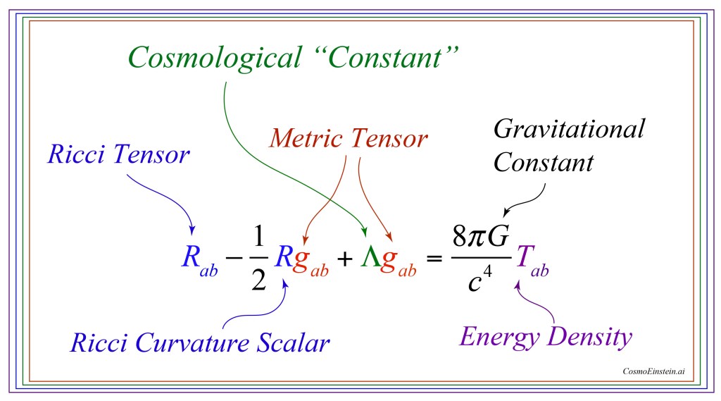
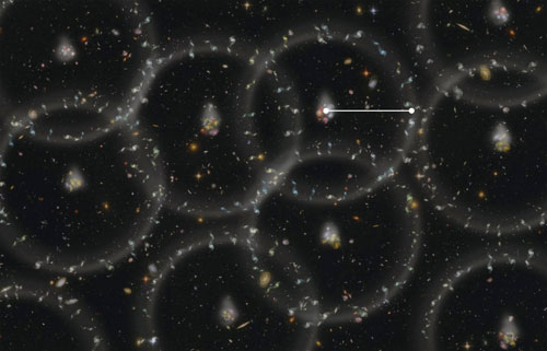
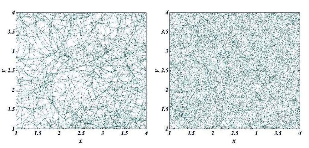
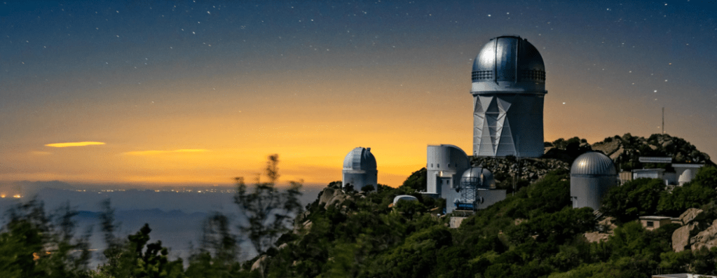
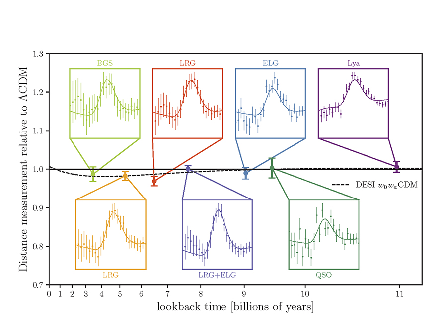
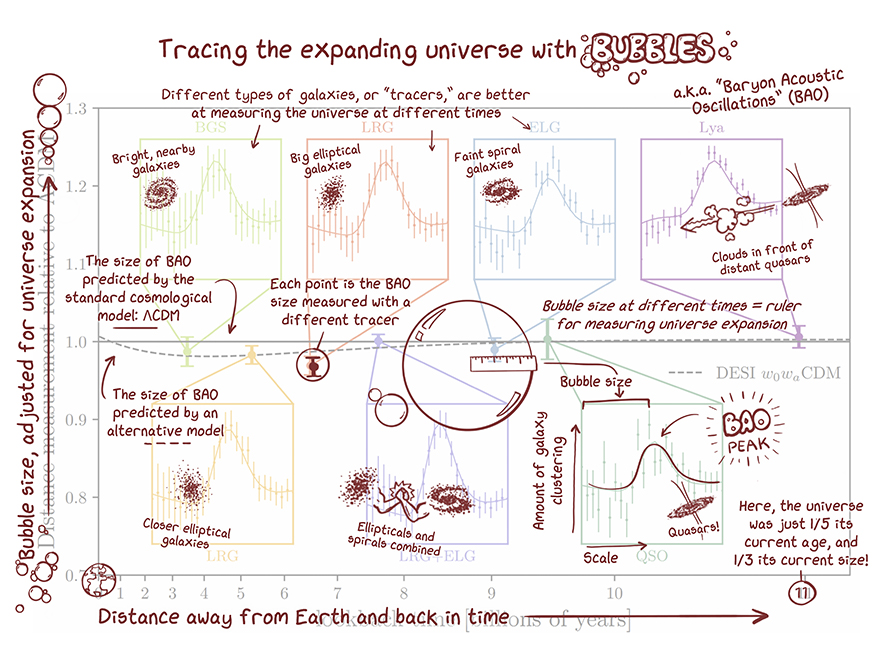


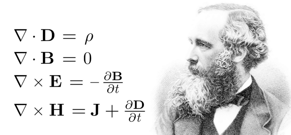
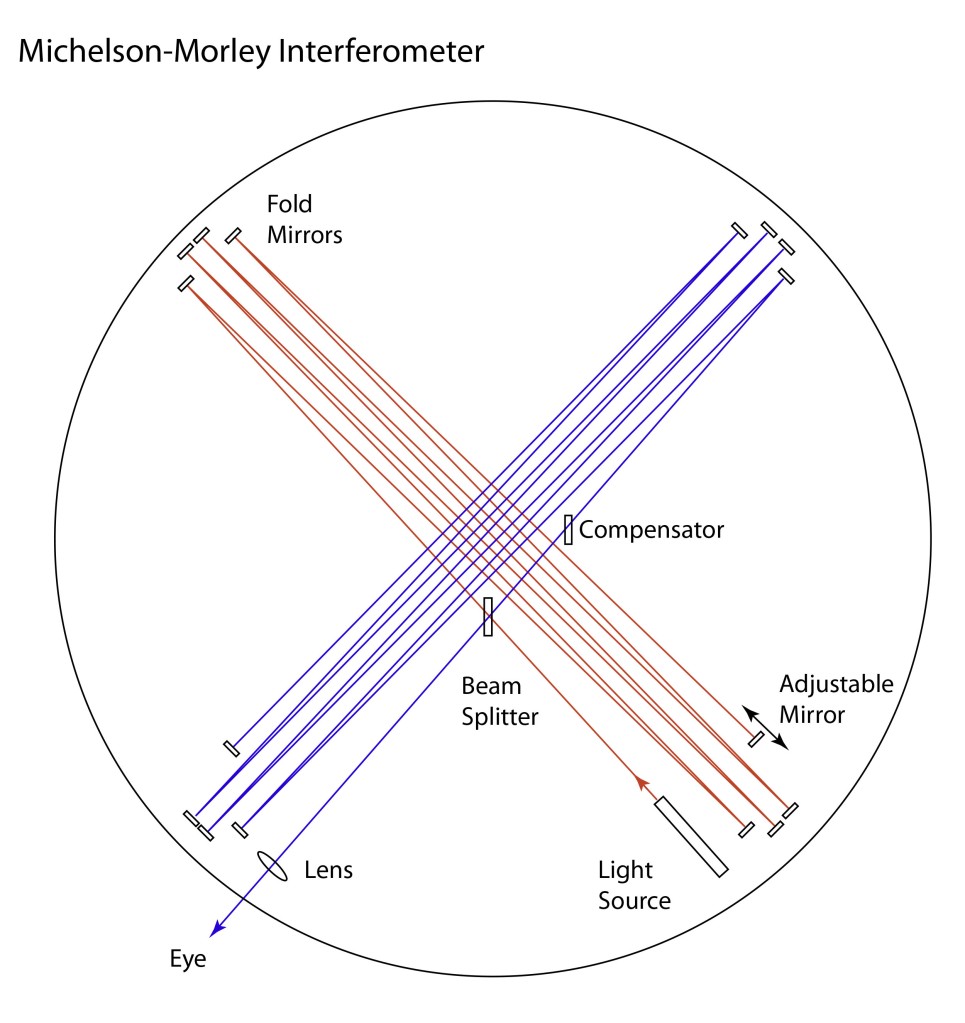
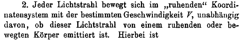
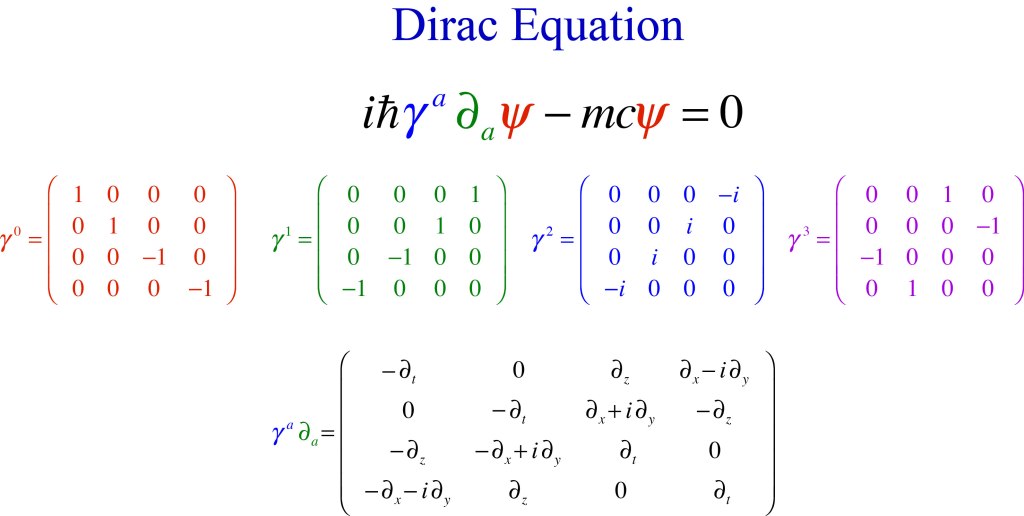
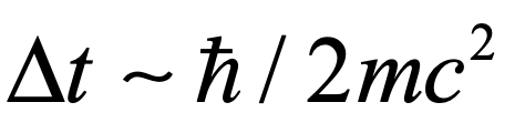
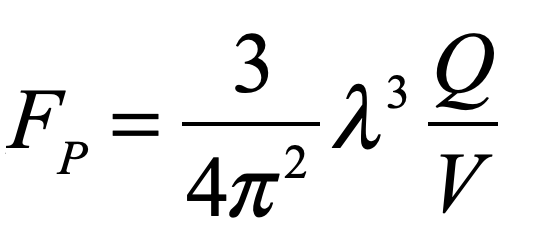
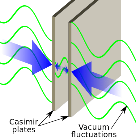


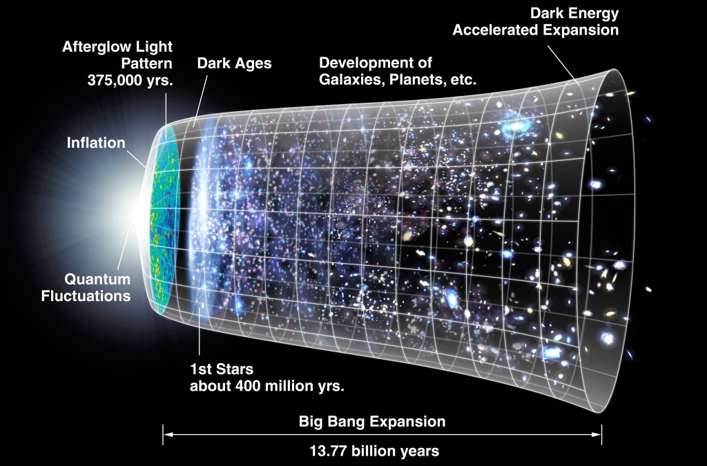


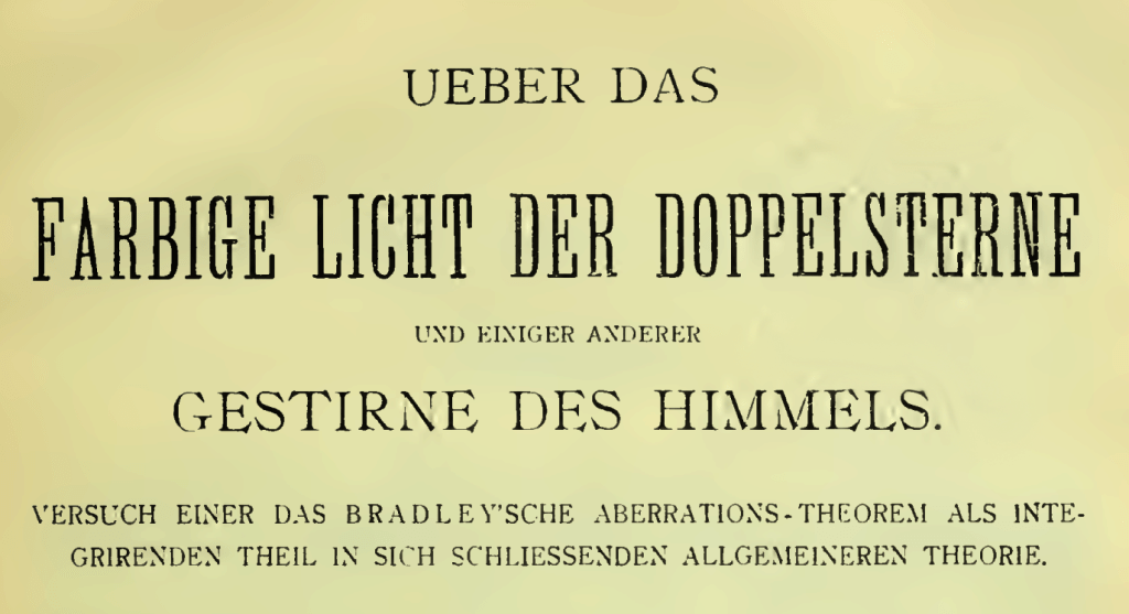
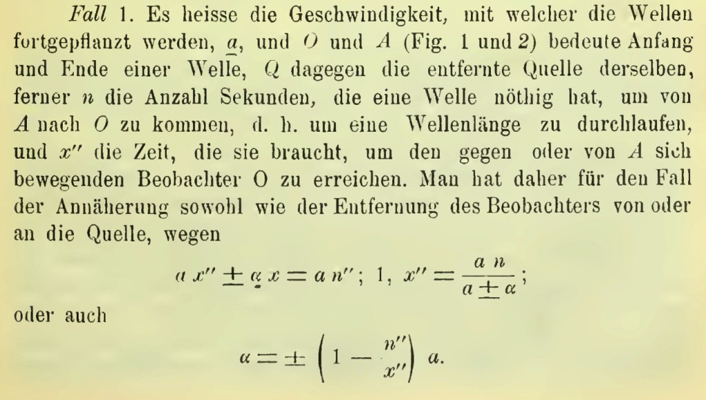

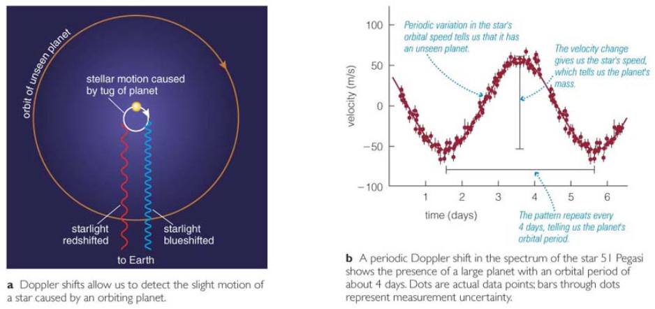
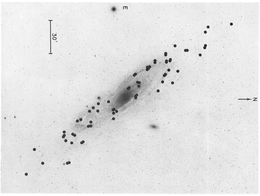
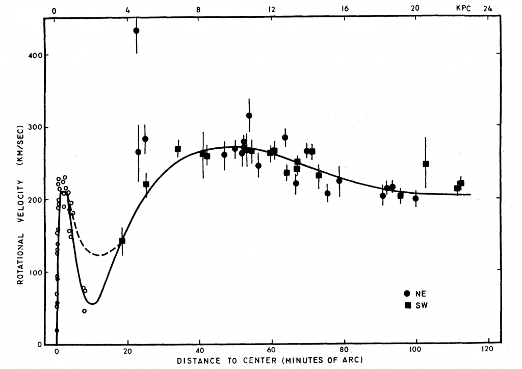

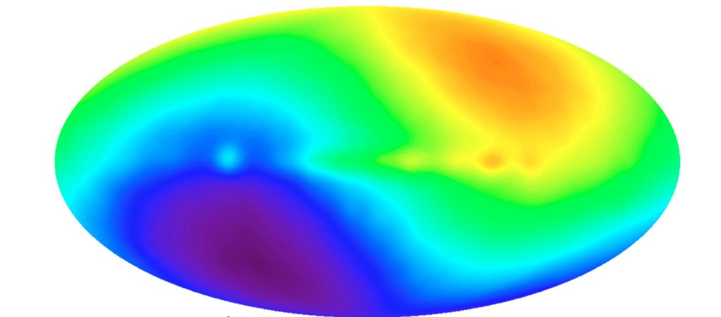
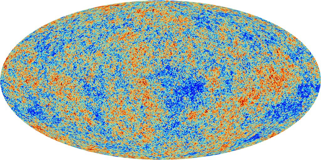
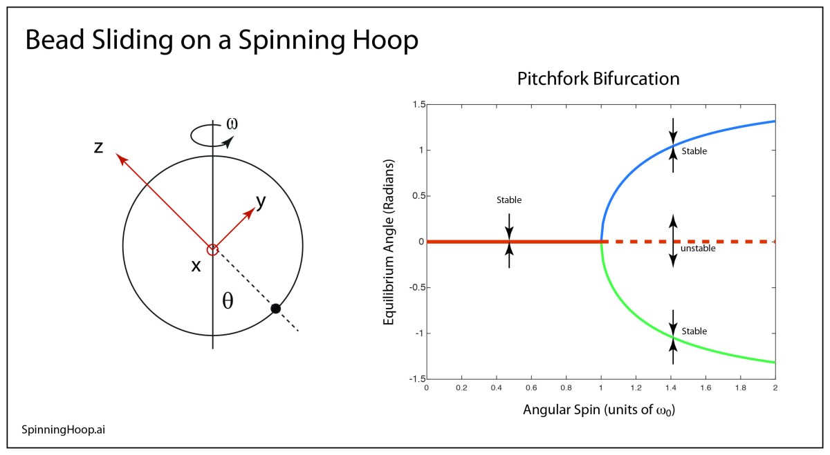

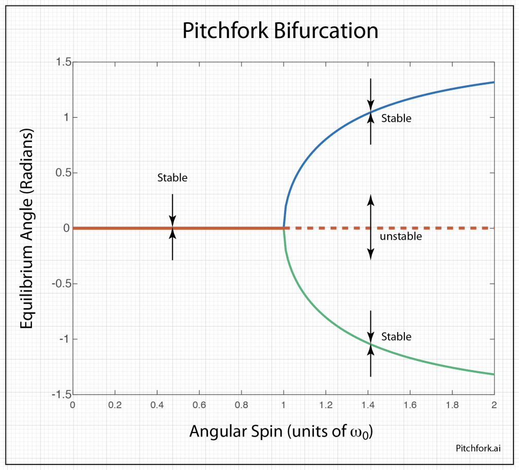
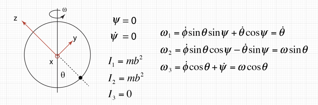
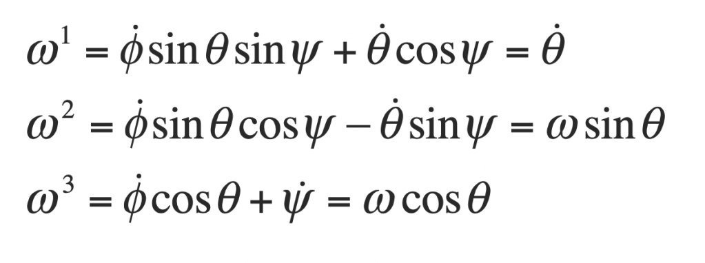
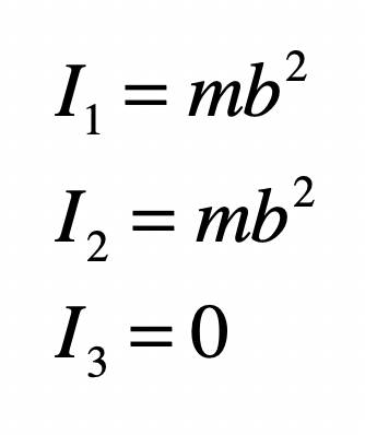
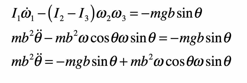
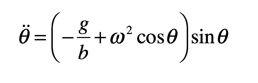
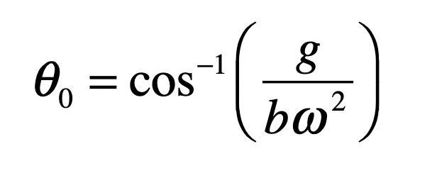
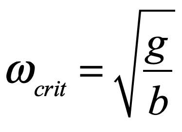
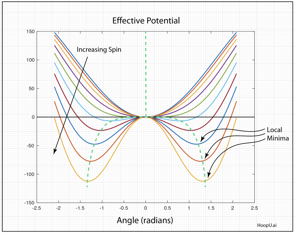
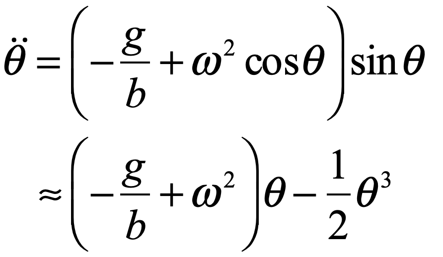
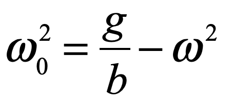
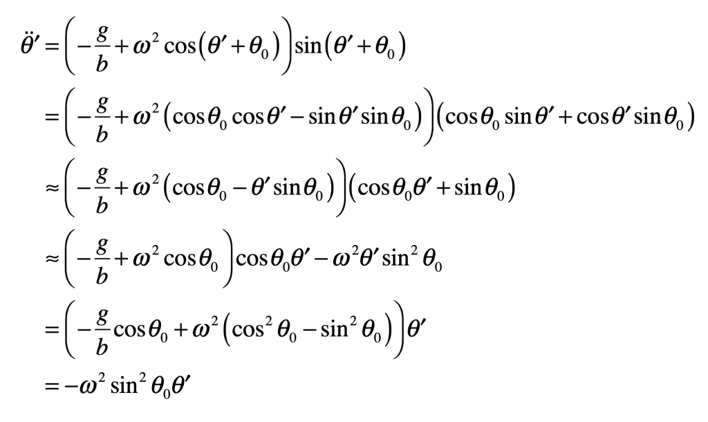
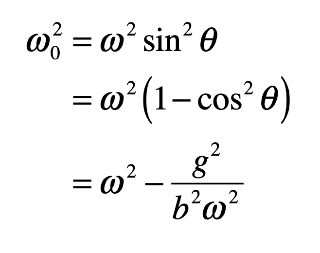
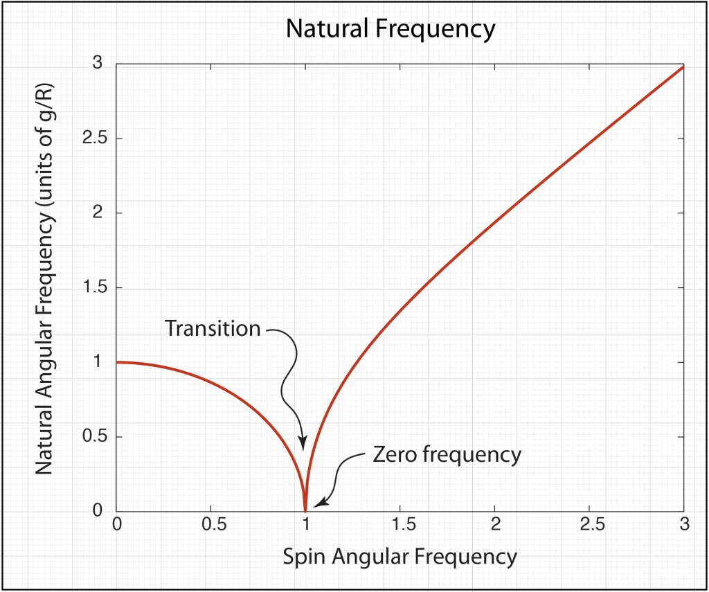
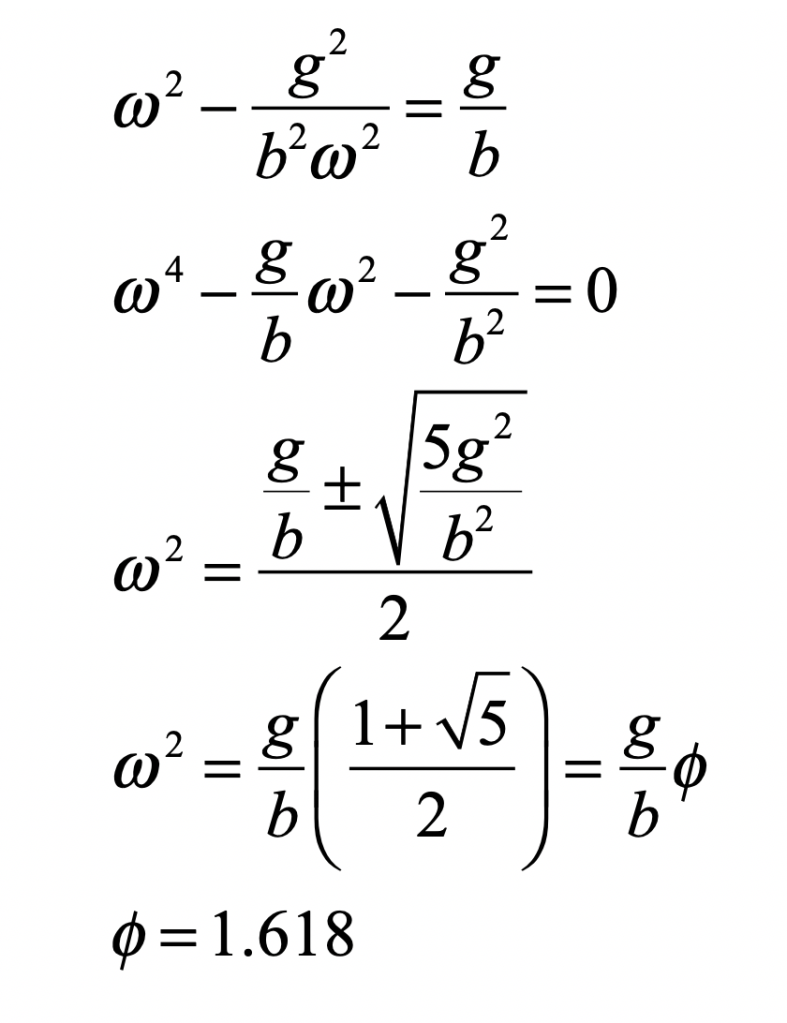


