It’s amazing what a little house arrest can do for the active mind. It provides time and focus as well as protection from earthly distractions that dissipate the intellect. How much more productive might we be if freed from the daily grind?
For Galileo Galilei, house arrest after ridiculing the pope gave him time to write his “Two New Sciences” that had been percolating in the back of his mind for decades. His arrest gave birth to the sciences of mechanics and strength of materials.
For Augustin Fresnel, house arrest after supporting royalists against Napoleon was the perfect retreat from building roads and bridges to explore the physics of light scattering and interference. His arrest gave birth to the physics of optical interference.
For Jean-Victor Poncelet, whiling away his time as a prisoner of war in Russia after Napoleon’s disastrous march on Moscow, it kept him occupied and sane. His confinement gave birth to the theory of projective geometry.
For Piotr Kapitsa, exiled under Stalin for not joining the Party, he could focus on his physics. His arrest gave birth to the physics of dynamic equilibrium.
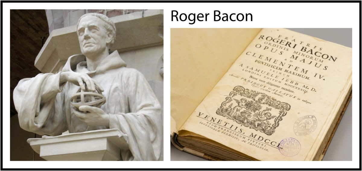
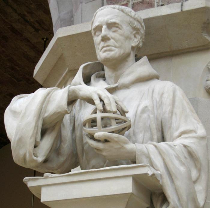
For Roger Bacon (121? – 1292), the medieval Franciscan friar who was under effective house arrest (his monastic cell) and prohibited from publishing anything, his arrest gave birth to the first science grant proposal.
The Rise of Roger Bacon
More has been written about Roger Bacon that is fantasy than the truth. In truth, almost nothing is known of his background, other than that he came from a wealthy family. They paid for him to go to college, at the age of thirteen, at Oxford, where he studied until he received his magister’s degree around 1240. Because Oxford was a religious college, his degree allowed him to teach anywhere under the umbrella of the Catholic Church, whether in Bologna, Rome, Paris or Oxford. Latin was the universal language, and the Christian faith was the universal context of all the young universities, so that scholars could move at will among these great centers of learning, despite the constant wars that raged between England and France. Bacon began teaching at Oxford, but the university in Paris at that time removed their prohibition against the teaching of Aristotle’s science, so he was recruited in 1241 to teach science in the Faculty of Arts, in the English division of the University of Paris.
During his time in Paris, across seven years, starting when he was around 30 years old, he began to shift his perspective on the state of learning in the university system. At that time, scholarly discourse was based on creative citation of the authorities, much like discourse is in law, citing court cases and legal precedence. New ideas arose by finding ambiguities or contradictions in established texts and then arguing for a new theory that could explain or contain formerly conflicting points of view. This kind of learning was endlessly self-referential and backwards focused, never moving forward beyond the frontiers of what was known.
At Paris, he met Peter Peregrinus, whose open-mindedness came as a revelation to Bacon. Peregrinus was willing to study anything, no mater how arcane (even magic tricks), burrowing down to the finest detail to understand how it worked. This meant using direct observation in place of cited authorities as the foundation for creating new ideas that could explain what was observed. At the time this was a radical departure, because it meant that the realm of knowledge could be added to, not just refined. It also elevated the individual to the level of the ancient authorities in their ability to devine new truths about nature. These new attitudes about observation and experimentation were reinforced when Bacon returned to Oxford in 1247 where he was exposed to the ideas of Robert Grosseteste.
Grosseteste and Bacon at Oxford
Robert Grosseteste (1170 – 1251) was born poor but his brilliance must have been recognized early by some priest with influence, because his education was supported by the Church. He was educated at Oxford and began teaching there, rising through the ranks to become the Magister Scholarum (Master of the Schools … like Chancellor) of Oxford University in 1215, a position he held for six years. This high office allowed him a latitude of thought that would have been impossible in a lesser position, and he slowly changed the mindset at the university away from the verbal arguments of Scholasticism.
Teaching at Oxford focused on the quadrivium (geometry, arithmetic, music, and astronomy), which was not “science” as we would understand it today, but it had some of the ingredients. Grosseteste emphasized the importance of observation of nature to test theoretical predictions, and he enlisted geometry and arithmetic as tools to describe observations. These both were innovations over the previous Scholastic emphasis of pure reason divorced from direct experience (eperimentum). Grosseteste’s favorite topic for observation and experience was the natural behavior of light and optics, in part because the behavior of rays of light could be captured using geometry.
Grosseteste stepped down from the chancellory in 1221 to teach at Franciscan monasteries that were closely associated with university life. He was still teaching there at the time when Bacon entered Oxford, but it is not known if they ever had an association. By the time Bacon returned to Oxford in 1247, Grosseteste had moved on to become the Bishop of Lincoln, but his legacy of natural philosophy was firmly embedded in the mindset of the faculty teaching the quadrivium.
After arriving back at Oxford, Bacon embraced Grosseteste’s teachings and began systematically expanding on them. From Grosseteste, he adopted the need to validate theory by direct experience, to use of mathematics to describe phenomena, and he chose the study of light and optics as the prime example of the new approach. He used his access to his family’s wealth to buy an extremely large assortment of books and tables and instruments. The value of these purchases today would be in the range of a million dollars or so; it was a vast collection of academic value. He was an independent scholar, and independently wealthy, so it is hard to understand why, a few years later in 1251, he joined the Franciscan Order with its vow of severe poverty.
It may have been Grosseteste’s association with the Franciscans (although Grosseteste never joined the order himself), or the close association of the Franciscans with higher learning. It may also have been because Bacon was accumulating enemies as he pushed Grosseteste’s ideas to more radical extremes. Bacon was known to be arrogant and caustic, and his willingness to entertain new ideas, possibly going against traditional Church doctrine, was putting him more at risk at a time when deviating from doctrine could be physically dangerous. Joining the Franciscans might have been a sort of protection for him, though he would have had to give up his collection of books, tables and instruments because of the poverty vow. At first, this seemed a shrewd move, but in time it unravelled into a personal nightmare.
Roger Bacon in Crisis
The Church has always been buffeted by the persistent emergence of heresies against doctrine, and it always has worked to stamp them out. Around the time of Bacon, the most dangerous heresy was Joachimism, or the heresy of the Eternal Gospel. It had strange ideas about the Apocolypse that did not sit well with Church teachings, so it was aggressively banned. Unfortunately, many Franciscan academics were in the thick of it, and they were also in a position to publish books about it. In 1256, only 5 years after joining the Franciscan order, the new leader of the order banned writing on any unsanctioned topic, trapping Bacon with no publishable outlet for his ideas. But that didn’t stop him from talking.
In 1264, the French lawyer and diplomat Cardinal Guy de Foulques was in England to mediate between Henry III and his barons who were on the edge of revolt over Henry’s abuse of power. During a quiet period in the negotiations, Bacon and de Foulques met and talked. It was a rare outlet for Bacon who had been pent up for years. He impressed de Foulques with his wide-ranging ideas about education reform to move beyond the stagnation of Scholasticism. Bacon argued for an emphasis on science and math as a way to uncover natures secrets, and he promoted the learning of languages (Arabic and Hebrew and Greek) to better learn from all the intellectual output of other cultures. It must have been a heady conversation, and Bacon was probably thrilled to have such an esteemed listener. But his own life was poised on disaster.
Three events collapsed Bacon’s world around him. First, despite de Fulques efforts, negotiations broke down and the Second Baron’s War broke out. Second, Bacon’s wealthy family supported the king but were overrun by the Barons and ruined. Third, Bacon and his ideas were now deemed too dangerous by his Franciscan superiors, and he was sent to a convent outside of Paris in effective house arrest as his days were filled with menial tasks purposely meant to exhaust him and give him no time to think.
One year into the war and into Bacon’s exile to Paris, Cardinal de Fulques was elected pope as Clement IV. He took up the mantel of Christ just as Christianity was in retreat on multiple fronts. In the northeast it was under assault by the terrifying and highly successful Mongol invasion, in the southwest by a military incursion into Spain from Moorish Morroco, and in the Levant by the Mamluk Sultanate as they recaptured the last Christian outposts from the Crusades. Clement needed help, and he never forgot his conversation with Bacon about how to use science and math to give the Christian forces the upper hand. At the time of their talk, Bacon had been so persuasive while pitching his ideas so hard, that Clement had walked away with the impression that it was all already written up. So he sent a letter to Bacon in Paris asking for an immediate report on the status of Bacon’s program. That letter was a trigger for one of the most astounding bursts of creative scholarship of the Middle Ages. It was also the trigger for what may be called the first scientific grant proposal.
Roger Bacon’s Opus
When the Pope’s letter arrived in Paris, Bacon was ten years into the Franciscan prohibition against publishing and two years into his sentence of menial labor. To respond to the Pope’s request was both a dream and nightmare. It was a dream, because it gave Bacon the ear of the most powerful person in Europe and an outlet for all his pent up ideas. It was a nightmare, because he had no time to do the work and no resources to accomplish it.
To create a manuscript in the 13th century was a long and expensive process that required funds to buy materials. His family had just been ruined financially in the Baron’s war, so he secretly turned to friends to help support the project. He also worked mostly at night while spending his days on all his duties at the convent.
His central thesis was clear: Christian forces were in retreat because their enemies had both technological and logistical superiority. To gain the upper hand in the fight required a reform of teaching across Europe. By better understanding the laws of nature through math and science, they could develop technologically superior weapons. By better understanding languages, they would have access to learning from other cultures. By better understanding moral philosophy, they would gain the advantage of the moral high ground.
To show how to put these ideas into practice, Bacon chose specific examples. He picked the study of optics (perspectiva) as a way to practice detailed observation and mathematical description of physical phenomena. He promoted the questioning of authority as a way to escape the ruts of old thinking, opening the mind to new possibilities. He championed astronomy and calendar reform to stop the seasons from drifting across the years and to improve logistic planning. He supported geography as a way to better understand where future threats might emerge.
In a little over one year, Bacon wrote four manuscripts that contained nearly a million words in total. To put that in perspective, a typical academic book published today has about 100,000 words. Therefore, Bacon wrote in one year the equivalent of about 10 academic books at a time without word processors and without paper, all written by hand in permanent ink on expensive parchment. This output was put into three works — the Opus Majus, the Opus Minus and the Opus Tertium — plus a fourth manuscript that was the first of its kind: the grant proposal.
The Letter on the Secret Works of Art and Nature
The primary purpose of Bacon’s response to the Pope was to ask him to fund research. The Opus, despite its massive size, was simply an outline that needed to be filled in, an activity that required time and money and freedom (as a way to escape his house arrest). Bacon was approaching the age of 50 and his time was running out. Life expectancy for someone who survived childhood in the 13th century was only about 55 years.
To clearly communicate the urgency of his program and the advantages that could be gained by adopting it, Bacon wrote Epistola de Secretis Operibus (Letter on the Secret Works of Art and Nature). He took out all the stops and let his imagination run free to describe what might be possible with applied physics.
Bacon envisioned machines that would move mechanically across land or water without the need for human power (automobiles and ships). He suggested other machines that could move secretly under water to surprise an enemy (submarines). He even imagined machines that could transport a man through the air, speeding him across a battlefield (airplanes). From the study of optics, he proposed the ability to make far things appear close (telescopes). From the study of mechanics, he envisioned bridges that could span great distances (suspension bridge), and systems that could support weights much larger than could be lifted by man (mechanical and civil engineering). And he gave the formula for a chemical mixture that could destroy the walls of cities (gunpowder).
The letter reads like the classic section of a grant proposal that lists potential benefits. He may have been looking far into the future, much farther than we do now when we write modern grant proposals, but his reasoning was surprisingly sound, based on the knowledge that would be gained by studying the laws of nature, i.e., science.
Unfortunately, shortly after Bacon secretly delivered his works to the Pope through a trusted student, the Pope died, possibly never having read any of it. Worse, Bacon was later imprisoned in Italy, placed in solitary confinement for ten years because of fear of his radical ideas. He was finally released, around the age of 80, never having accomplished his grand program. He died two years later at his beloved Oxford.