
“By rights, we shouldn’t even be here,” says Samwise Gamgee to Frodo Baggins in the Peter Jackson movie The Lord of the Rings: The Two Towers.
But we are!
We, our world, our Galaxy, our Universe of matter, should not exist. The laws of physics, as we currently know them, say that all the matter created at the instant of the Big Bang should have annihilated with all the anti-matter there too. The great flash of creation should have been followed by a great flash of destruction, and all that should be left now is a faint glow of light without matter.
Except that we are here, and so is our world, and our Galaxy and our Universe … against the laws of physics as we know them.
So, there must be more that we have yet to know. We are not done yet with the laws of physics.
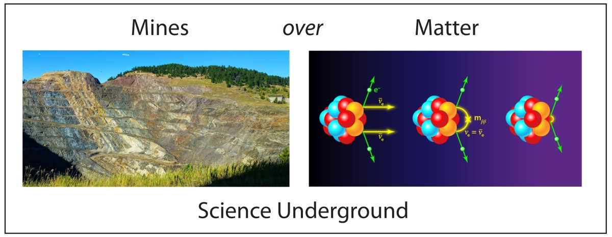
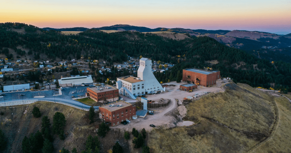
Which is why the scientists of the Sanford Underground Research Facility (SURF), a kilometer deep under the Black Hills of South Dakota, are probing the deep questions of the universe near the bottom of a century-old gold mine.
Homestake Mine
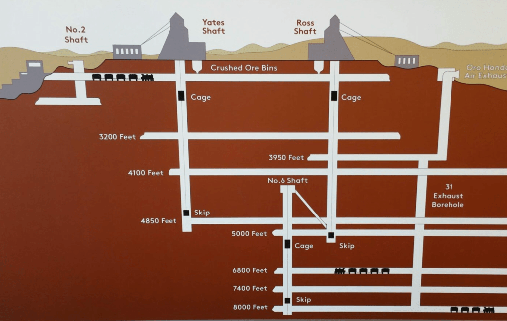
>>> Twenty of us are plunging vertically at one meter per second into the depths of the earth, packed into a steel cage, seven to a row, dressed in hard hats and fluorescent safety vests and personal protective gear plus a gas filter that will keep us alive for a mere 60 minutes if something goes very wrong. It is dark, except for periodic fast glimpses of LED-lit mine drifts flying skyward, then rock again, repeating over and over for ten minutes. Drops of water laced with carbonate drip from the cage ceiling, that, when dried, leave little white stalagmites on our clothing. A loud bang tells everyone inside that a falling boulder has crashed into the top of the cage, and we all instinctively press our hard hats more tightly onto our heads. Finally, the cage slows, eventually to a crawl, as it settles to the 4100 level of the Homestake mine. <<<
The Homestake mine was founded in 1877 on land that had been deeded for all time to the Lakota Sioux by the United States Government in the Treaty of Fort Laramie in 1868—that is, before George Custer, twice cursed, found gold in the rolling forests of Ȟe Sápa—the Black Hills, South Dakota. The prospectors rushed in, and the Lakota were pushed out.
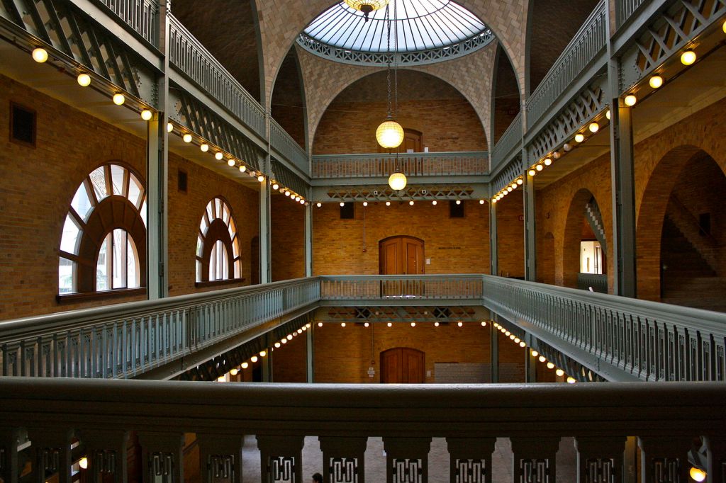
Gold was found washed down in the streams around the town of Deadwood, but the source of the gold was found a year later at the high Homestake site by prospectors. The stake was too large for them to operate themselves, so they sold it to a California consortium headed by George Hearst, who moved into town and bought or stole all the land around it. By 1890, the mine was producing the bulk of gold and silver in the US. When George Hearst died in 1891, his wife Phoebe donated part of the fortune to building projects at the University of California at Berkeley, including the Hearst Mining Building, which was the largest building devoted to the science of mining engineering in the world. Their son, William Randolph Hearst, became a famous newspaper magnate and a possible inspiration for Orson Well’s Citizen Cane.
By the late 1900’s, the mining company had excavated over 300 miles of tunnels and extracted nearly 40 million ounces of gold (equivalent to $100B today). Over the years, the mine had gone deeper and deeper, eventually reaching the 8000 foot level (about 3000 feet below sea level).
This unique structure presented a unique opportunity for a nuclear chemist, Ray Davis, at Brookhaven National Laboratory who was interested in the physics of neutrinos, the elementary particles that Enrico Fermi had named the “little neutral ones” that accompany radioactive decay.
Neutrinos are unlike any other fundamental particles, passing through miles of solid rock as if it were transparent, except for exceedingly rare instances when a neutrino might collide with a nucleus. However, neutrino detectors on the surface of the Earth were overwhelmed by signals from cosmic rays. What was needed was a thick shield to protect the neutrino detector, and what better shield than thousands of feet of rock?
Davis approached the Homestake mining company to request space in one of their tunnels for his detector. While a mining company would not usually be receptive to requests like this, one of its senior advisors had previously had an academic career at Harvard, and he tipped the scales in favor of Davis. The experiment would proceed.
The Solar Neutrino Problem
>>> After we disembark onto the 4100 level (4100 feet below the surface) from the Ross Shaft, we load onto the rail cars of a toy train, the track width little more than a foot wide. The diminutive engine clunks and clangs and jerks itself forward, gathering speed as it pushes and pulls us, disappearing into a dark hole (called a drift) on a mile-long trek to our experimental site. Twice we get stuck, the engine wheels spinning without purchase, and it is not clear if the engineers can get it going again.
At this point we have been on the track for a quarter of an hour and the prospect of walking back to the Ross is daunting. The only other way out, the Yates Shaft, is down for repairs. The drift is unlit except by us with our battery-powered headlamps sweeping across the rock face, and who knows how long the batteries will last? The ground is broken and uneven, punctuated with small pools of black water. There would be a lot of stumbling and falls if we had to walk our way out. I guess this is why I had to initial and sign in twenty different places on six pages, filled with legal jargon nearly as dense as the rock around us, before they let me come down here. <<<
In 1965, the Homestake mining crews carved out a side cavern for Davis near the Yates shaft at the 4850 level of the mine. He constructed a large vat to hold cleaning fluid that contained lots of chlorine atoms. When a rare neutrino interacted with a chlorine nucleus, the nucleus would convert to argon and give off a characteristic flash of light. By tallying the flashes of light, and by calculating how likely it was for a neutrino to interact with a nucleus, the total flux of neutrinos through the vat could be back calculated.
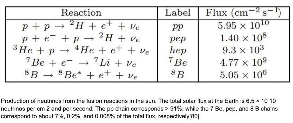
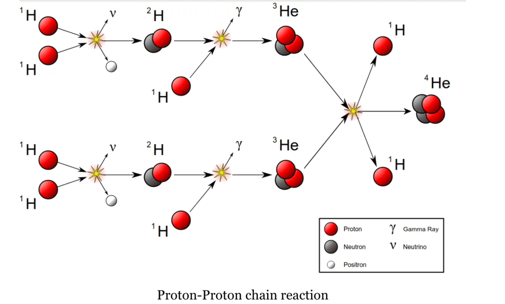
The main source for neutrinos in our neck of the solar system is the sun. As hydrogen fuses into helium, it gives off neutrinos. These pass through the overlying layers of the sun and pass through the Earth and through Davis’ vat—except those rare cases when chlorine converts to argon. The rate at which solar neutrinos should be detected in the vat was calculated very accurately by John Bahcall at Cal Tech.
By the early 1970’s, there were enough data that the total neutrino flux could be calculated and compared to the theoretical value based on the fusion reactions in the sun—and they didn’t match. Worse, they didn’t match within a factor of three! There were three times fewer neutrino events detected that there should have been. Where were all the missing neutrinos?
This came to be called the “Solar neutrino problem”. At first, everyone assumed that the experiment was wrong, but Davis knew he was right. Then others said the theoretical values were wrong, but Bahcall knew he was right. The problem was, that Davis and Bahcall couldn’t both be right, could they?
Enter neutrino oscillations.
The neutrinos coming from the sun originate mostly as what are known as electron neutrinos. These interact with a neutron in a chlorine nucleus to convert it to a proton plus an ejected electron. But if the neutrino were of a different kind, perhaps a muon neutrino, then there isn’t enough energy for the neutron to eject a muon, so the reaction doesn’t take place.
This became the leading explanation for the missing solar neutrinos. If many of them converted to muon neutrinos on their way to the Earth, then the Davis experiment wouldn’t detect them—hence the missing events.
The way that neutrinos can oscillate from electron neutrinos to muon neutrinos is if neutrinos have a very small but finite mass. This was the solution, then, to the solar neutrino problem. Neutrinos have mass. Ray Davis was awarded the Nobel Prize in Physics in 2002 for his discovery of the missing neutrinos.
But one solution begets another problem: the Standard Model of elementary particles says that neutrinos are massless. What can be going on with the Standard Model?
Once again, the answer may be found deep underground.
Sanford Underground Research Facility (SURF)
>>> The rock of the Homestake is one of the hardest and densest rocks you will find, black as night yet shot through with white streaks of calcite like the tails of comets. It is impermeable, and despite being so deep, the rock is surprisingly dry—most of the fractures are too tight to allow a trickle through.
As our toy train picks up speed, the veins flash by in our headlamps, sometimes sparkling with pin pricks of reflected light. A gold fleck perhaps? Yet the drift as a whole (or as a hole) is a shabby thing, rusty wedges half buried in the ceiling to keep slabs from falling, bent and battered galvanized metal pinned to the walls by rock bolts to hold them back, flimsy metal webbing strung across the ceiling to keep boulders from crushing our heads. It’s dirty and dark and damp and hewn haphazardly from the compressed crust. There is no art, no sense of place. These shafts were dynamited through, at three-to-five feet per detonation, driven by money and the need for the gold, so nobody had any sense of aesthetics. <<<
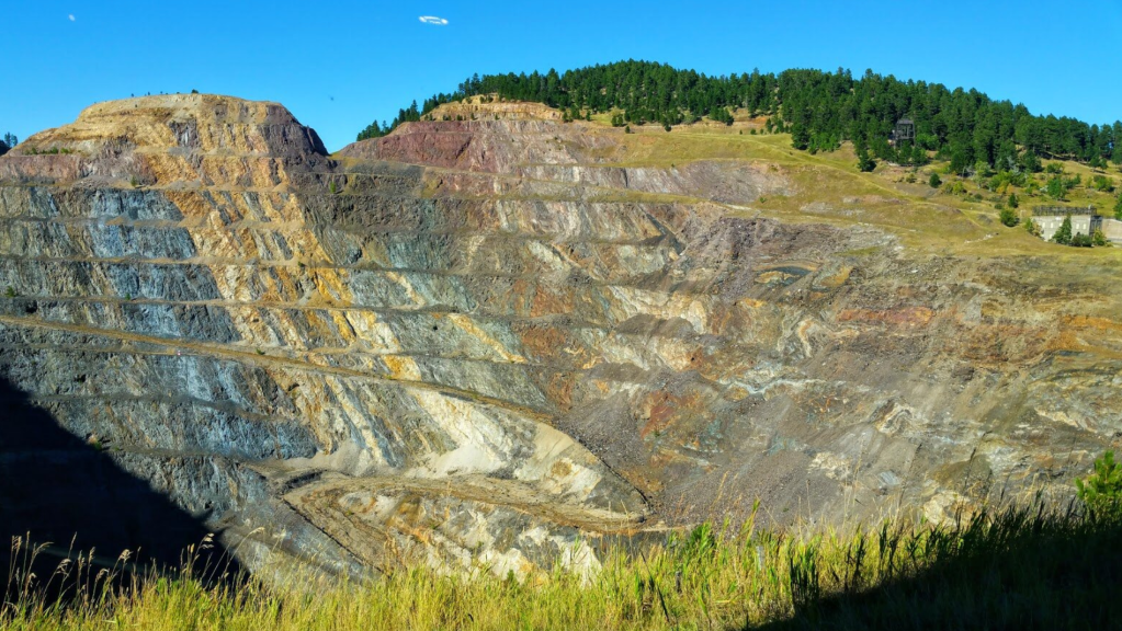
The Homestake mine closed operations in 2001 due to the low grade of ore and the sagging price of gold. They continued pumping water from the mine for two more years in anticipation of handing the extensive underground facility over to the National Science Foundation for use as a deep underground science lab. However, delays in the transfer and the cost of pumping forced them to turn off the pumps and the water slowly began rising through the levels, taking a year or more to rise and flood the famous 4850 level while negotiations continued.
Finally, the NSF took over the facility to house the Deep Underground Science and Engineering Laboratory (DUSEL) that would operate at the deepest levels, but these had already been flooded. After a large donation from South Dakota banker T. Denny Sanford and support from the Governor Mike Rounds, the facility became the Sanford Underground Research Fability (SURF). The 4850 level was “dewatered”, and the lab was dedicated in 2009. But things were still not settled. NSF had second thoughts, and in 2011 the plans for DUSEL (still under water) were terminated and the lab was transferred to the Department of Energy (DOE), administered through the Lawrence Berkeley National Laboratory, to host experiments at the 4850 level and higher.
Two early experiments at SURF were the Majorana Demonstrator and LUX.
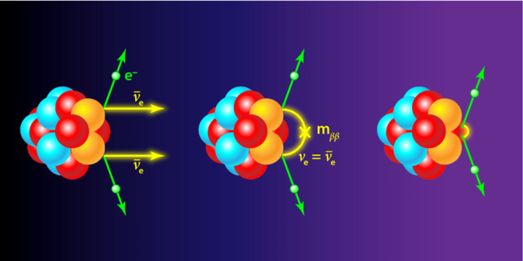
The Majorana Demonstrator was an experiment designed to look for neutrino-less double-beta decay where two neutrons in a nucleus decay simultaneously, each emitting a neutrino. A theory of neutrinos proposed by the Italian physicist, Ettore Marjorana, in 1937 that goes beyond the Standard Model ,says that a neutrino is its own antiparticle. If this were the case, then the two neutrinos emitted in the double beta decay could annihilate each other—hence a “neutrinoless” double beta decay. The Demonstrator was too small to actually see such an event, but it tested the concept and laid the ground for later larger experiments. It operated between 2016 and 2021.
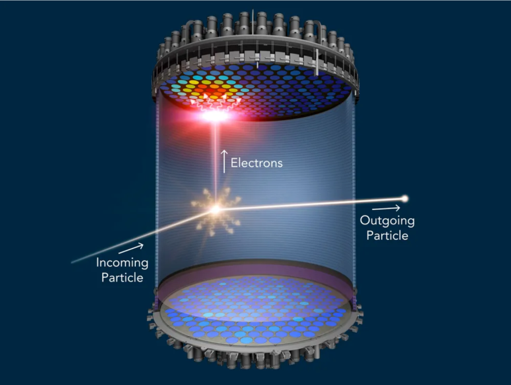
The Large Underground Xenon (LUX) experiment was a prototype for the search for dark matter. Dark matter particles are expected to interact very weakly with ordinary matter (sort of like neutrinos, but even less interactive). Such weakly interacting massive particles (WIMPs) might scatter off a nucleus in an atom of Xenon, shifting the nucleus enough that it emits electrons and light. These would be captured by detectors at the caps of the liquid Xenon container.
Once again, cosmic rays at the surface of the Earth would make the experiment unworkable, but deep underground there is much less background within which to look for the “needle in the haystack”. LUX operated from 2009 to 2016 and was not big enough to hope to see a WIMP, but like the Demonstrator, it was a proof-of-principle to show that the idea worked and could be expanded to a much larger 7-ton experiment called LUX-Zeplin that began in 2020 and is ongoing, looking for the biggest portion of mass in our universe. (About a quarter of the energy of the universe is composed of dark matter. The usual stuff we see around us only makes up about 4% of the energy of the universe.)
Deep Underground Neutrino Experiment (DUNE)
>>> “Always keep a sense of where you are,” Bill the geologist tells us, in case we must hike our way out. But what sense is there? I have a natural built-in compass that has served me well over the years, but it seems to run on the heavens. When I visited South Africa, I had an eerie sense of disorientation the whole time I was there. When you are a kilometer underground, the heavens are about as far away as Heaven. There is no sense of orientation, only the sense of lefts and rights.
We were told there would be signs directing us towards the Ross or Yates Shafts. But once we are down here, it turns out that these “signs” are crudely spray-painted marks on the black rock, like bad graffiti. When you see them, your first thought is of kids with spray cans making a mess—until you suddenly recognize an R or an O or two S’s along with an indistinct arrow that points slightly more one way than the other. <<<

One of the most ambitious high-energy experiments ever devised is the Long Baseline Neutrino Facility (LBNF) that is 800 miles long. It begins in Batavia, Illinois, at the Fermilab accelerator that launches a beam of neutrinos that travel 800 miles through the Earth to detectors at the Deep Underground Neutrino Experiment (DUNE) at SURF in Lead, South Dakota. The neutrinos are expected to oscillate in flavor, just like solar neutrinos, and the detection rates at DUNE could finally answer one of the biggest outstanding questions of physics: Why is our universe made of matter?
At the instant of the Big Bang, equal amounts of matter and antimatter should have been generated, and these should have annihilated in equal manner, and the universe should be filled with nothing but photons. But it’s not. Matter is everywhere. Why?
In the Standard Model there are many symmetries, also known as conserved properties. One power symmetry is known as CPT symmetry, where C is a symmetry of changing particles into the antiparticles, P is a reflection of left-handed or right-handed particles, and T is time-reversal symmetry. Yet there could be a CP symmetry too, which you might expect if time-reversal is taken as a symmetric property of physics. But it’s not!
There is a strange meson called a Kaon that does not decay the same way for its particle and antiparticle pair, violating CP symmetry. This was discovered in 1964 by James Cronin and Val Fitch who won the 1980 Nobel prize in physics. The discovery shocked the physics world. Since then, additional violations of CP symmetry have been observed in quarks. Such a broken symmetry is allowed in the Standard Model of particles, but the effect is so exceedingly small—CP is so extremely close to being a true symmetry—that it cannot explain the size of the matter-antimatter asymmetry in the universe.
Neutrino oscillations also can violate CP symmetry, but the effects have been hard to measure—thus the need for DUNE. By creating large amounts of neutrinos, beaming them 800 miles through the Earth, and detecting them in the vast liquid Argon vats in the underground caverns of SURF, the parameters of neutrino oscillation can be measured directly, possibly explaining the matter asymmetry of the universe—and answering Samwise’s question of why we are here.
Center for Understanding Subsurface Signals and Permeability (CUSSP)
>>> Finally, in the distance, as we rush down the dark drift, we see a bright glow that grows to envelope us with a string of white LED lights. The drift is not so shabby here, with fresh pipes and electrical cables laid neatly by the side. We had arrived at the CUSSP experimental site. It turned out it was just a few steps away from the inactive Yates Shaft, that, if it had been operating, would have removed the need for the crazy train ride through black rock along broken tunnels. But that is OK. Because we are here, and this is what had brought us down into the Earth to answer questions down-to-Earth as we try to answer questions related to our future existence on this planet, learning what we need to generate the power for our high-tech society without making our planet unlivable. <<<
Not all the science at SURF is so ethereal. For instance, research on Enhanced Geothermal Systems (EGS) is funded by the DOE Office of Basic Energy Sciences. Geothermal systems can generate power by extracting super-heated water from underground to run turbines. However, superheated water is nasty stuff, very corrosive and full of minerals that tend to block up the fractures that the water flows through. The idea of enhanced geothermal systems is to drill boreholes and use “fracking” to create fractures in the hard rock, possibly refracturing older fractures that had become blocked. If this could be done reliably, then geothermal sites could be kept operating.
The Center for Understanding Subsurface Signals and Permeability (CUSSP) was recently funded by the DoE to use the facilities at SURF to study how well fracks can be controlled. The team is led by Pacific Northwest National Lab (PNNL) with collaborations from Lawrence Berkeley Lab, Maryland, Illinois and Purdue, among others. We are installing seismic equipment as well as electrical resistivity to monitor the induced fractures.
The CUSSP installation on the 4100 level was the destination of our underground journey, to see the boreholes in person and to get a sense of the fracture orientations at the drift wall. During the half hour at the site, rocks were examined, questions were answered, tall tales were told, and it was time to return.
Shooting to the Stars
>>> At the end of the tour, we pack again into the Ross cage and are thrust skyward at 2 meters per second—twice the speed as coming down because of the asymmetry of slack cables that could snag and snap. Ears pop, and pop again, until the cage slows, and we settle to the exit level, relieved and tired and ready to see the sky. Thinking back, as we were shooting up the shaft, I imagined that the cage would never stop, flying up past the massive hoist, up and onward into the sky and to the stars. <<<
In a video we had been shown about SURF, Jace DeCory, a scholar of the Lakota Sioux, spoke of the sacred ground of Ȟe Sápa—the Black Hills. Are we taking again what is not ours? This time it seems not. The scientists of SURF are linking us to the stars, bringing knowledge instead of taking gold. Jace quoted Carl Sagan: “We are made of star-stuff.” Then she reminded us, the Lakota Sioux have known that all along.


