These days, the physics breakthroughs in the news that really catch the eye tend to be Astro-centric. Partly, this is due to the new data coming from the James Webb Space Telescope, which is the flashiest and newest toy of the year in physics. But also, this is part of a broader trend in physics that we see in the interest statements of physics students applying to graduate school. With the Higgs business winding down for high energy physics, and solid state physics becoming more engineering, the frontiers of physics have pushed to the skies, where there seem to be endless surprises.
To be sure, quantum information physics (a hot topic) and AMO (atomic and molecular optics) are performing herculean feats in the laboratories. But even there, Bose-Einstein condensates are simulating the early universe, and quantum computers are simulating worm holes—tipping their hat to astrophysics!
So here are my picks for the top physics breakthroughs of 2023.
The Early Universe
The James Webb Space Telescope (JWST) has come through big on all of its promises! They said it would revolutionize the astrophysics of the early universe, and they were right. As of 2023, all astrophysics textbooks describing the early universe and the formation of galaxies are now obsolete, thanks to JWST.
Foremost among the discoveries is how fast the universe took up its current form. Galaxies condensed much earlier than expected, as did supermassive black holes. Everything that we thought took billions of years seem to have happened in only about one-tenth of that time (incredibly fast on cosmic time scales). The new JWST observations blow away the status quo on the early universe, and now the astrophysicists have to go back to the chalk board.
If LIGO and the first detection of gravitational waves was the huge breakthrough of 2015, detecting something so faint that it took a century to build an apparatus sensitive enough to detect them, then the newest observations of gravitational waves using galactic ripples presents a whole new level of gravitational wave physics.
By using the exquisitely precise timing of distant pulsars, astrophysicists have been able to detect a din of gravitational waves washing back and forth across the universe. These waves came from supermassive black hole mergers in the early universe. As the waves stretch and compress the space between us and distant pulsars, the arrival times of pulsar pulses detected at the Earth vary a tiny but measurable amount, haralding the passing of a gravitational wave.
This approach is a form of statistical optics in contrast to the original direct detection that was a form of interferometry. These are complimentary techniques in optics research, just as they will be complimentary forms of gravitational wave astronomy. Statistical optics (and fluctuation analysis) provides spectral density functions which can yield ensemble averages in the large N limit. This can answer questions about large ensembles that single interferometric detection cannot contribute to. Conversely, interferometric detection provides the details of individual events in ways that statistical optics cannot do. The two complimentary techniques, moving forward, will provide a much clearer picture of gravitational wave physics and the conditions in the universe that generate them.
Phosphorous on Enceladus
Planetary science is the close cousin to the more distant field of cosmology, but being close to home also makes it more immediate. The search for life outside the Earth stands as one of the greatest scientific quests of our day. We are almost certainly not alone in the universe, and life may be as close as Enceladus, the icy moon of Saturn.
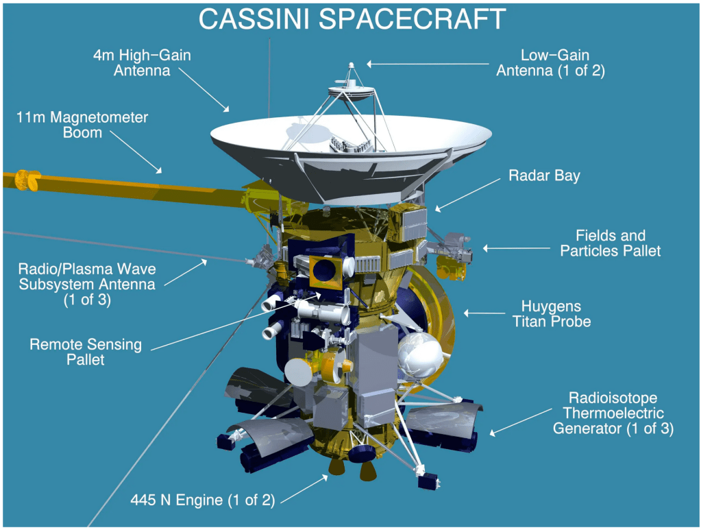
Scientists have been studying data from the Cassini spacecraft that observed Saturn close-up for over a decade from 2004 to 2017. Enceladus has a subsurface liquid ocean that generates plumes of tiny ice crystals that erupt like geysers from fissures in the solid surface. The ocean remains liquid because of internal tidal heating caused by the large gravitational forces of Saturn.
The Cassini spacecraft flew through the plumes and analyzed their content using its Cosmic Dust Analyzer. While the ice crystals from Enceladus were already known to contain organic compounds, the science team discovered that they also contain phosphorous. This is the least abundant element within the molecules of life, but it is absolutely essential, providing the backbone chemistry of DNA as well as being a constituent of amino acids.
With this discovery, all the essential building blocks of life are known to exist on Enceladus, along with a liquid ocean that is likely to be in chemical contact with rocky minerals on the ocean floor, possibly providing the kind of environment that could promote the emergence of life on a planet other than Earth.
Simulating the Expanding Universe in a Bose-Einstein Condensate
Putting the universe under a microscope in a laboratory may have seemed a foolish dream, until a group at the University of Heidelberg did just that. It isn’t possible to make a real universe in the laboratory, but by adjusting the properties of an ultra-cold collection of atoms known as a Bose-Einstein condensate, the research group was able to create a type of local space whose internal metric has a curvature, like curved space-time. Furthermore, by controlling the inter-atomic interactions of the condensate with a magnetic field, they could cause the condensate to expand or contract, mimicking different scenarios for the evolution of our own universe. By adjusting the type of expansion that occurs, the scientists could create hypotheses about the geometry of the universe and test them experimentally, something that could never be done in our own universe. This could lead to new insights into the behavior of the early universe and the formation of its large-scale structure.
This is the only breakthrough I picked that is not related to astrophysics (although even this effect may have played a role in the very early universe).
Entanglement is one of the hottest topics in physics today (although the idea is 89 years old) because of the crucial role it plays in quantum information physics. The topic was awarded the 2022 Nobel Prize in Physics which went to John Clauser, Alain Aspect and Anton Zeilinger.
Direct observations of entanglement have been mostly restricted to optics (where entangled photons are easily created and detected) or molecular and atomic physics as well as in the solid state.
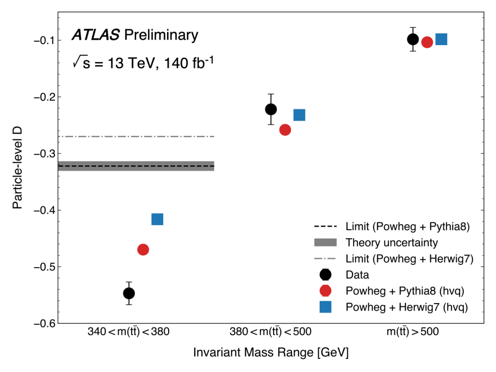
But entanglement eluded high-energy physics (which is quantum matter personified) until 2023 when the Atlas Collaboration at the LHC (Large Hadron Collider) in Geneva posted a manuscript on Arxiv that reported the first observation of entanglement in the decay products of a quark.
Fig. Thresholds for entanglement detection in decays from top quarks. Imagecredit.
Quarks interact so strongly (literally through the strong force), that entangled quarks experience very rapid decoherence, and entanglement effects virtually disappear in their decay products. However, top quarks decay so rapidly, that their entanglement properties can be transferred to their decay products, producing measurable effects in the downstream detection. This is what the Atlas team detected.
While this discovery won’t make quantum computers any better, it does open up a new perspective on high-energy particle interactions, and may even have contributed to the properties of the primordial soup during the Big Bang.
It may be hard to get excited about nothing … unless nothing is the whole ball game.
The only way we can really know what is, is by knowing what isn’t. Nothing is the backdrop against which we measure something. Experimentalists spend almost as much time doing control experiments, where nothing happens (or nothing is supposed to happen) as they spend measuring a phenomenon itself, the something.
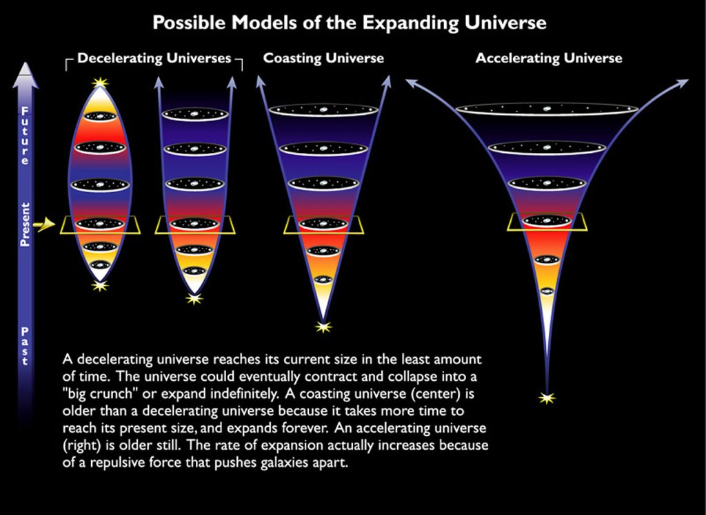
Even the universe, full of so much something, came out of nothing during the Big Bang. And today the energy density of nothing, so-called Dark Energy, is blowing our universe apart, propelling it ever faster to a bitter cold end.
So here is a brief history of nothing, tracing how we have understood what it is, where it came from, and where is it today.
With sturdy shoulders, space stands opposing all its weight to nothingness. Where space is, there is being.
Friedrich Nietzsche
40,000 BCE – Cosmic Origins
This is a human history, about how we homo sapiens try to understand the natural world around us, so the first step on a history of nothing is the Big Bang of human consciousness that occurred sometime between 100,000 – 40,000 years ago. Some sort of collective phase transition happened in our thought process when we seem to have become aware of our own existence within the natural world. This time frame coincides with the beginning of representational art and ritual burial. This is also likely the time when human language skills reached their modern form, and when logical arguments–stories–first were told to explain our existence and origins.
Roughly two origin stories emerged from this time. One of these assumes that what is has always been, either continuously or cyclically. Buddhism and Hinduism are part of this tradition as are many of the origin philosophies of Indigenous North Americans. Another assumes that there was a beginning when everything came out of nothing. Abrahamic faiths (Let there be light!) subscribe to this creatio ex nihilo. What came before creation? Nothing!
500 BCE – Leucippus and Democritus Atomism
The Greek philosopher Leucippus and his student Democritus, living around 500 BCE, were the first to lay out the atomic theory in which the elements of substance were indivisible atoms of matter, and between the atoms of matter was void. The different materials around us were created by the different ways that these atoms collide and cluster together. Plato later adhered to this theory, developing ideas along these lines in his Timeaus.
300 BCE – Aristotle Vacuum
Aristotle is famous for arguing, in his Physics Book IV, Section 8, that nature abhors a vacuum (horror vacui) because any void would be immediately filled by the imposing matter surrounding it. He also argued more philosophically that nothing, by definition, cannot exist.
1644 – Rene Descartes Vortex Theory
Fast forward a millennia and a half, and theories of existence were finally achieving a level of sophistication that can be called “scientific”. Rene Descartes followed Aristotle’s views of the vacuum, but he extended it to the vacuum of space, filling it with an incompressible fluid in his Principles of Philosophy (1644). Just like water, laminar motion can only occur by shear, leading to vortices. Descartes was a better philosopher than mathematician, so it took Christian Huygens to apply mathematics to vortex motion to “explain” the gravitational effects of the solar system.
Otto von Guericke is one of those hidden gems of the history of science, a person who almost no-one remembers today, but who was far in advance of his own day. He was a powerful politician, holding the position of Burgomeister of the city of Magdeburg for more than 30 years, helping to rebuild it after it was sacked during the Thirty Years War. He was also a diplomat, playing a key role in the reorientation of power within the Holy Roman Empire. How he had free time is anyone’s guess, but he used it to pursue scientific interests that spanned from electrostatics to his invention of the vacuum pump.
With a succession of vacuum pumps, each better than the last, von Geuricke was like a kid in a toy factory, pumping the air out of anything he could find. In the process, he showed that a vacuum would extinguish a flame and could raise water in a tube.
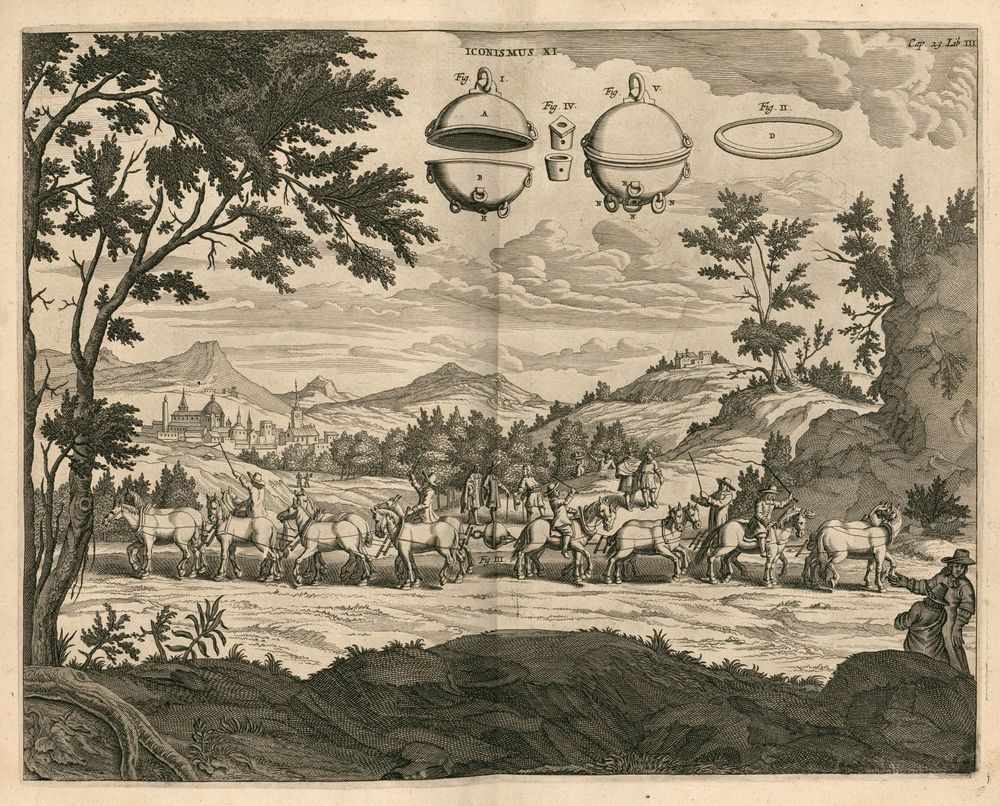
His most famous demonstration was, of course, the Magdeburg sphere demonstration. In 1657 he fabricated two 20-inch hemispheres that he attached together with a vacuum seal and used his vacuum pump to evacuate the air from inside. He then attached chains from the hemispheres to a team of eight horses on each side, for a total of 16 horses, who were unable to separate the spheres. This dramatically demonstrated that air exerts a force on surfaces, and that Aristotle and Descartes were wrong—nature did allow a vacuum!
1667 – Isaac Newton Action at a Distance
When it came to the vacuum, Newton was agnostic. His universal theory of gravitation posited action at a distance, but the intervening medium played no direct role.
Nothing comes from nothing, Nothing ever could.
Rogers and Hammerstein, The Sound of Music
This would seem to say that Newton had nothing to say about the vacuum, but his other major work, his Optiks, established particles as the elements of light rays. Such light particles travelled easily through vacuum, so the particle theory of light came down on the empty side of space.
Statue of Isaac Newton by Sir Eduardo Paolozzi based on a painting by William Blake. Image Credit
1821 – Augustin Fresnel Luminiferous Aether
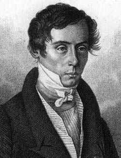
Today, we tend to think of Thomas Young as the chief proponent for the wave nature of light, going against the towering reputation of his own countryman Newton, and his courage and insights are admirable. But it was Augustin Fresnel who put mathematics to the theory. It was also Fresnel, working with his friend Francois Arago, who established that light waves are purely transverse.
For these contributions, Fresnel stands as one of the greatest physicists of the 1800’s. But his transverse light waves gave birth to one of the greatest red herrings of that century—the luminiferous aether. The argument went something like this, “if light is waves, then just as sound is oscillations of air, light must be oscillations of some medium that supports it – the luminiferous aether.” Arago searched for effects of this aether in his astronomical observations, but he didn’t see it, and Fresnel developed a theory of “partial aether drag” to account for Arago’s null measurement. Hippolyte Fizeau later confirmed the Fresnel “drag coefficient” in his famous measurement of the speed of light in moving water. (For the full story of Arago, Fresnel and Fizeau, see Chapter 2 of “Interference”. [1])
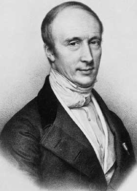
But the transverse character of light also required that this unknown medium must have some stiffness to it, like solids that support transverse elastic waves. This launched almost a century of alternative ideas of the aether that drew in such stellar actors as George Green, George Stokes and Augustin Cauchy with theories spanning from complete aether drag to zero aether drag with Fresnel’s partial aether drag somewhere in the middle.
1849 – Michael Faraday Field Theory
Micheal Faraday was one of the most intuitive physicists of the 1800’s. He worked by feel and mental images rather than by equations and proofs. He took nothing for granted, able to see what his experiments were telling him instead of looking only for what he expected.
This talent allowed him to see lines of force when he mapped out the magnetic field around a current-carrying wire. Physicists before him, including Ampere who developed a mathematical theory for the magnetic effects of a wire, thought only in terms of Newton’s action at a distance. All forces were central forces that acted in straight lines. Faraday’s experiments told him something different. The magnetic lines of force were circular, not straight. And they filled space. This realization led him to formulate his theory for the magnetic field.
Others at the time rejected this view, until William Thomson (the future Lord Kelvin) wrote a letter to Faraday in 1845 telling him that he had developed a mathematical theory for the field. He suggested that Faraday look for effects of fields on light, which Faraday found just one month later when he observed the rotation of the polarization of light when it propagated in a high-index material subject to a high magnetic field. This effect is now called Faraday Rotation and was one of the first experimental verifications of the direct effects of fields.
Nothing is more real than nothing.
Samuel Beckett
In 1949, Faraday stated his theory of fields in their strongest form, suggesting that fields in empty space were the repository of magnetic phenomena rather than magnets themselves [2]. He also proposed a theory of light in which the electric and magnetic fields induced each other in repeated succession without the need for a luminiferous aether.
1861 – James Clerk Maxwell Equations of Electromagnetism
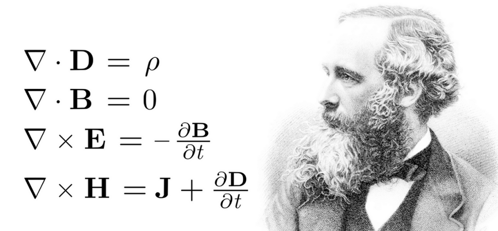
James Clerk Maxwell pulled the various electric and magnetic phenomena together into a single grand theory, although the four succinct “Maxwell Equations” was condensed by Oliver Heaviside from Maxwell’s original 15 equations (written using Hamilton’s awkward quaternions) down to the 4 vector equations that we know and love today.
One of the most significant and most surprising thing to come out of Maxwell’s equations was the speed of electromagnetic waves that matched closely with the known speed of light, providing near certain proof that light was electromagnetic waves.
However, the propagation of electromagnetic waves in Maxwell’s theory did not rule out the existence of a supporting medium—the luminiferous aether. It was still not clear that fields could exist in a pure vacuum but might still be like the stress fields in solids.
Late in his life, just before he died, Maxwell pointed out that no measurement of relative speed through the aether performed on a moving Earth could see deviations that were linear in the speed of the Earth but instead would be second order. He considered that such second-order effects would be far to small ever to detect, but Albert Michelson had different ideas.
1887 – Albert Michelson Null Experiment
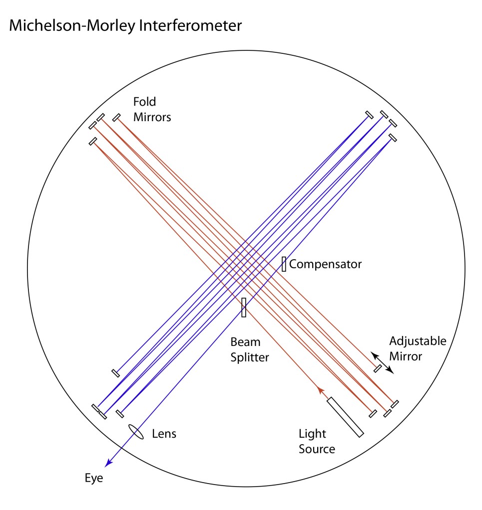
Albert Michelson was convinced of the existence of the luminiferous aether, and he was equally convinced that he could detect it. In 1880, working in the basement of the Potsdam Observatory outside Berlin, he operated his first interferometer in a search for evidence of the motion of the Earth through the aether. He had built the interferometer, what has come to be called a Michelson Interferometer, months earlier in the laboratory of Hermann von Helmholtz in the center of Berlin, but the footfalls of the horse carriages outside the building disturbed the measurements too much—Postdam was quieter.
But he could find no difference in his interference fringes as he oriented the arms of his interferometer parallel and orthogonal to the Earth’s motion. A simple calculation told him that his interferometer design should have been able to detect it—just barely—so the null experiment was a puzzle.
Seven years later, again in a basement (this time in a student dormitory at Western Reserve College in Cleveland, Ohio), Michelson repeated the experiment with an interferometer that was ten times more sensitive. He did this in collaboration with Edward Morley. But again, the results were null. There was no difference in the interference fringes regardless of which way he oriented his interferometer. Motion through the aether was undetectable.
(Michelson has a fascinating backstory, complete with firestorms (literally) and the Wild West and a moment when he was almost committed to an insane asylum against his will by a vengeful wife. To read all about this, see Chapter 4: After the Gold Rush in my recent book Interference (Oxford, 2023)).
The Michelson Morley experiment did not create the crisis in physics that it is sometimes credited with. They published their results, and the physics world took it in stride. Voigt and Fitzgerald and Lorentz and Poincaré toyed with various ideas to explain it away, but there had already been so many different models, from complete drag to no drag, that a few more theories just added to the bunch.
But they all had their heads in a haze. It took an unknown patent clerk in Switzerland to blow away the wisps and bring the problem into the crystal clear.
1905 – Albert Einstein Relativity
So much has been written about Albert Einstein’s “miracle year” of 1905 that it has lapsed into a form of physics mythology. Looking back, it seems like his own personal Big Bang, springing forth out of the vacuum. He published 5 papers that year, each one launching a new approach to physics on a bewildering breadth of problems from statistical mechanics to quantum physics, from electromagnetism to light … and of course, Special Relativity [3].
Whereas the others, Voigt and Fitzgerald and Lorentz and Poincaré, were trying to reconcile measurements of the speed of light in relative motion, Einstein just replaced all that musing with a simple postulate, his second postulate of relativity theory:
2. Any ray of light moves in the “stationary” system of co-ordinates with the determined velocity c, whether the ray be emitted by a stationary or by a moving body. Hence …
Albert Einstein, Annalen der Physik, 1905
And the rest was just simple algebra—in complete agreement with Michelson’s null experiment, and with Fizeau’s measurement of the so-called Fresnel drag coefficient, while also leading to the famous E = mc2 and beyond.
There is no aether. Electromagnetic waves are self-supporting in vacuum—changing electric fields induce changing magnetic fields that induce, in turn, changing electric fields—and so it goes.
The vacuum is vacuum—nothing! Except that it isn’t. It is still full of things.
1931 – P. A. M Dirac Antimatter
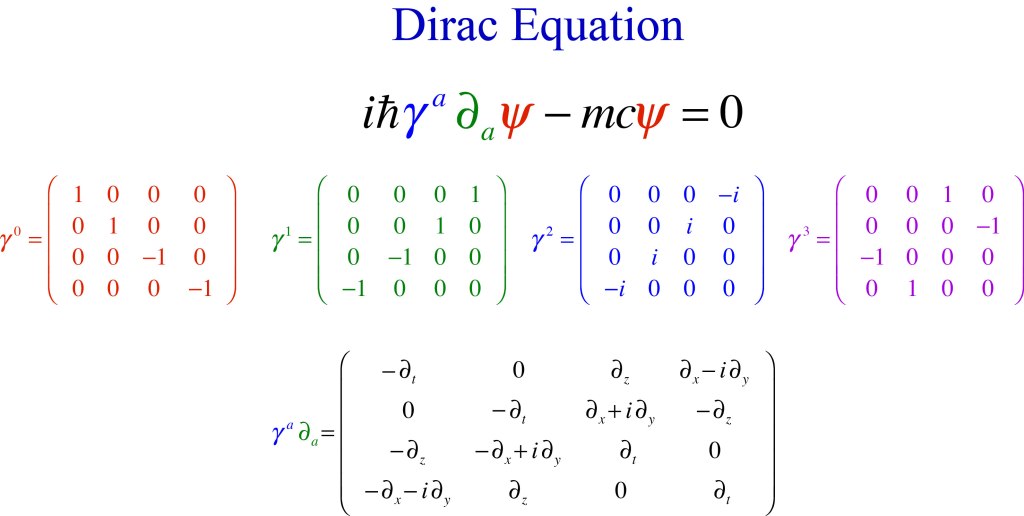
The Dirac equation is the famous end-product of P. A. M. Dirac’s search for a relativistic form of the Schrödinger equation. It replaces the asymmetric use in Schrödinger’s form of a second spatial derivative and a first time derivative with Dirac’s form using only first derivatives that are compatible with relativistic transformations [4].
One of the immediate consequences of this equation is a solution that has negative energy. At first puzzling and hard to interpret [5], Dirac eventually hit on the amazing proposal that these negative energy states are real particles paired with ordinary particles. For instance, the negative energy state associated with the electron was an anti-electron, a particle with the same mass as the electron, but with positive charge. Furthermore, because the anti-electron has negative energy and the electron has positive energy, these two particles can annihilate and convert their mass energy into the energy of gamma rays. This audacious proposal was confirmed by the American physicist Carl Anderson who discovered the positron in 1932.
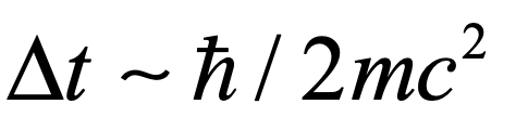
The existence of particles and anti-particles, combined with Heisenberg’s uncertainty principle, suggests that vacuum fluctuations can spontaneously produce electron-positron pairs that would then annihilate within a time related to the mass energy
Although this is an exceedingly short time (about 10-21 seconds), it means that the vacuum is not empty, but contains a frothing sea of particle-antiparticle pairs popping into and out of existence.
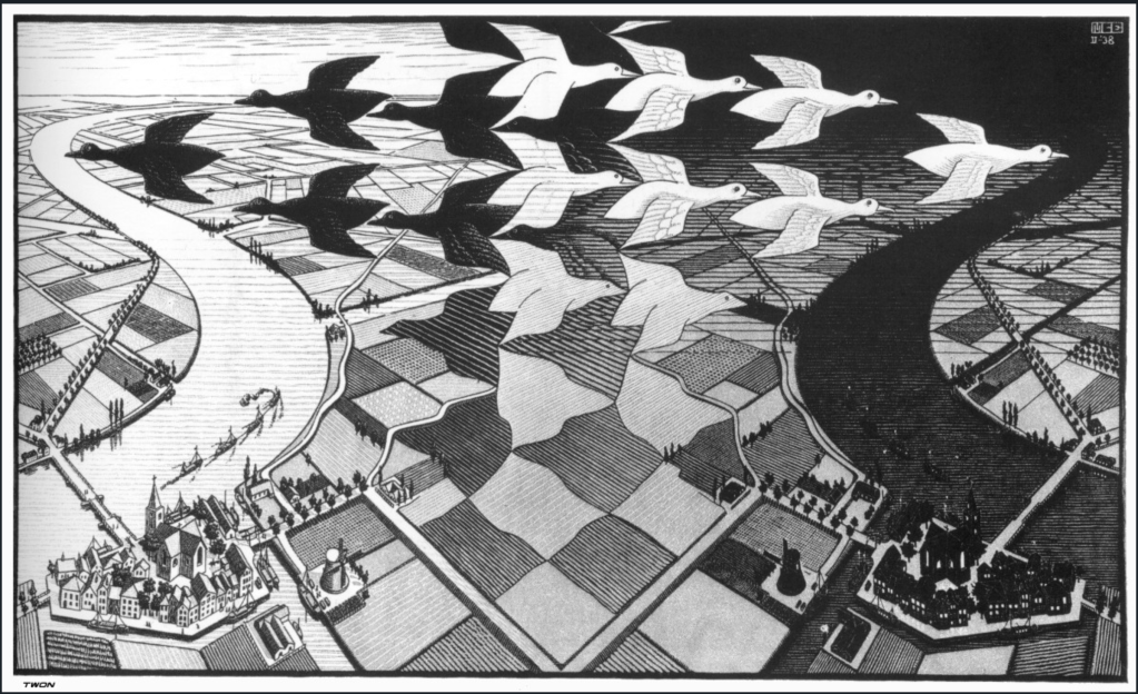
1938 – M. C. Escher Negative Space
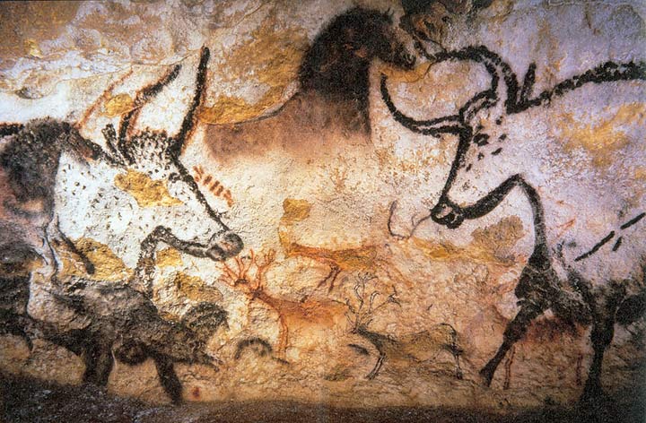
Scientists are not the only ones who think about empty space. Artists, too, are deeply committed to a visual understanding of our world around us, and the uses of negative space in art dates back virtually to the first cave paintings. However, artists and art historians only talked explicitly in such terms since the 1930’s and 1940’s [6]. One of the best early examples of the interplay between positive and negative space was a print made by M. C. Escher in 1938 titled “Day and Night”.
1946 – Edward Purcell Modified Spontaneous Emission
In 1916 Einstein laid out the laws of photon emission and absorption using very simple arguments (his modus operandi) based on the principles of detailed balance. He discovered that light can be emitted either spontaneously or through stimulated emission (the basis of the laser) [7]. Once the nature of vacuum fluctuations was realized through the work of Dirac, spontaneous emission was understood more deeply as a form of stimulated emission caused by vacuum fluctuations. In the absence of vacuum fluctuations, spontaneous emission would be inhibited. Conversely, if vacuum fluctuations are enhanced, then spontaneous emission would be enhanced.
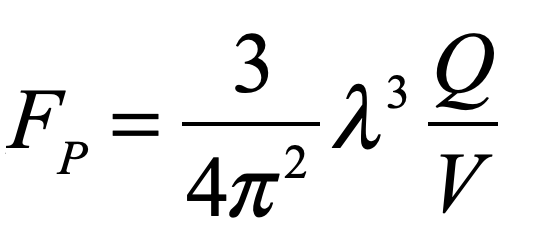
This effect was observed by Edward Purcell in 1946 through the observation of emission times of an atom in a RF cavity [8]. When the atomic transition was resonant with the cavity, spontaneous emission times were much faster. The Purcell enhancement factor is
where Q is the “Q” of the cavity, and V is the cavity volume. The physical basis of this effect is the modification of vacuum fluctuations by the cavity modes caused by interference effects. When cavity modes have constructive interference, then vacuum fluctuations are larger, and spontaneous emission is stimulated more quickly.
1948 – Hendrik Casimir Vacuum Force
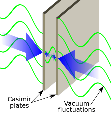
Interference effects in a cavity affect the total energy of the system by excluding some modes which become inaccessible to vacuum fluctuations. This lowers the internal energy internal to a cavity relative to free space outside the cavity, resulting in a net “pressure” acting on the cavity. If two parallel plates are placed in close proximity, this would cause a force of attraction between them. The effect was predicted in 1948 by Hendrik Casimir [9], but it was not verified experimentally until 1997 by S. Lamoreaux at Yale University [10].
Two plates brought very close feel a pressure exerted by the higher vacuum energy density external to the cavity.
1949 – Shinichiro Tomonaga, Richard Feynman and Julian Schwinger QED
The physics of the vacuum in the years up to 1948 had been a hodge-podge of ad hoc theories that captured the qualitative aspects, and even some of the quantitative aspects of vacuum fluctuations, but a consistent theory was lacking until the work of Tomonaga in Japan, Feynman at Cornell and Schwinger at Harvard. Feynman and Schwinger both published their theory of quantum electrodynamics (QED) in 1949. They were actually scooped by Tomonaga, who had developed his theory earlier during WWII, but physics research in Japan had been cut off from the outside world. It was when Oppenheimer received a letter from Tomonaga in 1949 that the West became aware of his work. All three received the Nobel Prize for their work on QED in 1965. Precision tests of QED now make it one of the most accurately confirmed theories in physics.
Richard Feynman’s first “Feynman diagram”.
1964 – Peter Higgs and The Higgs
The Higgs particle, known as “The Higgs”, was the brain-child of Peter Higgs, Francois Englert and Gerald Guralnik in 1964. Higgs’ name became associated with the theory because of a response letter he wrote to an objection made about the theory. The Higg’s mechanism is spontaneous symmetry breaking in which a high-symmetry potential can lower its energy by distorting the field, arriving at a new minimum in the potential. This mechanism can allow the bosons that carry force to acquire mass (something the earlier Yang-Mills theory could not do).
Spontaneous symmetry breaking is a ubiquitous phenomenon in physics. It occurs in the solid state when crystals can lower their total energy by slightly distorting from a high symmetry to a low symmetry. It occurs in superconductors in the formation of Cooper pairs that carry supercurrents. And here it occurs in the Higgs field as the mechanism to imbues particles with mass .
Conceptual graph of a potential surface where the high symmetry potential is higher than when space is distorted to lower symmetry. Image Credit
The theory was mostly ignored for its first decade, but later became the core of theories of electroweak unification. The Large Hadron Collider (LHC) at Geneva was built to detect the boson, announced in 2012. Peter Higgs and Francois Englert were awarded the Nobel Prize in Physics in 2013, just one year after the discovery.
The Higgs field permeates all space, and distortions in this field around idealized massless point particles are observed as mass. In this way empty space becomes anything but.
1981 – Alan Guth Inflationary Big Bang
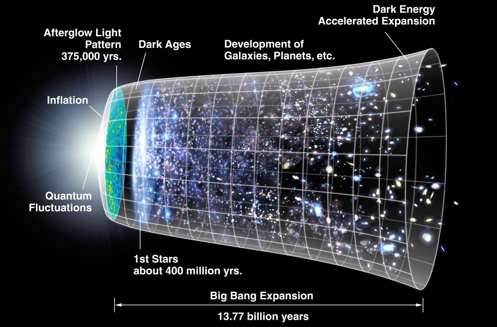
Problems arose in observational cosmology in the 1970’s when it was understood that parts of the observable universe that should have been causally disconnected were in thermal equilibrium. This could only be possible if the universe were much smaller near the very beginning. In January of 1981, Alan Guth, then at Cornell University, realized that a rapid expansion from an initial quantum fluctuation could be achieved if an initial “false vacuum” existed in a positive energy density state (negative vacuum pressure). Such a false vacuum could relax to the ordinary vacuum, causing a period of very rapid growth that Guth called “inflation”. Equilibrium would have been achieved prior to inflation, solving the observational problem.Therefore, the inflationary model posits a multiplicities of different types of “vacuum”, and once again, simple vacuum is not so simple.
Energy density as a function of a scalar variable. Quantum fluctuations create a “false vacuum” that can relax to “normal vacuum: by expanding rapidly. Image Credit
1998 – Saul Pearlmutter Dark Energy
Einstein didn’t make many mistakes, but in the early days of General Relativity he constructed a theoretical model of a “static” universe. A central parameter in Einstein’s model was something called the Cosmological Constant. By tuning it to balance gravitational collapse, he tuned the universe into a static Ithough unstable) state. But when Edwin Hubble showed that the universe was expanding, Einstein was proven incorrect. His Cosmological Constant was set to zero and was considered to be a rare blunder.
Fast forward to 1999, and the Supernova Cosmology Project, directed by Saul Pearlmutter, discovered that the expansion of the universe was accelerating. The simplest explanation was that Einstein had been right all along, or at least partially right, in that there was a non-zero Cosmological Constant. Not only is the universe not static, but it is literally blowing up. The physical origin of the Cosmological Constant is believed to be a form of energy density associated with the space of the universe. This “extra” energy density has been called “Dark Energy”, filling empty space.
The bottom line is that nothing, i.e., the vacuum, is far from nothing. It is filled with a froth of particles, and energy, and fields, and potentials, and broken symmetries, and negative pressures, and who knows what else as modern physics has been much ado about this so-called nothing, almost more than it has been about everything else.
[2] L. Peirce Williams in “Faraday, Michael.” Complete Dictionary of Scientific Biography, vol. 4, Charles Scribner’s Sons, 2008, pp. 527-540.
[3] A. Einstein, “On the electrodynamics of moving bodies,” Annalen Der Physik 17, 891-921 (1905).
[4] Dirac, P. A. M. (1928). “The Quantum Theory of the Electron”. Proceedings of the Royal Society A: Mathematical, Physical and Engineering Sciences. 117 (778): 610–624.
[5] Dirac, P. A. M. (1930). “A Theory of Electrons and Protons”. Proceedings of the Royal Society A: Mathematical, Physical and Engineering Sciences. 126 (801): 360–365.
[6] Nikolai M Kasak, Physical Art: Action of positive and negative space, (Rome, 1947/48) [2d part rev. in 1955 and 1956].
[7] A. Einstein, “Strahlungs-Emission un -Absorption nach der Quantentheorie,” Verh. Deutsch. Phys. Ges. 18, 318 (1916).
[8] Purcell, E. M. (1946-06-01). “Proceedings of the American Physical Society: Spontaneous Emission Probabilities at Ratio Frequencies”. Physical Review. American Physical Society (APS). 69 (11–12): 681.
[9] Casimir, H. B. G. (1948). “On the attraction between two perfectly conducting plates”. Proc. Kon. Ned. Akad. Wet. 51: 793.
[10] Lamoreaux, S. K. (1997). “Demonstration of the Casimir Force in the 0.6 to 6 μm Range”. Physical Review Letters. 78 (1): 5–8.
Read more in Books by David Nolte at Oxford University Press
Light is one of the most powerful manifestations of the forces of physics because it tells us about our reality. The interference of light, in particular, has led to the detection of exoplanets orbiting distant stars, discovery of the first gravitational waves, capture of images of black holes and much more. The stories behind the history of light and interference go to the heart of how scientists do what they do and what they often have to overcome to do it. These time-lines are organized along the chapter titles of the book Interference. They follow the path of theories of light from the first wave-particle debate, through the personal firestorms of Albert Michelson, to the discoveries of the present day in quantum information sciences.
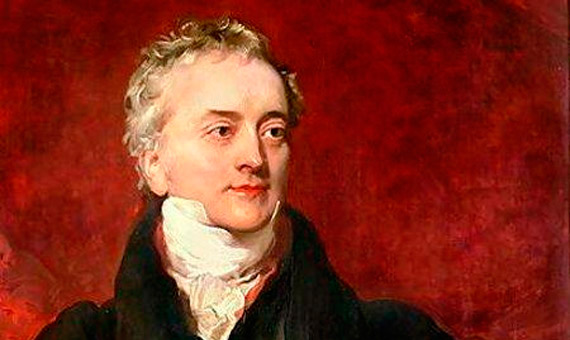
Thomas Young was the ultimate dabbler, his interests and explorations ranged far and wide, from ancient egyptology to naval engineering, from physiology of perception to the physics of sound and light. Yet unlike most dabblers who accomplish little, he made original and seminal contributions to all these fields. Some have called him the “Last Man Who Knew Everything“.
Thomas Young. The Law of Interference.
Topics: The Law of Interference. The Rosetta Stone. Benjamin Thompson, Count Rumford. Royal Society. Christiaan Huygens. Pendulum Clocks. Icelandic Spar. Huygens’ Principle. Stellar Aberration. Speed of Light. Double-slit Experiment.
1629 – Huygens born (1629 – 1695)
1642 – Galileo dies, Newton born (1642 – 1727)
1655 – Huygens ring of Saturn
1657 – Huygens patents the pendulum clock
1666 – Newton prismatic colors
1666 – Huygens moves to Paris
1669 – Bartholin double refraction in Icelandic spar
1670 – Bartholinus polarization of light by crystals
1671 – Expedition to Hven by Picard and Rømer
1673 – James Gregory bird-feather diffraction grating
1801 – Young Theory of Light and Colours, three color mechanism (Bakerian Lecture), Young considers interference to cause the colored films, first estimates of the wavelengths of different colors
1802 – Young begins series of lecturs at the Royal Institution (Jan. 1802 – July 1803)
1802 – Young names the principle (Law) of interference
Augustin Fresnel was an intuitive genius whose talents were almost squandered on his job building roads and bridges in the backwaters of France until he was discovered and rescued by Francois Arago.
Topics: Particles versus Waves. Malus and Polarization. Agustin Fresnel. Francois Arago. Diffraction. Daniel Bernoulli. The Principle of Superposition. Joseph Fourier. Transverse Light Waves.
1665 – Grimaldi diffraction bands outside shadow
1673 – James Gregory bird-feather diffraction grating
There is no question that Francois Arago was a swashbuckler. His life’s story reads like an adventure novel as he went from being marooned in hostile lands early in his career to becoming prime minister of France after the 1848 revolutions swept across Europe.
Topics: The Birth of Interferometry. Snell’s Law. Fresnel and Arago. The First Interferometer. Fizeau and Foucault. The Speed of Light. Ether Drag. Jamin Interferometer.
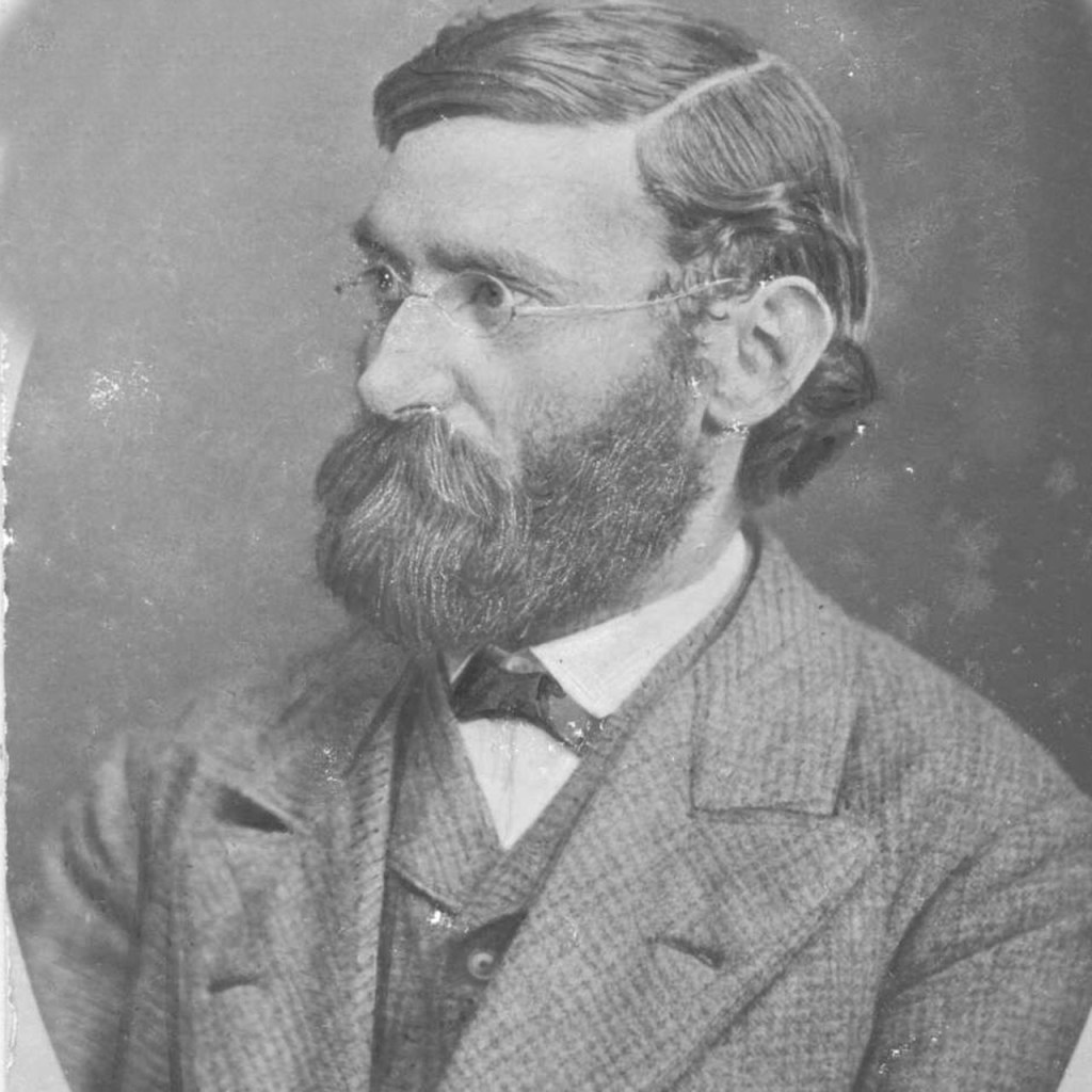
No name is more closely connected to interferometry than that of Albert Michelson. He succeeded, sometimes at great personal cost, in launching interferometric metrology as one of the most important tools used by scientists today.
Albert A. Michelson, 1907 Nobel Prize. Image Credit.
Topics: The Trials of Albert Michelson. Hermann von Helmholtz. Michelson and Morley. Fabry and Perot.
1810 – Arago search for ether drag
1813 – Fraunhofer dark lines in Sun spectrum
1813 – Faraday begins at Royal Institution
1820 – Oersted discovers electromagnetism
1821 – Faraday electromagnetic phenomena
1827 – Green mathematical analysis of electricity and magnetism
1830 – Cauchy ether as elastic solid
1831 – Faraday electromagnetic induction
1831 – Cauchy ether drag
1831 – Maxwell born
1831 – Faraday electromagnetic induction
1836 – Cauchy’s second theory of the ether
1838 – Green theory of the ether
1839 – Hamilton group velocity
1839 – MacCullagh properties of rotational ether
1839 – Cauchy ether with negative compressibility
1841 – Maxwell entered Edinburgh Academy (age 10) met P. G. Tait
1842 – Doppler effect
1845 – Faraday effect (magneto-optic rotation)
1846 – Stokes’ viscoelastic theory of the ether
1847 – Maxwell entered Edinburgh University
1850 – Maxwell at Cambridge, studied under Hopkins, also knew Stokes and Whewell
1852 – Michelson born Strelno, Prussia
1854 – Maxwell wins the Smith’s Prize (Stokes’ theorem was one of the problems)
1855 – Michelson’s immigrate to San Francisco through Panama Canal
Learning from his attempts to measure the speed of light through the ether, Michelson realized that the partial coherence of light from astronomical sources could be used to measure their sizes. His first measurements using the Michelson Stellar Interferometer launched a major subfield of astronomy that is one of the most active today.
R Hanbury Brown
Topics: Measuring the Stars. Astrometry. Moons of Jupiter. Schwarzschild. Betelgeuse. Michelson Stellar Interferometer. Banbury Brown Twiss. Sirius. Adaptive Optics.
1838 – Bessel stellar parallax measurement with Fraunhofer telescope
1868 – Fizeau proposes stellar interferometry
1873 – Stephan implements Fizeau’s stellar interferometer on Sirius, sees fringes
1880 – Michelson Idea for second-order measurement of relative motion against ether
1880 – 1882 Michelson Studies in Europe (Helmholtz in Berlin, Quincke in Heidelberg, Cornu, Mascart and Lippman in Paris)
1881 – Michelson Measurement at Potsdam with funds from Alexander Graham Bell
1881 – Michelson Resigned from active duty in the Navy
1883 – Michelson Joined Case School of Applied Science
1889 – Michelson moved to Clark University at Worcester
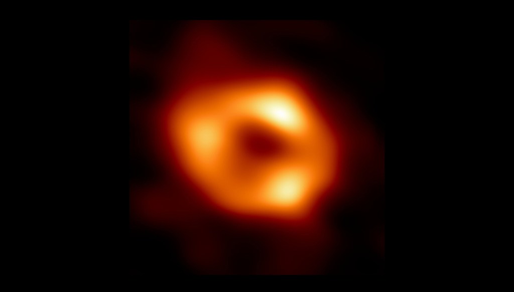
Stellar interferometry is opening new vistas of astronomy, exploring the wildest occupants of our universe, from colliding black holes half-way across the universe (LIGO) to images of neighboring black holes (EHT) to exoplanets near Earth that may harbor life.
Image of the supermassive black hole in M87 from Event Horizon Telescope.
Topics: Gravitational Waves, Black Holes and the Search for Exoplanets. Nulling Interferometer. Event Horizon Telescope. M87 Black Hole. Long Baseline Interferometry. LIGO.
1947 – Virgo A radio source identified as M87
1953 – Horace W. Babcock proposes adaptive optics (AO)
From the astronomically large dimensions of outer space to the microscopically small dimensions of inner space, optical interference pushes the resolution limits of imaging.
Topics: Diffraction and Interference. Joseph Fraunhofer. Diffraction Gratings. Henry Rowland. Carl Zeiss. Ernst Abbe. Phase-contrast Microscopy. Super-resolution Micrscopes. Structured Illumination.
The coherence of laser light is like a brilliant jewel that sparkles in the darkness, illuminating life, probing science and projecting holograms in virtual worlds.
What is the image of one photon interfering? Better yet, what is the image of two photons interfering? The answer to this crucial question laid the foundation for quantum communication.
Topics: The Beginnings of Quantum Communication. EPR paradox. Entanglement. David Bohm. John Bell. The Bell Inequalities. Leonard Mandel. Single-photon Interferometry. HOM Interferometer. Two-photon Fringes. Quantum cryptography. Quantum Teleportation.
1900 – Planck (1901). “Law of energy distribution in normal spectra.” [1]
There is almost no technical advantage better than having exponential resources at hand. The exponential resources of quantum interference provide that advantage to quantum computing which is poised to usher in a new era of quantum information science and technology.
David Deutsch.
Topics: Interferometric Computing. David Deutsch. Quantum Algorithm. Peter Shor. Prime Factorization. Quantum Logic Gates. Linear Optical Quantum Computing. Boson Sampling. Quantum Computational Advantage.
1980 – Paul Benioff describes possibility of quantum computer
[10] B. R. Mollow, R. J. Glauber: Phys. Rev. 160, 1097 (1967); 162, 1256 (1967)
[11] J. F. Clauser, M. A. Horne, A. Shimony, and R. A. Holt, ” Proposed experiment to test local hidden-variable theories,” Physical Review Letters, vol. 23, no. 15, pp. 880-&, (1969)
[15] R. Ghosh and L. Mandel, “Observation of nonclassical effects in the interference of 2 photons,” Physical Review Letters, vol. 59, no. 17, pp. 1903-1905, Oct (1987)
[16] C. K. Hong, Z. Y. Ou, and L. Mandel, “Measurement of subpicosecond time intervals between 2 photons by interference,” Physical Review Letters, vol. 59, no. 18, pp. 2044-2046, Nov (1987)
[18] D. Deutsch, “QUANTUM-THEORY, THE CHURCH-TURING PRINCIPLE AND THE UNIVERSAL QUANTUM COMPUTER,” Proceedings of the Royal Society of London Series a-Mathematical Physical and Engineering Sciences, vol. 400, no. 1818, pp. 97-117, (1985)
[19] P. W. Shor, “ALGORITHMS FOR QUANTUM COMPUTATION – DISCRETE LOGARITHMS AND FACTORING,” in 35th Annual Symposium on Foundations of Computer Science, Proceedings, S. Goldwasser Ed., (Annual Symposium on Foundations of Computer Science, 1994, pp. 124-134.
[20] F. Arute et al., “Quantum supremacy using a programmable superconducting processor,” Nature, vol. 574, no. 7779, pp. 505-+, Oct 24 (2019)
[21] H.-S. Zhong et al., “Quantum computational advantage using photons,” Science, vol. 370, no. 6523, p. 1460, (2020)
Further Reading: The History of Light and Interference (2023)
The first step on the road to Einstein’s relativity was taken a hundred years earlier by an ironic rebel of physics—Augustin Fresnel. His radical (at the time) wave theory of light was so successful, especially the proof that it must be composed of transverse waves, that he was single-handedly responsible for creating the irksome luminiferous aether that would haunt physicists for the next century. It was only when Einstein combined the work of Fresnel with that of Hippolyte Fizeau that the aether was ultimately banished.
Augustin Fresnel: Ironic Rebel of Physics
Augustin Fresnel was an odd genius who struggled to find his place in the technical hierarchies of France. After graduating from the Ecole Polytechnique, Fresnel was assigned a mindless job overseeing the building of roads and bridges in the boondocks of France—work he hated. To keep himself from going mad, he toyed with physics in his spare time, and he stumbled on inconsistencies in Newton’s particulate theory of light that Laplace, a leader of the French scientific community, embraced as if it were revealed truth .
The final irony is that Einstein used Fresnel’s theoretical coefficient and Fizeau’s measurements—that had introduced aether drag in the first place—to show that there was no aether.
Fresnel rebelled, realizing that effects of diffraction could be explained if light were made of waves. He wrote up an initial outline of his new wave theory of light, but he could get no one to listen, until Francois Arago heard of it. Arago was having his own doubts about the particle theory of light based on his experiments on stellar aberration.
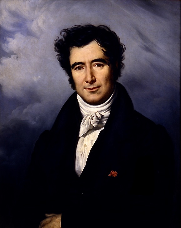
Augustin Fresnel and Francois Arago (circa 1818)
Stellar Aberration and the Fresnel Drag Coefficient
Stellar aberration had been explained by James Bradley in 1729 as the effect of the motion of the Earth relative to the motion of light “particles” coming from a star. The Earth’s motion made it look like the star was tilted at a very small angle (see my previous blog). That explanation had worked fine for nearly a hundred years, but then around 1810 Francois Arago at the Paris Observatory made extremely precise measurements of stellar aberration while placing finely ground glass prisms in front of his telescope. According to Snell’s law of refraction, which depended on the velocity of the light particles, the refraction angle should have been different at different times of the year when the Earth was moving one way or another relative to the speed of the light particles. But to high precision the effect was absent. Arago began to question the particle theory of light. When he heard about Fresnel’s work on the wave theory, he arranged a meeting, encouraging Fresnel to continue his work.
But at just this moment, in March of 1815, Napoleon returned from exile in Elba and began his march on Paris with a swelling army of soldiers who flocked to him. Fresnel rebelled again, joining a royalist militia to oppose Napoleon’s return. Napoleon won, but so did Fresnel, who was ironically placed under house arrest, which was like heaven to him. It freed him from building roads and bridges, giving him free time to do optics experiments in his mother’s house to support his growing theoretical work on the wave nature of light.
Arago convinced the authorities to allow Fresnel to come to Paris, where the two began experiments on diffraction and interference. By using polarizers to control the polarization of the interfering light paths, they concluded that light must be composed of transverse waves.
This brilliant insight was then followed by one of the great tragedies of science—waves needed a medium within which to propagate, so Fresnel conceived of the luminiferous aether to support it. Worse, the transverse properties of light required the aether to have a form of crystalline stiffness.
How could moving objects, like the Earth orbiting the sun, travel through such an aether without resistance? This was a serious problem for physics. One solution was that the aether was entrained by matter, so that as matter moved, the aether was dragged along with it. That solved the resistance problem, but it raised others, because it couldn’t explain Arago’s refraction measurements of aberration.
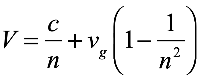
Fresnel realized that Arago’s null results could be explained if aether was only partially dragged along by matter. For instance, in the glass prisms used by Arago, the fraction of the aether being dragged along by the moving glass versus at rest would depend on the refractive index n of the glass. The speed of light in moving glass would then be
where c is the speed of light through stationary aether, vg is the speed of the glass prism through the stationary aether, and V is the speed of light in the moving glass. The first term in the expression is the ordinary definition of the speed of light in stationary matter with the refractive index. The second term is called the Fresnel drag coefficient which he communicated to Arago in a letter in 1818. Even at the high speed of the Earth moving around the sun, this second term is a correction of only about one part in ten thousand. It explained Arago’s null results for stellar aberration, but it was not possible to measure it directly in the laboratory at that time.
Fizeau’s Moving Water Experiment
Hippolyte Fizeau has the distinction of being the first to measure the speed of light directly in an Earth-bound experiment. All previous measurements had been astronomical. The story of his ingenious use of a chopper wheel and long-distance reflecting mirrors placed across the city of Paris in 1849 can be found in Chapter 3 of Interference. However, two years later he completed an experiment that few at the time noticed but which had a much more profound impact on the history of physics.
Hippolyte Fizeau
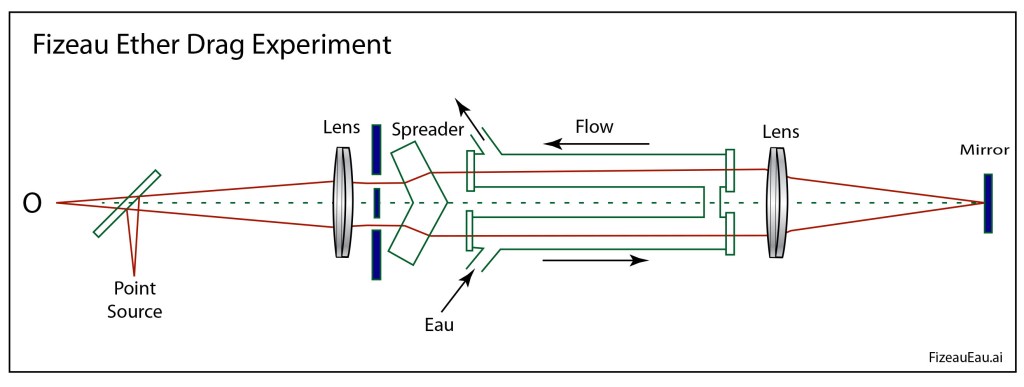
In 1851, Fizeau modified an Arago interferometer to pass two interfering light beams along pipes of moving water. The goal of the experiment was to measure the aether drag coefficient directly and to test Fresnel’s theory of partial aether drag. The interferometer allowed Fizeau to measure the speed of light in moving water relative to the speed of light in stationary water. The results of the experiment confirmed Fresnel’s drag coefficient to high accuracy, which seemed to confirm the partial drag of aether by moving matter.
Fizeau’s 1851 measurement of the speed of light in water using a modified Arago interferometer. (Reprinted from Chapter 2: Interference.)
This result stood for thirty years, presenting its own challenges for physicist exploring theories of the aether. The sophistication of interferometry improved over that time, and in 1881 Albert Michelson used his newly-invented interferometer to measure the speed of the Earth through the aether. He performed the experiment in the Potsdam Observatory outside Berlin, Germany, and found the opposite result of complete aether drag, contradicting Fizeau’s experiment. Later, after he began collaborating with Edwin Morley at Case and Western Reserve Colleges in Cleveland, Ohio, the two repeated Fizeau’s experiment to even better precision, finding once again Fresnel’s drag coefficient, followed by their own experiment, known now as “the Michelson-Morley Experiment” in 1887, that found no effect of the Earth’s movement through the aether.
The two experiments—Fizeau’s measurement of the Fresnel drag coefficient, and Michelson’s null measurement of the Earth’s motion—were in direct contradiction with each other. Based on the theory of the aether, they could not both be true.
But where to go from there? For the next 15 years, there were numerous attempts to put bandages on the aether theory, from Fitzgerald’s contraction to Lorenz’ transformations, but it all seemed like kludges built on top of kludges. None of it was elegant—until Einstein had his crucial insight.
Einstein’s Insight
While all the other top physicists at the time were trying to save the aether, taking its real existence as a fact of Nature to be reconciled with experiment, Einstein took the opposite approach—he assumed that the aether did not exist and began looking for what the experimental consequences would be.
From the days of Galileo, it was known that measured speeds depended on the frame of reference. This is why a knife dropped by a sailor climbing the mast of a moving ship strikes at the base of the mast, falling in a straight line in the sailor’s frame of reference, but an observer on the shore sees the knife making an arc—velocities of relative motion must add. But physicists had over-generalized this result and tried to apply it to light—Arago, Fresnel, Fizeau, Michelson, Lorenz—they were all locked in a mindset.
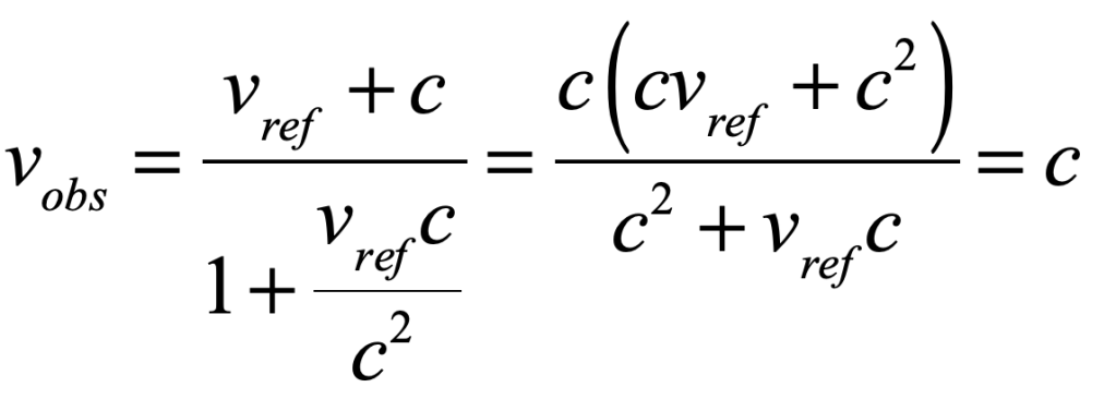
Einstein stepped outside that mindset and asked what would happen if all relatively moving observers measured the same value for the speed of light, regardless of their relative motion. It was just a little algebra to find that the way to add the speed of light c to the speed of a moving reference frame vref was
where the numerator was the usual Galilean relativity velocity addition, and the denominator was required to enforce the constancy of observed light speeds. Therefore, adding the speed of light to the speed of a moving reference frame gives back simply the speed of light.
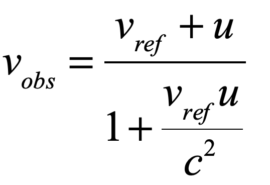
Generalizing this equation for general velocity addition between moving frames gives
where u is now the speed of some moving object being added the the speed of a reference frame, and vobs is the “net” speed observed by some “external” observer . This is Einstein’s famous equation for relativistic velocity addition (see pg. 12 of the English translation). It ensures that all observers with differently moving frames all measure the same speed of light, while also predicting that no velocities for objects can ever exceed the speed of light.
This last fact is a consequence, not an assumption, as can be seen by letting the reference speed vref increase towards the speed of light so that vref ≈ c, then
so that the speed of an object launched in the forward direction from a reference frame moving near the speed of light is still observed to be no faster than the speed of light
All of this, so far, is theoretical. Einstein then looked to find some experimental verification of his new theory of relativistic velocity addition, and he thought of the Fizeau experimental measurement of the speed of light in moving water. Applying his new velocity addition formula to the Fizeau experiment, he set vref = vwater and u = c/n and found
The second term in the denominator is much smaller that unity and is expanded in a Taylor’s expansion
The last line is exactly the Fresnel drag coefficient!
Therefore, Fizeau, half a century before, in 1851, had already provided experimental verification of Einstein’s new theory for relativistic velocity addition! It wasn’t aether drag at all—it was relativistic velocity addition.
From this point onward, Einstein followed consequence after inexorable consequence, constructing what is now called his theory of Special Relativity, complete with relativistic transformations of time and space and energy and matter—all following from a simple postulate of the constancy of the speed of light and the prescription for the addition of velocities.
The final irony is that Einstein used Fresnel’s theoretical coefficient and Fizeau’s measurements, that had established aether drag in the first place, as the proof he needed to show that there was no aether. It was all just how you looked at it.
• The history behind Einstein’s use of relativistic velocity addition is given in: A. Pais, Subtle is the Lord: The Science and the Life of Albert Einstein (Oxford University Press, 2005).
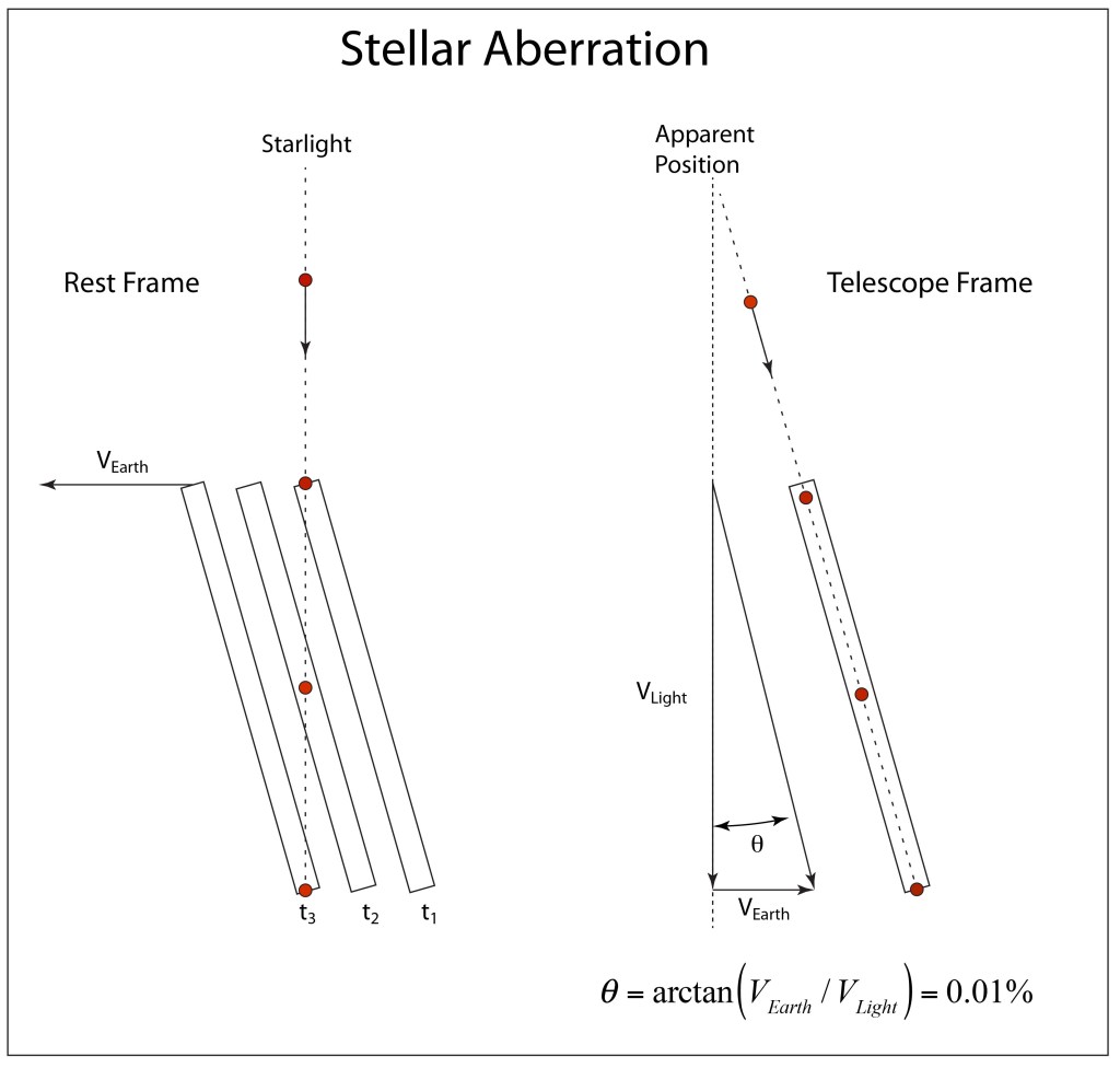
The Earth races around the sun with remarkable speed—at over one hundred thousand kilometers per hour on its yearly track. This is about 0.01% of the speed of light—a small but non-negligible amount for which careful measurement might show the very first evidence of relativistic effects. How big is this effect and how do you measure it? One answer is the aberration of starlight, which is the slight deviation in the apparent position of stars caused by the linear speed of the Earth around the sun.
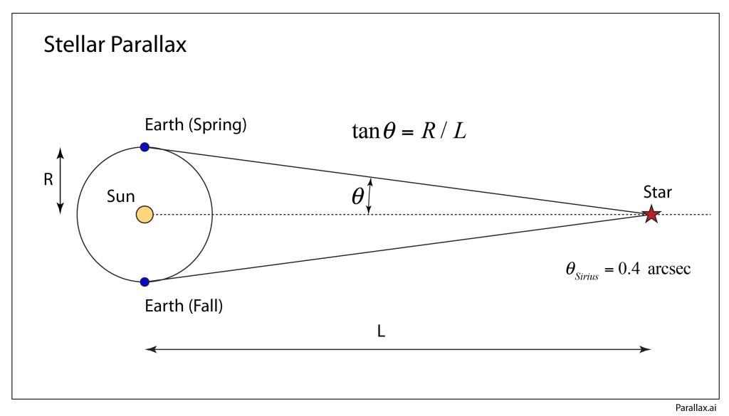
This is not parallax, which is caused the the changing position of the Earth around the sun. Ever since Copernicus, astronomers had been searching for parallax, which would give some indication how far away stars were. It was an important question, because the answer would say something about how big the universe was. But in the process of looking for parallax, astronomers found something else, something about 50 times bigger—aberration.
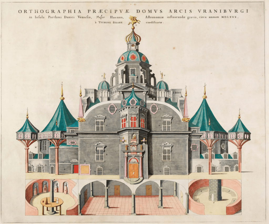
Aberration is the effect of the transverse speed of the Earth added to the speed of light coming from a star. For instance, this effect on the apparent location of stars in the sky is a simple calculation of the arctangent of 0.01%, which is an angle of about 20 seconds of arc, or about 40 seconds when comparing two angles 6 months apart. This was a bit bigger than the accuracy of astronomical measurements at the time when Jean Picard travelled from Paris to Denmark in 1671 to visit the ruins of the old observatory of Tycho Brahe at Uranibourg.
Fig. 1 Stellar parallax is the change in apparent positions of a star caused by the change in the Earth’s position as it orbits the sun. If the change in angle (θ) could be measured, then based on Newton’s theory of gravitation that gives the radius of the Earth’s orbit (R), the distance to the star (L) could be found.
Jean Picard at Uranibourg
Fig. 2 A view of Tycho Brahe’s Uranibourg astronomical observatory in Hven, Denmark. Tycho had to abandon it near the end of his life when a new king thought he was performing witchcraft.
Jean Picard went to Uranibourg originally in 1671, and during subsequent years, to measure the eclipses of the moons of Jupiter to determine longitude at sea—an idea first proposed by Galileo. When visiting Copenhagen, before heading out to the old observatory, Picard secured the services of an as yet unknown astronomer by the name of Ole Rømer. While at Uranibourg, Picard and Rømer made their required measurements of the eclipses of the moons of Jupiter, but with extra observation hours, Picard also made measurements of the positions of selected stars, such as Polaris, the North Star. His very precise measurements allowed him to track a tiny yearly shift, an aberration, in position by about 40 seconds of arc. At the time (before Rømer’s great insight about the finite speed of light—see Chapter 1 of Interference (Oxford, 2023)), the speed of light was thought to be either infinite or unmeasurably fast, so Picard thought that this shift was the long-sought effect of stellar parallax that would serve as a way to measure the distance to the stars. However, the direction of the shift of Polaris was completely wrong if it were caused by parallax, and Picard’s stellar aberration remained a mystery.
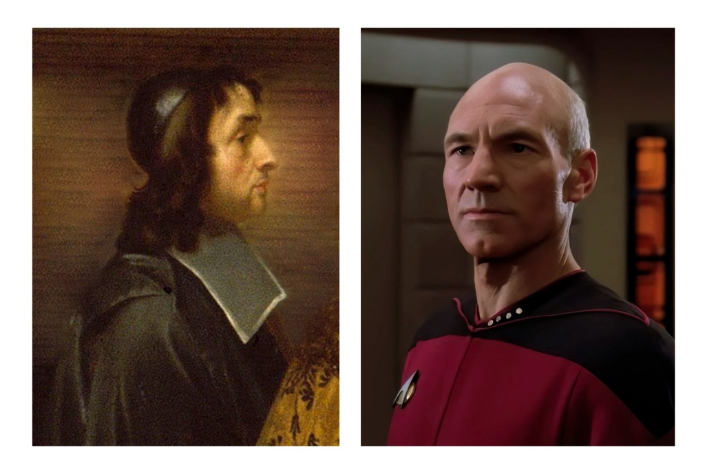
Fig. 3 Jean Picard (left) and his modern name-sake (right).
Samuel Molyneux and Murder in Kew
In 1725, the amateur Irish astronomer Samuel Molyneux (1689 – 1828) decided that the tools of astronomy had improved to the point that the question of parallax could be answered. He enlisted the help of an instrument maker outside London to install a 24-foot zenith sector (a telescope that points vertically upwards) at his home in Kew. Molyneux was an independently wealthy politician (he had married the first daughter of the second Earl of Essex) who sat in the British House of Commons, and he was also secretary to the Prince of Wales (the future George II). Because his political activities made demands on his time, he looked for assistance with his observations and invited James Bradley (1693 – 1762), the newly installed Savilian Professor of Astronomy at Oxford University, to join him in his search.
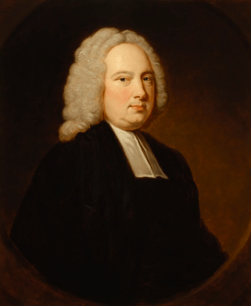
Fig. 4 James Bradley.
James Bradley was a rising star in the scientific circles of England. He came from a modest background but had the good fortune that his mother’s brother, James Pound, was a noted amateur astronomer who had set up a small observatory at his rectory in Wanstead. Bradley showed an early interest in astronomy, and Pound encouraged him, helping with the finances of his education that took him to degrees at Baliol College at Oxford. Even more fortunate was the fact that Pound’s close friend was the Astronomer Royal Edmund Halley, who also took a special interest in Bradley. With Halley’s encouragement, Bradley made important measurements of Mars and several nebulae, demonstrating an ability to work with great accuracy. Halley was impressed and nominated Bradley to the Royal Society in 1718, telling everyone that Bradley was destined to be one of the great astronomers of his time.
Molyneux must have sensed immediately that he had chosen wisely by selecting Bradley to help him with the parallax measurements. Bradley was capable of exceedingly precise work and was fluent mathematically with the geometric complexities of celestial orbits. Fastening the large zenith sector to the chimney of the house gave the apparatus great stability, and in December of 1725 they commenced observations of Gamma Draconis as it passed directly overhead. Because of the accuracy of the sector, they quickly observed a deviation in the star’s position, but the deviation was in the wrong direction, just as Picard had observed. They continued to make observations over two years, obtaining a detailed map of a yearly wobble in the star’s position as it changed angle by 40 seconds of arc (about one percent of a degree) over six months.
When Molyneux was appointed Lord of the Admiralty in 1727, as well as becoming a member of the Irish Parliament (representing Dublin University), he had little time to continue with the observations of Gamma Draconis. He helped Bradley set up a Zenith sector telescope at Bradley’s uncle’s observatory in Wanstead that had a wider field of view to observe more stars, and then he left the project to his friend. A few months later, before either he or Bradley had understood the cause of the stellar aberration, Molyneux collapsed while in the House of Commons and was carried back to his house. One of Molyneux’s many friends was the court anatomist Nathaniel St. André who attended to him over the next several days as he declined and died. St. André was already notorious for roles he had played in several public hoaxes, and on the night of his friend’s death, before the body had grown cold, he eloped with Molyneux’s wife, raising accusations of murder (that could never be proven).
James Bradley and the Light Wind
Over the following year, Bradley observed aberrations in several stars, all of them displaying the same yearly wobble of about 40 seconds of arc. This common behavior of numerous stars demanded a common explanation, something they all shared. It is said that the answer came to Bradley while he was boating on the Thames. The story may be apocryphal, but he apparently noticed the banner fluttering downwind at the top of the mast, and after the boat came about, the banner pointed in a new direction. The wind direction itself had not altered, but the motion of the boat relative to the wind had changed. Light at that time was considered to be made of a flux of corpuscles, like a gentle wind of particles. As the Earth orbited the Sun, its motion relative to this wind would change periodically with the seasons, and the apparent direction of the star would shift a little as a result.
Fig. 5 Principle of stellar aberration. On the left is the rest frame of the star positioned directly overhead as a moving telescope tube must be slightly tilted at an angle (equal to the arctangent of the ratio of the Earth’s speed to the speed of light–greatly exaggerated in the figure) to allow the light to pass through it. On the right is the rest frame of the telescope in which the angular position of the star appears shifted.
Bradley shared his observations and his explanation in a letter to Halley that was read before the Royal Society in January of 1729. Based on his observations, he calculated the speed of light to be about ten thousand times faster than the speed of the Earth in its orbit around the Sun. At that speed, it should take light eight minutes and twelve seconds to travel from the Sun to the Earth (the actual number is eight minutes and 19 seconds). This number was accurate to within a percent of the true value compared with the estimates made by Huygens from the eclipses of the moons of Jupiter that were in error by 27 percent. In addition, because he was unable to discern any effect of parallax in the stellar motions, Bradley was able to place a limit on how far the distant stars must be, more than 100,000 times farther the distance of the Earth from the Sun, which was much farther away than any had previously expected. In January of 1729 the size of the universe suddenly jumped to an incomprehensibly large scale.
Bradley’s explanation of the aberration of starlight was simple and matched observations with good quantitative accuracy. The particle nature of light made it like a wind, or a current, and the motion of the Earth was just a case of Galilean relativity that any freshman physics student can calculate. At first there seemed to be no controversy or difficulties with this interpretation. However, an obscure paper published in 1784 by an obscure English natural philosopher named John Michell (the first person to conceive of a “dark star”) opened a Pandora’s box that launched the crisis of the luminiferous ether and the eventual triumph of Einstein’s theory of Relativity (see Chapter 3 of Interference (Oxford, 2023)), .
By David D. Nolte, Sept. 27, 2023
Read more in Books by David Nolte at Oxford University Press
The constellation Orion strides high across the heavens on cold crisp winter nights in the North, followed at his heel by his constant companion, Canis Major, the Great Dog. Blazing blue from the Dog’s proud chest is the star Sirius, the Dog Star, the brightest star in the night sky. Although it is only the seventh closest star system to our sun, the other six systems host dimmer dwarf stars. Sirius, on the other hand, is a young bright star burning blue in the night. It is an infant star, really, only as old as 5% the age of our sun, coming into being when Dinosaurs walked our planet.
The Sirius star system is a microcosm of mankind’s struggle to understand the Universe. Because it is close and bright, it has become the de facto bench-test for new theories of astrophysics as well as for new astronomical imaging technologies. It has played this role from the earliest days of history, when it was an element of religion rather than of science, down to the modern age as it continues to test and challenge new ideas about quantum matter and extreme physics.
Sirius Through the Ages
To the ancient Egyptians, Sirius was the star Sopdet, the welcome herald of the flooding of the Nile when it rose in the early morning sky of autumn. The star was associated with Isis of the cow constellation Hathor (Canis Major) following closely behind Osiris (Orion). The importance of the annual floods for the well-being of the ancient culture cannot be underestimated, and entire religions full of symbolic significance revolved around the heliacal rising of Sirius.
Fig. Canis Major.
To the Greeks, Sirius was always Sirius, although no one even as far back as Hesiod in the 7th century BC could recall where it got its name. It was the dog star, as it was also to the Persians and the Hindus who called it Tishtrya and Tishya, respectively. The loss of the initial “T” of these related Indo-European languages is a historical sound shift in relation to “S”, indicating that the name of the star dates back at least as far as the divergence of the Indo-European languages around the fourth millennium BC. (Even more intriguing is the same association of Sirius with dogs and wolves by the ancient Chinese and by Alaskan Innuits, as well as by many American Indian tribes, suggesting that the cultural significance of the star, if not its name, may have propagated across Asia and the Bering Strait as far back as the end of the last Ice Age.) As the brightest star of the sky, this speaks to an enduring significance for Sirius, dating back to the beginning of human awareness of our place in nature. No culture was unaware of this astronomical companion to the Sun and Moon and Planets.
The Greeks, too, saw Sirius as a harbinger, not for life-giving floods, but rather of the sweltering heat of late summer. Homer, in the Iliad, famously wrote:
And aging Priam was the first to see him

sparkling on the plain, bright as that star

in autumn rising, whose unclouded rays

shine out amid a throng of stars at dusk—

the one they call Orion's dog, most brilliant,

yes, but baleful as a sign: it brings

great fever to frail men. So pure and bright

the bronze gear blazed upon him as he ran.
The Romans expanded on this view, describing “the dog days of summer”, which is a phrase that echoes till today as we wait for the coming coolness of autumn days.
The Heavens Move
The irony of the Copernican system of the universe, when it was proposed in 1543 by Nicolaus Copernicus, is that it took stars that moved persistently through the heavens and fixed them in the sky, unmovable. The “fixed stars” became the accepted norm for several centuries, until the peripatetic Edmund Halley (1656 – 1742) wondered if the stars really did not move. From Newton’s new work on celestial dynamics (the famous Principia, which Halley generously paid out of his own pocket to have published not only because of his friendship with Newton, but because Halley believed it to be a monumental work that needed to be widely known), it was understood that gravitational effects would act on the stars and should cause them to move.
Fig. Halley’s Comet
In 1710 Halley began studying the accurate star-location records of Ptolemy from one and a half millennia earlier and compared them with what he could see in the night sky. He realized that the star Sirius had shifted in the sky by an angular distance equivalent to the diameter of the moon. Other bright stars, like Arcturus and Procyon, also showed discrepancies from Ptolemy. On the other hand, dimmer stars, that Halley reasoned were farther away, showed no discernible shifts in 1500 years. At a time when stellar parallax, the apparent shift in star locations caused by the movement of the Earth, had not yet been detected, Halley had found an alternative way to get at least some ranked distances to the stars based on their proper motion through the universe. Closer stars to the Earth would show larger angular displacements over 1500 years than stars farther away. By being the closest bright star to Earth, Sirius had become a testbed for observations and theories of the motions of stars. With the confidence of the confirmation of the nearness of Sirius to the Earth, Jacques Cassini claimed in 1714 to have measured the parallax of Sirius, but Halley refuted this claim in 1720. Parallax would remain elusive for another hundred years to come.
The Sound of Sirius
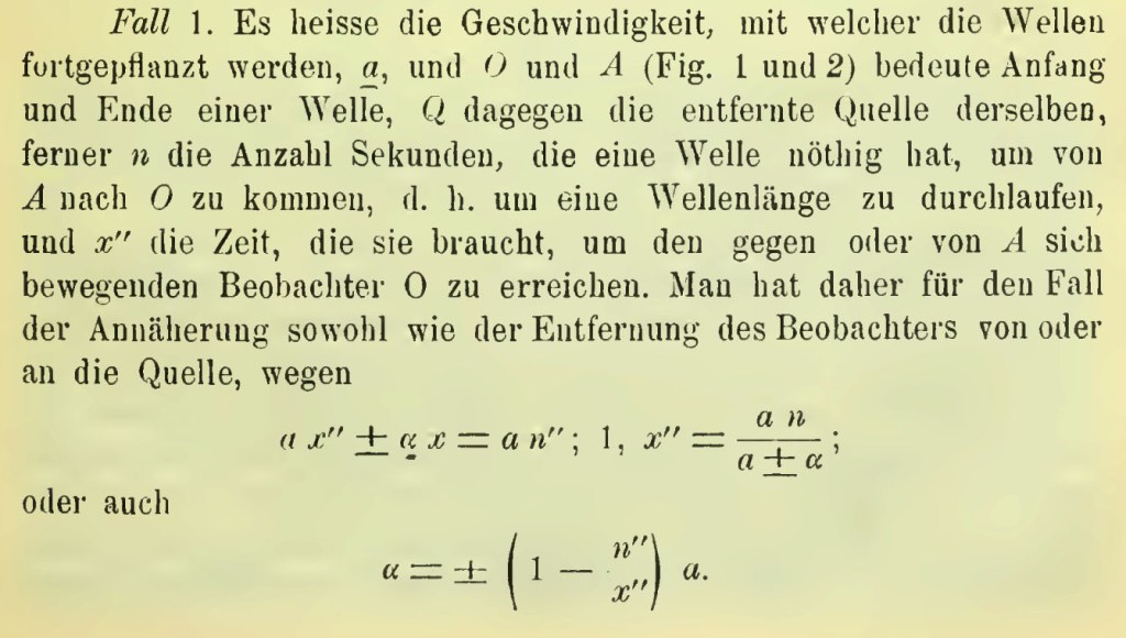
Of all the discoveries that emerged from nineteenth century physics—Young’s fringes, Biot-Savart law, Fresnel lens, Carnot cycle, Faraday effect, Maxwell’s equations, Michelson interferometer—only one is heard daily—the Doppler effect [1]. Christian Doppler’s name is invoked every time you turn on the evening news to watch Doppler weather radar. Doppler’s effect is experienced as you wait by the side of the road for a car to pass by or a jet to fly overhead. Einstein may have the most famous name in physics, but Doppler’s is certainly the most commonly used.
Although experimental support for the acoustic Doppler effect accumulated quickly, corresponding demonstrations of the optical Doppler effect were slow to emerge. The breakthrough in the optical Doppler effect was made by William Huggins (1824-1910). Huggins was an early pioneer in astronomical spectroscopy and was famous for having discovered that some bright nebulae consist of atomic gases (planetary nebula in our own galaxy) while others (later recognized as distant galaxies) consist of unresolved emitting stars. Huggins was intrigued by the possibility of using the optical Doppler effect to measure the speed of stars, and he corresponded with James Clerk Maxwell (1831-1879) to confirm the soundness of Doppler’s arguments, which Maxwell corroborated using his new electromagnetic theory. With the resulting confidence, Huggins turned his attention to the brightest star in the heavens, Sirius, and on May 14, 1868, he read a paper to the Royal Society of London claiming an observation of Doppler shifts in the spectral lines of the star Sirius consistent with a speed of about 50 km/sec [2].
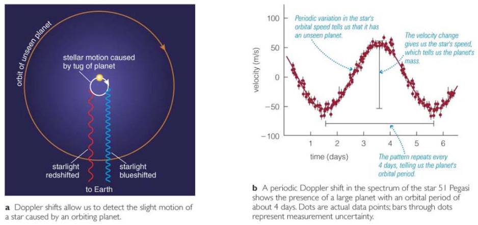
Fig. Doppler spectroscopy of stellar absorption lines caused by the relative motion of the star (in this illustration the orbiting exoplanet is causing the star to wobble.)
The importance of Huggins’ report on the Doppler effect from Sirius was more psychological than scientifically accurate, because it convinced the scientific community that the optical Doppler effect existed. Around this time the German astronomer Hermann Carl Vogel (1841 – 1907) of the Potsdam Observatory began working with a new spectrograph designed by Johann Zöllner from Leipzig [3] to improve the measurements of the radial velocity of stars (the speed along the line of sight). He was aware that the many values quoted by Huggins and others for stellar velocities were nearly the same as the uncertainties in their measurements. Vogel installed photographic capabilities in the telescope and spectrograph at the Potsdam Observatory [4] in 1887 and began making observations of Doppler line shifts in stars through 1890. He published an initial progress report in 1891, and then a definitive paper in 1892 that provided the first accurate stellar radial velocities [5]. Fifty years after Doppler read his paper to the Royal Bohemian Society of Science (in 1842 to a paltry crowd of only a few scientists), the Doppler effect had become an established workhorse of quantitative astrophysics. A laboratory demonstration of the optical Doppler effect was finally achieved in 1901 by Aristarkh Belopolsky (1854-1934), a Russian astronomer, by constructing a device with a narrow-linewidth light source and rapidly rotating mirrors [6].
White Dwarf
While measuring the position of Sirius to unprecedented precision, the German astronomer Friedrich Wilhelm Bessel (1784 – 1846) noticed a slow shift in its position. (This is the same Bessel as “Bessel function” fame, although the functions were originally developed by Daniel Bernoulli and Bessel later generalized them.) Bessel deduced that Sirius must have an unseen companion with an orbital of around 50 years. This companion was discovered by accident in 1862 during a test run of a new lens manufactured by the Clark&Sons glass manufacturing company prior to delivery to Northwestern University in Chicago. (The lens was originally ordered by the University of Mississippi in 1860, but after the Civil War broke out, the Massachusetts-based Clark company put it up for bid. Harvard wanted it, but Northwestern got it.) Sirius itself was redesignated Sirius A, while this new star was designated Sirius B (and sometimes called “The Pup”).
Fig. White dwarf and planet.
The Pup’s spectrum was measured in 1915 by Walter Adams (1876 – 1956) which put it in the newly-formed class of “white dwarf” stars that were very small but, unlike other types of dwarf stars, they had very hot (white) spectra. The deflection of the orbit of Sirius A allowed its mass to be estimated at about one solar mass, which was normal for a dwarf star. Furthermore, its brightness and surface temperature allowed its density to be estimated, but here an incredible number came out: the density of Sirius B was about 30,000 times greater than the density of the sun! Astronomers at the time thought that this was impossible, and Arthur Eddington, who was the expert in star formation, called it “nonsense”. This nonsense withstood all attempts to explain it for over a decade.
In 1926, R. H. Fowler (1889 – 1944) at Cambridge University in England applied the newly-developed theory of quantum mechanics and the Pauli exclusion principle to the problem of such ultra-dense matter. He found that the Fermi sea of electrons provided a type of pressure, called degeneracy pressure, that counteracted the gravitational pressure that threatened to collapse the star under its own weight. Several years later, Subrahmanyan Chandrasekhar calculated the upper limit for white dwarfs using relativistic effects and accurate density profiles and found that a white dwarf with a mass greater than about 1.5 times the mass of the sun would no longer be supported by the electron degeneracy pressure and would suffer gravitational collapse. At the time, the question of what it would collapse to was unknown, although it was later understood that it would collapse to a neutron star. Sirius B, at about one solar mass, is well within the stable range of white dwarfs.
But this was not the end of the story for Sirius B [7]. At around the time that Adams was measuring the spectrum of the white dwarf, Einstein was predicting that light emerging from a dense star would have its wavelengths gravitationally redshifted relative to its usual wavelength. This was one of the three classic tests he proposed for his new theory of General Relativity. (1 – The precession of the perihelion of Mercury. 2 – The deflection of light by gravity. 3 – The gravitational redshift of photons rising out of a gravity well.) Adams announced in 1925 (after the deflection of light by gravity had been confirmed by Eddington in 1919) that he had measured the gravitational redshift. Unfortunately, it was later surmised that he had not measured the gravitational effect but had actually measured Doppler-shifted spectra because of the rotational motion of the star. The true gravitational redshift of Sirius B was finally measured in 1971, although the redshift of another white dwarf, 40 Eridani B, had already been measured in 1954.
Static Interference
The quantum nature of light is an elusive quality that requires second-order experiments of intensity fluctuations to elucidate them, rather than using average values of intensity. But even in second-order experiments, the manifestations of quantum phenomenon are still subtle, as evidenced by an intense controversy that was launched by optical experiments performed in the 1950’s by a radio astronomer, Robert Hanbury Brown (1916 – 2002). (For the full story, see Chapter 4 in my book Interference from Oxford (2023) [8]).
Hanbury Brown (he never went by his first name) was born in Aruvankandu, India, the son of a British army officer. He never seemed destined for great things, receiving an unremarkable education that led to a degree in radio engineering from a technical college in 1935. He hoped to get a PhD in radio technology, and he even received a scholarship to study at Imperial College in London, when he was urged by the rector of the university, Sir Henry Tizard, to give up his plans and join an effort to develop defensive radar against a growing threat from Nazi Germany as it aggressively rearmed after abandoning the punitive Versailles Treaty. Hanbury Brown began the most exciting and unnerving five years of his life, right in the middle of the early development of radar defense, leading up to the crucial role it played in the Battle of Britain in 1940 and the Blitz from 1940 to 1941. Partly due to the success of radar, Hitler halted night-time raids in the Spring of 1941, and England escaped invasion.
In 1949, fourteen years after he had originally planned to start his PhD, Hanbury Brown enrolled at the relatively ripe age of 33 at the University of Manchester. Because of his background in radar, his faculty advisor told him to look into the new field of radio astronomy that was just getting started, and Manchester was a major player because it administrated the Jodrell Bank Observatory, which was one of the first and largest radio astronomy observatories in the World. Hanbury Brown was soon applying all he had learned about radar transmitters and receivers to the new field, focusing particularly on aspects of radio interferometry after Martin Ryle (1918 – 1984) at Cambridge with Derek Vonberg (1921 – 2015) developed the first radio interferometer to measure the angular size of the sun [9] and of radio sources on the Sun’s surface that were related to sunspots [10]. Despite the success of their measurements, their small interferometer was unable to measure the size of other astronomical sources. From Michelson’s formula for stellar interferometry, longer baselines between two separated receivers would be required to measure smaller angular sizes. For his PhD project, Hanbury Brown was given the task of designing a radio interferometer to resolve the two strongest radio sources in the sky, Cygnus A and Cassiopeia A, whose angular sizes were unknown. As he started the project, he was confronted with the problem of distributing a stable reference signal to receivers that might be very far apart, maybe even thousands of kilometers, a problem that had no easy solution.
After grappling with this technical problem for months without success, late one night in 1949 Hanbury Brown had an epiphany [11], wondering what would happen if the two separate radio antennas measured only intensities rather than fields. The intensity in a radio telescope fluctuates in time like random noise. If that random noise were measured at two separated receivers while trained on a common source, would those noise patterns look the same? After a few days considering this question, he convinced himself that the noise would indeed share common features, and the degree to which the two noise traces were similar should depend on the size of the source and the distance between the two receivers, just like Michelson’s fringe visibility. But his arguments were back-of-the-envelope, so he set out to find someone with the mathematical skills to do it more rigorously. He found Richard Twiss.
Richard Quentin Twiss (1920 – 2005), like Hanbury Brown, was born in India to British parents but had followed a more prestigious educational path, taking the Mathematical Tripos exam at Cambridge in 1941 and receiving his PhD from MIT in the United States in 1949. He had just returned to England, joining the research division of the armed services located north of London, when he received a call from Hanbury Brown at the Jodrell Bank radio astronomy laboratory in Manchester. Twiss travelled to meet Hanbury Brown in Manchester, who put him up in his flat in the neighboring town of Wilmslow. The two set up the mathematical assumptions behind the new “intensity interferometer” and worked late into the night. When Hanbury Brown finally went to bed, Twiss was still figuring the numbers. The next morning, the tall and lanky Twiss appeared in his silk dressing gown in the kitchen and told Hanbury Brown, “This idea of yours is no good, it doesn’t work”[12]—it would never be strong enough to detect the intensity from stars. However, after haggling over the details of some of the integrals, Hanbury Brown, and then finally Twiss, became convinced that the effect was real. Rather than fringe visibility, it was the correlation coefficient between two noise signals that would depend on the joint sizes of the source and receiver in a way that captured the same information as Michelson’s first-order fringe visibility. But because no coherent reference wave was needed for interferometric mixing, this new approach could be carried out across very large baseline distances.
After demonstrating the effect on astronomical radio sources, Hanbury Brown and Twiss took the next obvious step: optical stellar intensity interferometry. Their work had shown that photon noise correlations were analogous to Michelson fringe visibility, so the stellar intensity interferometer was expected to work similarly to the Michelson stellar interferometer—but with better stability over much longer baselines because it did not need a reference. An additional advantage was the simple light collecting requirements. Rather than needing a pair of massively expensive telescopes for high-resolution imaging, the intensity interferometer only needed to point two simple light collectors in a common direction. For this purpose, and to save money, Hanbury Brown selected two of the largest army-surplus anti-aircraft searchlights that he could find left over from the London Blitz. The lamps were removed and replaced with high-performance photomultipliers, and the units were installed on two train cars that could run along a railroad siding that crossed the Jodrell Bank grounds.
Fig. Stellar Interferometers: (Left) Michelson Stellar Field Interferometer. (Right) Hanbury Brown Twiss Stellar Intensity Interferometer.
The target of the first test of the intensity interferometer was Sirius, the Dog Star. Sirius was chosen because it is the brightest star in the night sky and was close to Earth at 8.6 light years and hence would be expected to have a relatively large angular size. The observations began at the start of winter in 1955, but the legendary English weather proved an obstacle. In addition to endless weeks of cloud cover, on many nights dew formed on the reflecting mirrors, making it necessary to install heaters. It took more than three months to make 60 operational attempts to accumulate a mere 18 hours of observations [13]. But it worked! The angular size of Sirius was measured for the first time. It subtended an angle of approximately 6 milliarcseconds (mas), which was well within the expected range for such a main sequence blue star. This angle is equivalent to observing a house on the Moon from the Earth. No single non-interferometric telescope on Earth, or in Earth orbit, has that kind of resolution, even today. Once again, Sirus was the testbed of a new observational technology. Hanbury Brown and Twiss went on the measure the diameters of dozens of stars.
Adaptive Optics
Any undergraduate optics student can tell you that bigger telescopes have higher spatial resolution. But this is only true up to a point. When telescope diameters become not much bigger than about 10 inches, the images they form start to dance, caused by thermal fluctuations in the atmosphere. Large telescopes can still get “lucky” at moments when the atmosphere is quiet, but this usually only happens for a fraction of a second before the fluctuation set in again. This is the primary reason that the Hubble Space Telescope was placed in Earth orbit above the atmosphere, and why the James Webb Space Telescope is flying a million miles away from the Earth. But that is not the end of Earth-based large telescoped. The Very Large Telescope (VLT) has a primary diameter of 8 meters, and the Extremely Large Telescope (ELT), coming online soon, has an even bigger diameter of 40 meters. How do these work under the atmospheric blanket? The answer is adaptive optics.
Adaptive optics uses active feedback to measure the dancing images caused by the atmosphere and uses the information to control a flexible array of mirror elements to exactly cancel out the effects of the atmospheric fluctuations. In the early days of adaptive-optics development, the applications were more military than astronomic, but advances made in imaging enemy satellites soon was released to the astronomers. The first civilian demonstrations of adaptive optics were performed in 1977 when researchers at Bell Labs [14] and at the Space Sciences Lab at UC Berkeley [15] each made astronomical demonstrations of improved seeing of the star Sirius using adaptive optics. The field developed rapidly after that, but once again Sirius had led the way.
Star Travel
The day is fast approaching when humans will begin thinking seriously of visiting nearby stars—not in person at first, but with unmanned spacecraft that can telemeter information back to Earth. Although Sirius is not the closest star to Earth—it is 8.6 lightyears away while Alpha Centauri is almost twice as close at only 4.2 lightyears away—it may be the best target for an unmanned spacecraft. The reason is its brightness.
Stardrive technology is still in its infancy—most of it is still on drawing boards. Therefore, the only “mature” technology we have today is light pressure on solar sails. Within the next 50 years or so we will have the technical ability to launch a solar sail towards a nearby star and accelerate it to a good fraction of the speed of light. The problem is decelerating the spaceship when it arrives at its destination, otherwise it will go zipping by with only a few seconds to make measurements after its long trek there.
Fig. NASA’s solar sail demonstrator unit (artist’s rendering).
A better idea is to let the star light push against the solar sail to decelerate it to orbital speed by the time it arrives. That way, the spaceship can orbit the target star for years. This is a possibility with Sirius. Because it is so bright, its light can decelerate the spaceship even when it is originally moving at relativistic speeds. By one calculation, the trip to Sirius, including the deceleration and orbital insertion, should only take about 69 years [16]. That’s just one lifetime. Signals could be beaming back from Sirius by as early as 2100—within the lifetimes of today’s children.
[2] W. Huggins, “Further observations on the spectra of some of the stars and nebulae, with an attempt to determine therefrom whether these bodies are moving towards or from the earth, also observations on the spectra of the sun and of comet II,” Philos. Trans. R. Soc. London vol. 158, pp. 529-564, 1868. The correct value is -5.5 km/sec approaching Earth. Huggins got the magnitude and even the sign wrong.
[3] in Hearnshaw, The Analysis of Starlight (Cambridge University Press, 2014), pg. 89
[4] The Potsdam Observatory was where the American Albert Michelson built his first interferometer while studying with Helmholtz in Berlin.
[5] Vogel, H. C. Publik. der astrophysik. Observ. Potsdam1: 1. (1892)
[6] A. Belopolsky, “On an apparatus for the laboratory demonstration of the Doppler-Fizeau principle,” Astrophysical Journal, vol. 13, pp. 15-24, Jan 1901.
[9] M. Ryle and D. D. Vonberg, “Solar Radiation on 175 Mc/sec,” Nature, vol. 158 (1946): pp. 339-340.; K. I. Kellermann and J. M. Moran, “The development of high-resolution imaging in radio astronomy,” Annual Review of Astronomy and Astrophysics, vol. 39, (2001): pp. 457-509.
[10] M. Ryle, ” Solar radio emissions and sunspots,” Nature, vol. 161, no. 4082 (1948): pp. 136-136.
[11] R. H. Brown, The intensity interferometer; its application to astronomy (London, New York, Taylor & Francis; Halsted Press, 1974).
[12] R. H. Brown, Boffin : A personal story of the early days of radar and radio astronomy (Adam Hilger, 1991), p. 106.
[13] R. H. Brown and R. Q. Twiss. ” Test of a new type of stellar interferometer on Sirius.” Nature178, no. 4541 (1956): pp. 1046-1048.
[14] S. L. McCall, T. R. Brown, and A. Passner, “IMPROVED OPTICAL STELLAR IMAGE USING A REAL-TIME PHASE-CORRECTION SYSTEM – INITIAL RESULTS,” Astrophysical Journal, vol. 211, no. 2, pp. 463-468, (1977)
[15] A. Buffington, F. S. Crawford, R. A. Muller, and C. D. Orth, “1ST OBSERVATORY RESULTS WITH AN IMAGE-SHARPENING TELESCOPE,” Journal of the Optical Society of America, vol. 67, no. 3, pp. 304-305, 1977 (1977)
This history of interferometry has many surprising back stories surrounding the scientists who discovered and explored one of the most important aspects of the physics of light—interference. From Thomas Young who first proposed the law of interference, and Augustin Fresnel and Francois Arago who explored its properties, to Albert Michelson, who went almost mad grappling with literal firestorms surrounding his work, these scientists overcame personal and professional obstacles on their quest to uncover light’s secrets. The book’s stories, told around the topic of optics, tells us something more general about human endeavor as scientists pursue science.
Interference: The History of Optical Interferometry and the Scientists who Tamed Light, was published Ag. 6 and is available at Oxford University Press and Amazon. Here is a brief preview of the frist several chapters:
Chapter 1. Thomas Young Polymath: The Law of Interference
Thomas Young was the ultimate dabbler, his interests and explorations ranged far and wide, from ancient egyptology to naval engineering, from physiology of perception to the physics of sound and light. Yet unlike most dabblers who accomplish little, he made original and seminal contributions to all these fields. Some have called him the “Last Man Who Knew Everything”.
Thomas Young. The Law of Interference.
The chapter, Thomas Young Polymath: The Law of Interference, begins with the story of the invasion of Egypt in 1798 by Napoleon Bonaparte as the unlikely link among a set of epic discoveries that launched the modern science of light. The story of interferometry passes from the Egyptian campaign and the discovery of the Rosetta Stone to Thomas Young. Young was a polymath, known for his facility with languages that helped him decipher Egyptian hieroglyphics aided by the Rosetta Stone. He was also a city doctor who advised the admiralty on the construction of ships, and he became England’s premier physicist at the beginning of the nineteenth century, building on the wave theory of Huygens, as he challenged Newton’s particles of light. But his theory of the wave nature of light was controversial, attracting sharp criticism that would pass on the task of refuting Newton to a new generation of French optical physicists.
Chapter 2. The Fresnel Connection: Particles versus Waves
Augustin Fresnel was an intuitive genius whose talents were almost squandered on his job building roads and bridges in the backwaters of France until he was discovered and rescued by Francois Arago.
The Fresnel Connection: Particles versus Waves describes the campaign of Arago and Fresnel to prove the wave nature of light based on Fresnel’s theory of interfering waves in diffraction. Although the discovery of the polarization of light by Etienne Malus posed a stark challenge to the undulationists, the application of wave interference, with the superposition principle of Daniel Bernoulli, provided the theoretical framework for the ultimate success of the wave theory. The final proof came through the dramatic demonstration of the Spot of Arago.
Chapter 3. At Light Speed: The Birth of Interferometry
There is no question that Francois Arago was a swashbuckler. His life’s story reads like an adventure novel as he went from being marooned in hostile lands early in his career to becoming prime minister of France after the 1848 revolutions swept across Europe.
At Light Speed: The Birth of Interferometry tells how Arago attempted to use Snell’s Law to measure the effect of the Earth’s motion through space but found no effect, in contradiction to predictions using Newton’s particle theory of light. Direct measurements of the speed of light were made by Hippolyte Fizeau and Leon Foucault who originally began as collaborators but had an epic falling-out that turned into an intense competition. Fizeau won priority for the first measurement, but Foucault surpassed him by using the Arago interferometer to measure the speed of light in air and water with increasing accuracy. Jules Jamin later invented one of the first interferometric instruments for use as a refractometer.
Chapter 4. After the Gold Rush: The Trials of Albert Michelson
No name is more closely connected to interferometry than that of Albert Michelson. He succeeded, sometimes at great personal cost, in launching interferometric metrology as one of the most important tools used by scientists today.
Albert A. Michelson, 1907 Nobel Prize. Image Credit.
After the Gold Rush: The Trials of Albert Michelson tells the story of Michelson’s youth growing up in the gold fields of California before he was granted an extraordinary appointment to Annapolis by President Grant. Michelson invented his interferometer while visiting Hermann von Helmholtz in Berlin, Germany, as he sought to detect the motion of the Earth through the luminiferous ether, but no motion was detected. After returning to the States and a faculty position at Case University, he met Edward Morley, and the two continued the search for the Earth’s motion, concluding definitively its absence. The Michelson interferometer launched a menagerie of interferometers (including the Fabry-Perot interferometer) that ushered in the golden age of interferometry.
Chapter 5. Stellar Interference: Measuring the Stars
Learning from his attempts to measure the speed of light through the ether, Michelson realized that the partial coherence of light from astronomical sources could be used to measure their sizes. His first measurements using the Michelson Stellar Interferometer launched a major subfield of astronomy that is one of the most active today.
R Hanbury Brown
Stellar Interference: Measuring the Stars brings the story of interferometry to the stars as Michelson proposed stellar interferometry, first demonstrated on the Galilean moons of Jupiter, followed by an application developed by Karl Schwarzschild for binary stars, and completed by Michelson with observations encouraged by George Hale on the star Betelgeuse. However, the Michelson stellar interferometry had stability limitations that were overcome by Hanbury Brown and Richard Twiss who developed intensity interferometry based on the effect of photon bunching. The ultimate resolution of telescopes was achieved after the development of adaptive optics that used interferometry to compensate for atmospheric turbulence.
And More
The last 5 chapters bring the story from Michelson’s first stellar interferometer into the present as interferometry is used today to search for exoplanets, to image distant black holes half-way across the universe and to detect gravitational waves using the most sensitive scientific measurement apparatus ever devised.
Chapter 6. Across the Universe: Exoplanets, Black Holes and Gravitational Waves
Moving beyond the measurement of star sizes, interferometry lies at the heart of some of the most dramatic recent advances in astronomy, including the detection of gravitational waves by LIGO, the imaging of distant black holes and the detection of nearby exoplanets that may one day be visited by unmanned probes sent from Earth.
Chapter 7. Two Faces of Microscopy: Diffraction and Interference
The complement of the telescope is the microscope. Interference microscopy allows invisible things to become visible and for fundamental limits on image resolution to be blown past with super-resolution at the nanoscale, revealing the intricate workings of biological systems with unprecedented detail.
Chapter 8. Holographic Dreams of Princess Leia: Crossing Beams
Holography is the direct legacy of Young’s double slit experiment, as coherent sources of light interfere to record, and then reconstruct, the direct scattered fields from illuminated objects. Holographic display technology promises to revolutionize virtual reality.
Chapter 9. Photon Interference: The Foundations of Quantum Communication and Computing
Quantum information science, at the forefront of physics and technology today, owes much of its power to the principle of interference among single photons.
Chapter 10. The Quantum Advantage: Interferometric Computing
Photonic quantum systems have the potential to usher in a new information age using interference in photonic integrated circuits.
A popular account of the trials and toils of the scientists and engineers who tamed light and used it to probe the universe.
Hyperspace by any other name would sound as sweet, conjuring to the mind’s eye images of hypercubes and tesseracts, manifolds and wormholes, Klein bottles and Calabi Yau quintics. Forget the dimension of time—that may be the most mysterious of all—but consider the extra spatial dimensions that challenge the mind and open the door to dreams of going beyond the bounds of today’s physics.
The geometry of n dimensions studies reality; no one doubts that. Bodies in hyperspace are subject to precise definition, just like bodies in ordinary space; and while we cannot draw pictures of them, we can imagine and study them.
(Poincare 1895)
Here is a short history of hyperspace. It begins with advances by Möbius and Liouville and Jacobi who never truly realized what they had invented, until Cayley and Grassmann and Riemann made it explicit. They opened Pandora’s box, and multiple dimensions burst upon the world never to be put back again, giving us today the manifolds of string theory and infinite-dimensional Hilbert spaces.
August Möbius (1827)
Although he is most famous for the single-surface strip that bears his name, one of the early contributions of August Möbius was the idea of barycentric coordinates [1] , for instance using three coordinates to express the locations of points in a two-dimensional simplex—the triangle. Barycentric coordinates are used routinely today in metallurgy to describe the alloy composition in ternary alloys.
Möbius’ work was one of the first to hint that tuples of numbers could stand in for higher dimensional space, and they were an early example of homogeneous coordinates that could be used for higher-dimensional representations. However, he was too early to use any language of multidimensional geometry.
Carl Jacobi (1834)
Carl Jacobi was a master at manipulating multiple variables, leading to his development of the theory of matrices. In this context, he came to study (n-1)-fold integrals over multiple continuous-valued variables. From our modern viewpoint, he was evaluating surface integrals of hyperspheres.
Carl Gustav Jacob Jacobi (1804 – 1851)
In 1834, Jacobi found explicit solutions to these integrals and published them in a paper with the imposing title “De binis quibuslibet functionibus homogeneis secundi ordinis per substitutiones lineares in alias binas transformandis, quae solis quadratis variabilium constant; una cum variis theorematis de transformatione et determinatione integralium multiplicium” [2]. The resulting (n-1)-fold integrals are
when the space dimension is even or odd, respectively. These are the surface areas of the manifolds called (n-1)-spheres in n-dimensional space. For instance, the 2-sphere is the ordinary surface 4πr2 of a sphere on our 3D space.
Despite the fact that we recognize these as surface areas of hyperspheres, Jacobi used no geometric language in his paper. He was still too early, and mathematicians had not yet woken up to the analogy of extending spatial dimensions beyond 3D.
Joseph Liouville (1838)
Joseph Liouville’s name is attached to a theorem that lies at the core of mechanical systems—Liouville’s Theorem that proves that volumes in high-dimensional phase space are incompressible. Surprisingly, Liouville had no conception of high dimensional space, to say nothing of abstract phase space. The story of the convoluted path that led Liouville’s name to be attached to his theorem is told in Chapter 6, “The Tangled Tale of Phase Space”, in Galileo Unbound (Oxford University Press, 2018).
Joseph Liouville (1809 – 1882)
Nonetheless, Liouville did publish a pure-mathematics paper in 1838 in Crelle’s Journal [3] that identified an invariant quantity that stayed constant during the differential change of multiple variables when certain criteria were satisfied. It was only later that Jacobi, as he was developing a new mechanical theory based on William R. Hamilton’s work, realized that the criteria needed for Liouville’s invariant quantity to hold were satisfied by conservative mechanical systems. Even then, neither Liouville nor Jacobi used the language of multidimensional geometry, but that was about to change in a quick succession of papers and books by three mathematicians who, unknown to each other, were all thinking along the same lines.
Facsimile of Liouville’s 1838 paper on invariants
Arthur Cayley (1843)
Arthur Cayley was the first to take the bold step to call the emerging geometry of multiple variables to be actual space. His seminal paper “Chapters in the Analytic Theory of n-Dimensions” was published in 1843 in the Philosophical Magazine [4]. Here, for the first time, Cayley recognized that the domain of multiple variables behaved identically to multidimensional space. He used little of the language of geometry in the paper, which was mostly analysis rather than geometry, but his bold declaration for spaces of n-dimensions opened the door to a changing mindset that would soon sweep through geometric reasoning.
Grassmann’s life story, although not overly tragic, was beset by lifelong setbacks and frustrations. He was a mathematician literally 30 years ahead of his time, but because he was merely a high-school teacher, no-one took his ideas seriously.
Somehow, in nearly a complete vacuum, disconnected from the professional mathematicians of his day, he devised an entirely new type of algebra that allowed geometric objects to have orientation. These could be combined in numerous different ways obeying numerous different laws. The simplest elements were just numbers, but these could be extended to arbitrary complexity with arbitrary number of elements. He called his theory a theory of “Extension”, and he self-published a thick and difficult tome that contained all of his ideas [5]. He tried to enlist Möbius to help disseminate his ideas, but even Möbius could not recognize what Grassmann had achieved.
In fact, what Grassmann did achieve was vector algebra of arbitrarily high dimension. Perhaps more impressive for the time is that he actually recognized what he was dealing with. He did not know of Cayley’s work, but independently of Cayley he used geometric language for the first time describing geometric objects in high dimensional spaces. He said, “since this method of formation is theoretically applicable without restriction, I can define systems of arbitrarily high level by this method… geometry goes no further, but abstract science knows no limits.” [6]
Grassman was convinced that he had discovered something astonishing and new, which he had, but no one understood him. After years trying to get mathematicians to listen, he finally gave up, left mathematics behind, and actually achieved some fame within his lifetime in the field of linguistics. There is even a law of diachronic linguistics named after him. For the story of Grassmann’s struggles, see the blog on Grassmann and his Wedge Product .
Hermann Grassmann (1809 – 1877).
Julius Plücker (1846)
Projective geometry sounds like it ought to be a simple topic, like the projective property of perspective art as parallel lines draw together and touch at the vanishing point on the horizon of a painting. But it is far more complex than that, and it provided a separate gateway into the geometry of high dimensions.
A hint of its power comes from homogeneous coordinates of the plane. These are used to find where a point in three dimensions intersects a plane (like the plane of an artist’s canvas). Although the point on the plane is in two dimensions, it take three homogeneous coordinates to locate it. By extension, if a point is located in three dimensions, then it has four homogeneous coordinates, as if the three dimensional point were a projection onto 3D from a 4D space.
These ideas were pursued by Julius Plücker as he extended projective geometry from the work of earlier mathematicians such as Desargues and Möbius. For instance, the barycentric coordinates of Möbius are a form of homogeneous coordinates. What Plücker discovered is that space does not need to be defined by a dense set of points, but a dense set of lines can be used just as well. The set of lines is represented as a four-dimensional manifold. Plücker reported his findings in a book in 1846 [7] and expanded on the concepts of multidimensional spaces published in 1868 [8].
Julius Plücker (1801 – 1868).
Ludwig Schläfli (1851)
After Plücker, ideas of multidimensional analysis became more common, and Ludwig Schläfli (1814 – 1895), a professor at the University of Berne in Switzerland, was one of the first to fully explore analytic geometry in higher dimensions. He described multidimsnional points that were located on hyperplanes, and he calculated the angles between intersecting hyperplanes [9]. He also investigated high-dimensional polytopes, from which are derived our modern “Schläfli notation“. However, Schläffli used his own terminology for these objects, emphasizing analytic properties without using the ordinary language of high-dimensional geometry.
Some of the polytopes studied by Schläfli.
Bernhard Riemann (1854)
The person most responsible for the shift in the mindset that finally accepted the geometry of high-dimensional spaces was Bernhard Riemann. In 1854 at the university in Göttingen he presented his habilitation talk “Über die Hypothesen, welche der Geometrie zu Grunde liegen” (Over the hypotheses on which geometry is founded). A habilitation in Germany was an examination that qualified an academic to be able to advise their own students (somewhat like attaining tenure in US universities).
The habilitation candidate would suggest three topics, and it was usual for the first or second to be picked. Riemann’s three topics were: trigonometric properties of functions (he was the first to rigorously prove the convergence properties of Fourier series), aspects of electromagnetic theory, and a throw-away topic that he added at the last minute on the foundations of geometry (on which he had not actually done any serious work). Gauss was his faculty advisor and picked the third topic. Riemann had to develop the topic in a very short time period, starting from scratch. The effort exhausted him mentally and emotionally, and he had to withdraw temporarily from the university to regain his strength. After returning around Easter, he worked furiously for seven weeks to develop a first draft and then asked Gauss to set the examination date. Gauss initially thought to postpone to the Fall semester, but then at the last minute scheduled the talk for the next day. (For the story of Riemann and Gauss, see Chapter 4 “Geometry on my Mind” in the book Galileo Unbound (Oxford, 2018)).
Riemann gave his lecture on 10 June 1854, and it was a masterpiece. He stripped away all the old notions of space and dimensions and imbued geometry with a metric structure that was fundamentally attached to coordinate transformations. He also showed how any set of coordinates could describe space of any dimension, and he generalized ideas of space to include virtually any ordered set of measurables, whether it was of temperature or color or sound or anything else. Most importantly, his new system made explicit what those before him had alluded to: Jacobi, Grassmann, Plücker and Schläfli. Ideas of Riemannian geometry began to percolate through the mathematics world, expanding into common use after Richard Dedekind edited and published Riemann’s habilitation lecture in 1868 [10].
In discussions of multidimensional spaces, it is important to step back and ask what is dimension? This question is not as easy to answer as it may seem. In fact, in 1878, George Cantor proved that there is a one-to-one mapping of the plane to the line, making it seem that lines and planes are somehow the same. He was so astonished at his own results that he wrote in a letter to his friend Richard Dedekind “I see it, but I don’t believe it!”. A few decades later, Peano and Hilbert showed how to create area-filling curves so that a single continuous curve can approach any point in the plane arbitrarily closely, again casting shadows of doubt on the robustness of dimension. These questions of dimensionality would not be put to rest until the work by Karl Menger around 1926 when he provided a rigorous definition of topological dimension (see the Blog on the History of Fractals).
Area-filling curves by Peano and Hilbert.
Hermann Minkowski and Spacetime (1908)
Most of the earlier work on multidimensional spaces were mathematical and geometric rather than physical. One of the first examples of physical hyperspace is the spacetime of Hermann Minkowski. Although Einstein and Poincaré had noted how space and time were coupled by the Lorentz equations, they did not take the bold step of recognizing space and time as parts of a single manifold. This step was taken in 1908 [11] by Hermann Minkowski who claimed
“Gentlemen! The views of space and time which I wish to lay before you … They are radical. Henceforth space by itself, and time by itself, are doomed to fade away into mere shadows, and only a kind of union of the two will preserve an independent reality.”Herman Minkowski (1908)
Facsimile of Minkowski’s 1908 publication on spacetime.
Felix Hausdorff and Fractals (1918)
No story of multiple “integer” dimensions can be complete without mentioning the existence of “fractional” dimensions, also known as fractals. The individual who is most responsible for the concepts and mathematics of fractional dimensions was Felix Hausdorff. Before being compelled to commit suicide by being jewish in Nazi Germany, he was a leading light in the intellectual life of Leipzig, Germany. By day he was a brilliant mathematician, by night he was the author Paul Mongré writing poetry and plays.
In 1918, as the war was ending, he wrote a small book “Dimension and Outer Measure” that established ways to construct sets whose measured dimensions were fractions rather than integers [12]. Benoit Mandelbrot would later popularize these sets as “fractals” in the 1980’s. For the background on a history of fractals, see the Blog A Short History of Fractals.
Felix Hausdorff (1868 – 1942)
Example of a fractal set with embedding dimension DE = 2, topological dimension DT = 1, and fractal dimension DH = 1.585.
The Fifth Dimension of Theodore Kaluza (1921) and Oskar Klein (1926)
The first theoretical steps to develop a theory of a physical hyperspace (in contrast to merely a geometric hyperspace) were taken by Theodore Kaluza at the University of Königsberg in Prussia. He added an additional spatial dimension to Minkowski spacetime as an attempt to unify the forces of gravity with the forces of electromagnetism. Kaluza’s paper was communicated to the journal of the Prussian Academy of Science in 1921 through Einstein who saw the unification principles as a parallel of some of his own attempts [13]. However, Kaluza’s theory was fully classical and did not include the new quantum theory that was developing at that time in the hands of Heisenberg, Bohr and Born.
Oskar Klein was a Swedish physicist who was in the “second wave” of quantum physicists having studied under Bohr. Unaware of Kaluza’s work, Klein developed a quantum theory of a five-dimensional spacetime [14]. For the theory to be self-consistent, it was necessary to roll up the extra dimension into a tight cylinder. This is like a strand a spaghetti—looking at it from far away it looks like a one-dimensional string, but an ant crawling on the spaghetti can move in two dimensions—along the long direction, or looping around it in the short direction called a compact dimension. Klein’s theory was an early attempt at what would later be called string theory. For the historical background on Kaluza and Klein, see the Blog on Oskar Klein.
The wave equations of Klein-Gordon, Schrödinger and Dirac.
John Campbell (1931): Hyperspace in Science Fiction
Art has a long history of shadowing the sciences, and the math and science of hyperspace was no exception. One of the first mentions of hyperspace in science fiction was in the story “Islands in Space’, by John Campbell [15], published in the Amazing Stories quarterly in 1931, where it was used as an extraordinary means of space travel.
In 1951, Isaac Asimov made travel through hyperspace the transportation network that connected the galaxy in his Foundation Trilogy [16].
Isaac Asimov (1920 – 1992)
John von Neumann and Hilbert Space (1932)
Quantum mechanics had developed rapidly through the 1920’s, but by the early 1930’s it was in need of an overhaul, having outstripped rigorous mathematical underpinnings. These underpinnings were provided by John von Neumann in his 1932 book on quantum theory [17]. This is the book that cemented the Copenhagen interpretation of quantum mechanics, with projection measurements and wave function collapse, while also establishing the formalism of Hilbert space.
Hilbert space is an infinite dimensional vector space of orthogonal eigenfunctions into which any quantum wave function can be decomposed. The physicists of today work and sleep in Hilbert space as their natural environment, often losing sight of its infinite dimensions that don’t seem to bother anyone. Hilbert space is more than a mere geometrical space, but less than a full physical space (like five-dimensional spacetime). Few realize that what is so often ascribed to Hilbert was actually formalized by von Neumann, among his many other accomplishments like stored-program computers and game theory.
One of the strangest entities inhabiting the theory of spacetime is the Einstein-Rosen Bridge. It is space folded back on itself in a way that punches a short-cut through spacetime. Einstein, working with his collaborator Nathan Rosen at Princeton’s Institute for Advanced Study, published a paper in 1935 that attempted to solve two problems [18]. The first problem was the Schwarzschild singularity at a radius r = 2M/c2 known as the Schwarzschild radius or the Event Horizon. Einstein had a distaste for such singularities in physical theory and viewed them as a problem. The second problem was how to apply the theory of general relativity (GR) to point masses like an electron. Again, the GR solution to an electron blows up at the location of the particle at r = 0.
To eliminate both problems, Einstein and Rosen (ER) began with the Schwarzschild metric in its usual form
where it is easy to see that it “blows up” when r = 2M/c2 as well as at r = 0. ER realized that they could write a new form that bypasses the singularities using the simple coordinate substitution
to yield the “wormhole” metric
It is easy to see that as the new variable u goes from -inf to +inf that this expression never blows up. The reason is simple—it removes the 1/r singularity by replacing it with 1/(r + ε). Such tricks are used routinely today in computational physics to keep computer calculations from getting too large—avoiding the divide-by-zero problem. It is also known as a form of regularization in machine learning applications. But in the hands of Einstein, this simple “bypass” is not just math, it can provide a physical solution.
It is hard to imagine that an article published in the Physical Review, especially one written about a simple variable substitution, would appear on the front page of the New York Times, even appearing “above the fold”, but such was Einstein’s fame this is exactly the response when he and Rosen published their paper. The reason for the interest was because of the interpretation of the new equation—when visualized geometrically, it was like a funnel between two separated Minkowski spaces—in other words, what was named a “wormhole” by John Wheeler in 1957. Even back in 1935, there was some sense that this new property of space might allow untold possibilities, perhaps even a form of travel through such a short cut.
As it turns out, the ER wormhole is not stable—it collapses on itself in an incredibly short time so that not even photons can get through it in time. More recent work on wormholes have shown that it can be stabilized by negative energy density, but ordinary matter cannot have negative energy density. On the other hand, the Casimir effect might have a type of negative energy density, which raises some interesting questions about quantum mechanics and the ER bridge.
Edward Witten’s 10+1 Dimensions (1995)
A history of hyperspace would not be complete without a mention of string theory and Edward Witten’s unification of the variously different 10-dimensional string theories into 10- or 11-dimensional M-theory. At a string theory conference at USC in 1995 he pointed out that the 5 different string theories of the day were all related through dualities. This observation launched the second superstring revolution that continues today. In this theory, 6 extra spatial dimensions are wrapped up into complex manifolds such as the Calabi-Yau manifold.
Two-dimensional slice of a six-dimensional Calabi-Yau quintic manifold.
Prospects
There is definitely something wrong with our three-plus-one dimensions of spacetime. We claim that we have achieved the pinnacle of fundamental physics with what is called the Standard Model and the Higgs boson, but dark energy and dark matter loom as giant white elephants in the room. They are giant, gaping, embarrassing and currently unsolved. By some estimates, the fraction of the energy density of the universe comprised of ordinary matter is only 5%. The other 95% is in some form unknown to physics. How can physicists claim to know anything if 95% of everything is in some unknown form?
The answer, perhaps to be uncovered sometime in this century, may be the role of extra dimensions in physical phenomena—probably not in every-day phenomena, and maybe not even in high-energy particles—but in the grand expanse of the cosmos.
By David D. Nolte, Feb. 8, 2023
Bibliography:
M. Kaku, R. O’Keefe, Hyperspace: A scientific odyssey through parallel universes, time warps, and the tenth dimension. (Oxford University Press, New York, 1994).
A. N. Kolmogorov, A. P. Yushkevich, Mathematics of the 19th century: Geometry, analytic function theory. (Birkhäuser Verlag, Basel ; 1996).
References:
[1] F. Möbius, in Möbius, F. Gesammelte Werke,, D. M. Saendig, Ed. (oHG, Wiesbaden, Germany, 1967), vol. 1, pp. 36-49.
[2] Carl Jacobi, “De binis quibuslibet functionibus homogeneis secundi ordinis per substitutiones lineares in alias binas transformandis, quae solis quadratis variabilium constant; una cum variis theorematis de transformatione et determinatione integralium multiplicium” (1834)
[3] J. Liouville, Note sur la théorie de la variation des constantes arbitraires. Liouville Journal3, 342-349 (1838).
[4] A. Cayley, Chapters in the analytical geometry of n dimensions. Collected Mathematical Papers 1, 317-326, 119-127 (1843).
[5] H. Grassmann, Die lineale Ausdehnungslehre. (Wiegand, Leipzig, 1844).
[6] H. Grassmann quoted in D. D. Nolte, Galileo Unbound (Oxford University Press, 2018) pg. 105
[7] J. Plücker, System der Geometrie des Raumes in Neuer Analytischer Behandlungsweise, Insbesondere de Flächen Sweiter Ordnung und Klasse Enthaltend. (Düsseldorf, 1846).
[8] J. Plücker, On a New Geometry of Space (1868).
[9] L. Schläfli, J. H. Graf, Theorie der vielfachen Kontinuität. Neue Denkschriften der Allgemeinen Schweizerischen Gesellschaft für die Gesammten Naturwissenschaften 38. ([s.n.], Zürich, 1901).
Physical reality is nothing but a bunch of spikes and pulses—or glitches. Take any smooth phenomenon, no matter how benign it might seem, and decompose it into an infinitely dense array of infinitesimally transient, infinitely high glitches. Then the sum of all glitches, weighted appropriately, becomes the phenomenon. This might be called the “glitch” function—but it is better known as Green’s function in honor of the ex-millwright George Green who taught himself mathematics at night to became one of England’s leading mathematicians of the age.
The δ function is thus merely a convenient notation … we perform operations on the abstract symbols, such as differentiation and integration …
PAM Dirac (1930)
The mathematics behind the “glitch” has a long history that began in the golden era of French analysis with the mathematicians Cauchy and Fourier, was employed by the electrical engineer Heaviside, and ultimately fell into the fertile hands of the quantum physicist, Paul Dirac, after whom it is named.
Augustin-Louis Cauchy (1815)
The French mathematician and physicist Augustin-Louis Cauchy (1789 – 1857) has lent his name to a wide array of theorems, proofs and laws that are still in use today. In mathematics, he was one of the first to establish “modern” functional analysis and especially complex analysis. In physics he established a rigorous foundation for elasticity theory (including the elastic properties of the so-called luminiferous ether).
Augustin-Louis Cauchy
In the early days of the 1800’s Cauchy was exploring how integrals could be used to define properties of functions. In modern terminology we would say that he was defining kernel integrals, where a function is integrated over a kernel to yield some property of the function.
In 1815 Cauchy read before the Academy of Paris a paper with the long title “Theory of wave propagation on a surface of a fluid of indefinite weight”. The paper was not published until more than ten years later in 1827 by which time it had expanded to 300 pages and contained numerous footnotes. The thirteenth such footnote was titled “On definite integrals and the principal values of indefinite integrals” and it contained one of the first examples of what would later become known as a generalized distribution. The integral is a function F(μ) integrated over a kernel
Cauchy lets the scale parameter α be “an infinitely small number”. The kernel is thus essentially zero for any values of μ “not too close to α”. Today, we would call the kernel given by
in the limit that α vanishes, “the delta function”.
Cauchy’s approach to the delta function is today one of the most commonly used descriptions of what a delta function is. It is not enough to simply say that a delta function is an infinitely narrow, infinitely high function whose integral is equal to unity. It helps to illustrate the behavior of the Cauchy function as α gets progressively smaller, as shown in Fig. 1.
Fig. 1 Cauchy function for decreasing scale factor α approaches a delta function in the limit.
In the limit as α approaches zero, the function grows progressively higher and progressively narrower, but the integral over the function remains unity.
Joseph Fourier (1822)
The delayed publication of Cauchy’s memoire kept it out of common knowledge, so it can be excused if Joseph Fourier (1768 – 1830) may not have known of it by the time he published his monumental work on heat in 1822. Perhaps this is why Fourier’s approach to the delta function was also different than Cauchy’s.
Fourier noted that an integral over a sinusoidal function, as the argument of the sinusoidal function went to infinity, became independent of the limits of integration. He showed
when ε << 1/p as p went to infinity. In modern notation, this would be the delta function defined through the “sinc” function
and Fourier noted that integrating this form over another function f(x) yielded the value of the function f(α) evaluated at α, rediscovering the results of Cauchy, but using a sinc(x) function in Fig. 2 instead of the Cauchy function of Fig. 1.
Fig. 2 Sinc function for increasing scale factor p approaches a delta function in the limit.
George Green’s Function (1829)
A history of the delta function cannot be complete without mention of George Green, one of the most remarkable British mathematicians of the 1800’s. He was a miller’s son who had only one year of education and spent most of his early life tending to his father’s mill. In his spare time, and to cut the tedium of his work, he read the most up-to-date work of the French mathematicians, reading the papers of Cauchy and Poisson and Fourier, whose work far surpassed the British work at that time. Unbelievably, he mastered the material and developed new material of his own, that he eventually self published. This is the mathematical work that introduced the potential function and introduced fundamental solutions to unit sources—what today would be called point charges or delta functions. These fundamental solutions are equivalent to the modern Green’s function, although they were developed rigorously much later by Courant and Hilbert and by Kirchhoff.
The modern idea of a Green’s function is simply the system response to a unit impulse—like throwing a pebble into a pond to launch expanding ripples or striking a bell. To obtain the solutions for a general impulse, one integrates over the fundamental solutions weighted by the strength of the impulse. If the system response to a delta function impulse at x = a, that is, a delta function δ(x-a), is G(x-a), then the response of the system to a distributed force f(x) is given by
where G(x-a) is called the Green’s function.
Fig. Principle of Green’s function. The Green’s function is the system response to a delta-function impulse. The net system response is the integral over all the individual system responses summed over each of the impulses.
Oliver Heaviside (1893)
Oliver Heaviside (1850 – 1925) tended to follow his own path, independently of whatever the mathematicians were doing. Heaviside took particularly pragmatic approaches based on physical phenomena and how they might behave in an experiment. This is the context in which he introduced once again the delta function, unaware of the work of Cauchy or Fourier.
Oliver Heaviside
Heaviside was an engineer at heart who practiced his art by doing. He was not concerned with rigor, only with what works. This part of his personality may have been forged by his apprenticeship in telegraph technology helped by his uncle Charles Wheatstone (of the Wheatstone bridge). While still a young man, Heaviside tried to tackle Maxwell on his new treatise on electricity and magnetism, but he realized his mathematics were lacking, so he began a project of self education that took several years. The product of those years was his development of an idiosyncratic approach to electronics that may be best described as operator algebra. His algebra contained mis-behaved functions, such as the step function that was later named after him. It could also handle the derivative of the step function, which is yet another way of defining the delta function, though certainly not to the satisfaction of any rigorous mathematician—but it worked. The operator theory could even handle the derivative of the delta function.
The Heaviside function (step function) and its derivative the delta function.
Perhaps the most important influence by Heaviside was his connection of the delta function to Fourier integrals. He was one of the first to show that
which states that the Fourier transform of a delta function is a complex sinusoid, and the Fourier transform of a sinusoid is a delta function. Heaviside wrote several influential textbooks on his methods, and by the 1920’s these methods, including the Heaviside function and its derivative, had become standard parts of the engineer’s mathematical toolbox.
Given the work by Cauchy, Fourier, Green and Heaviside, what was left for Paul Dirac to do?
Paul Dirac (1930)
Paul Dirac (1902 – 1984) was given the moniker “The Strangest Man” by Niels Bohr during his visit to Copenhagen shortly after he had received his PhD. In part, this was because of Dirac’s internal intensity that could make him seem disconnected from those around him. When he was working on a problem in his head, it was not unusual for him to start walking, and by the time he he became aware of his surroundings again, he would have walked the length of the city of Copenhagen. And his solutions to problems were ingenious, breaking bold new ground where others, some of whom were geniuses themselves, were fumbling in the dark.
P. A. M. Dirac
Among his many influential works—works that changed how physicists thought of and wrote about quantum systems—was his 1930 textbook on quantum mechanics. This was more than just a textbook, because it invented new methods by unifying the wave mechanics of Schrödinger with the matrix mechanics of Born and Heisenberg.
In particular, there had been a disconnect between bound electron states in a potential and free electron states scattering off of the potential. In the one case the states have a discrete spectrum, i.e. quantized, while in the other case the states have a continuous spectrum. There were standard quantum tools for decomposing discrete states by a projection onto eigenstates in Hilbert space, but an entirely different set of tools for handling the scattering states.
Yet Dirac saw a commonality between the two approaches. Specifically, eigenstate decomposition on the one hand used discrete sums of states, while scattering solutions on the other hand used integration over a continuum of states. In the first format, orthogonality was denoted by a Kronecker delta notation, but there was no equivalent in the continuum case—until Dirac introduced the delta function as a kernel in the integrand. In this way, the form of the equations with sums over states multiplied by Kronecker deltas took on the same form as integrals over states multiplied by the delta function.
Page 64 of Dirac’s 1930 edition of Quantum Mechanics.
In addition to introducing the delta function into the quantum formulas, Dirac also explored many of the properties and rules of the delta function. He was aware that the delta function was not a “proper” function, but by beginning with a simple integral property as a starting axiom, he could derive virtually all of the extended properties of the delta function, including properties of its derivatives.
Mathematicians, of course, were appalled and were quick to point out the insufficiency of the mathematical foundation for Dirac’s delta function, until the French mathematician Laurent Schwartz (1915 – 2002) developed the general theory of distributions in the 1940’s, which finally put the delta function in good standing.
Dirac’s introduction, development and use of the delta function was the first systematic definition of its properties. The earlier work by Cauchy, Fourier, Green and Heaviside had all touched upon the behavior of such “spiked” functions, but they had used it in passing. After Dirac, physicists embraced it as a powerful new tool in their toolbox, despite the lag in its formal acceptance by mathematicians, until the work of Schwartz redeemed it.
By David D. Nolte Feb. 17, 2022
Bibliography
V. Balakrishnan, “All about the Dirac Delta function(?)”, Resonance, Aug., pg. 48 (2003)
M. G. Katz. “Who Invented Dirac’s Delta Function?”, Semantic Scholar (2010).
J. Lützen, The prehistory of the theory of distributions. Studies in the history of mathematics and physical sciences ; 7 (Springer-Verlag, New York, 1982).
Read more in Books by David Nolte at Oxford University Press
If you are a fan of the Doppler effect, then time trials at the Indy 500 Speedway will floor you. Even if you have experienced the fall in pitch of a passing train whistle while stopped in your car at a railroad crossing, or heard the falling whine of a jet passing overhead, I can guarantee that you have never heard anything like an Indy car passing you by at 225 miles an hour.
Indy 500 Time Trials and the Doppler Effect
The Indy 500 time trials are the best way to experience the effect, rather than on race day when there is so much crowd noise and the overlapping sounds of all the cars. During the week before the race, the cars go out on the track, one by one, in time trials to decide the starting order in the pack on race day. Fans are allowed to wander around the entire complex, so you can get right up to the fence at track level on the straight-away. The cars go by only thirty feet away, so they are coming almost straight at you as they approach and straight away from you as they leave. The whine of the car as it approaches is 43% higher than when it is standing still, and it drops to 33% lower than the standing frequency—a ratio almost approaching a factor of two. And they go past so fast, it is almost a step function, going from a steady high note to a steady low note in less than a second. That is the Doppler effect!
But as obvious as the acoustic Doppler effect is to us today, it was far from obvious when it was proposed in 1842 by Christian Doppler at a time when trains, the fastest mode of transport at the time, ran at 20 miles per hour or less. In fact, Doppler’s theory generated so much controversy that the Academy of Sciences of Vienna held a trial in 1853 to decide its merit—and Doppler lost! For the surprising story of Doppler and the fate of his discovery, see my Physics Today article.
From that fraught beginning, the effect has expanded in such importance, that today it is a daily part of our lives. From Doppler weather radar, to speed traps on the highway, to ultrasound images of babies—Doppler is everywhere.
Development of the Doppler-Fizeau Effect
When Doppler proposed the shift in color of the light from stars in 1842 [1], depending on their motion towards or away from us, he may have been inspired by his walk to work every morning, watching the ripples on the surface of the Vltava River in Prague as the water slipped by the bridge piers. The drawings in his early papers look reminiscently like the patterns you see with compressed ripples on the upstream side of the pier and stretched out on the downstream side. Taking this principle to the night sky, Doppler envisioned that binary stars, where one companion was blue and the other was red, was caused by their relative motion. He could not have known at that time that typical binary star speeds were too small to cause this effect, but his principle was far more general, applying to all wave phenomena.
Six years later in 1848 [2], the French physicist Armand Hippolyte Fizeau, soon to be famous for making the first direct measurement of the speed of light, proposed the same principle, unaware of Doppler’s publications in German. As Fizeau was preparing his famous measurement, he originally worked with a spinning mirror (he would ultimately use a toothed wheel instead) and was thinking about what effect the moving mirror might have on the reflected light. He considered the effect of star motion on starlight, just as Doppler had, but realized that it was more likely that the speed of the star would affect the locations of the spectral lines rather than change the color. This is in fact the correct argument, because a Doppler shift on the black-body spectrum of a white or yellow star shifts a bit of the infrared into the visible red portion, while shifting a bit of the ultraviolet out of the visible, so that the overall color of the star remains the same, but Fraunhofer lines would shift in the process. Because of the independent development of the phenomenon by both Doppler and Fizeau, and because Fizeau was a bit clearer in the consequences, the effect is more accurately called the Doppler-Fizeau Effect, and in France sometimes only as the Fizeau Effect. Here in the US, we tend to forget the contributions of Fizeau, and it is all Doppler.
Fig. 1 The title page of Doppler’s 1842 paper [1] proposing the shift in color of stars caused by their motions. (“On the colored light of double stars and a few other stars in the heavens: Study of an integral part of Bradley’s general aberration theory”)
Fig. 2 Doppler used simple proportionality and relative velocities to deduce the first-order change in frequency of waves caused by motion of the source relative to the receiver, or of the receiver relative to the source.
Fig. 3 Doppler’s drawing of what would later be called the Mach cone generating a shock wave. Mach was one of Doppler’s later champions, making dramatic laboratory demonstrations of the acoustic effect, even as skepticism persisted in accepting the phenomenon.
Doppler and Exoplanet Discovery
It is fitting that many of today’s applications of the Doppler effect are in astronomy. His original idea on binary star colors was wrong, but his idea that relative motion changes frequencies was right, and it has become one of the most powerful astrometric techniques in astronomy today. One of its important recent applications was in the discovery of extrasolar planets orbiting distant stars.
When a large planet like Jupiter orbits a star, the center of mass of the two-body system remains at a constant point, but the individual centers of mass of the planet and the star both orbit the common point. This makes it look like the star has a wobble, first moving towards our viewpoint on Earth, then moving away. Because of this relative motion of the star, the light can appear blueshifted caused by the Doppler effect, then redshifted with a set periodicity. This was observed by Queloz and Mayer in 1995 for the star 51 Pegasi, which represented the first detection of an exoplanet [3]. The duo won the Nobel Prize in 2019 for the discovery.
Fig. 4 A gas giant (like Jupiter) and a star obit a common center of mass causing the star to wobble. The light of the star when viewed at Earth is periodically red- and blue-shifted by the Doppler effect. From Ref.
Doppler and Vera Rubins’ Galaxy Velocity Curves
In the late 1960’s and early 1970’s Vera Rubin at the Carnegie Institution of Washington used newly developed spectrographs to use the Doppler effect to study the speeds of ionized hydrogen gas surrounding massive stars in individual galaxies [4]. From simple Newtonian dynamics it is well understood that the speed of stars as a function of distance from the galactic center should increase with increasing distance up to the average radius of the galaxy, and then should decrease at larger distances. This trend in speed as a function of radius is called a rotation curve. As Rubin constructed the rotation curves for many galaxies, the increase of speed with increasing radius at small radii emerged as a clear trend, but the stars farther out in the galaxies were all moving far too fast. In fact, they are moving so fast that they exceeded escape velocity and should have flown off into space long ago. This disturbing pattern was repeated consistently in one rotation curve after another for many galaxies.
Fig. 5 Locations of Doppler shifts of ionized hydrogen measured by Vera Rubin on the Andromeda galaxy. From Ref.
Fig. 6 Vera Rubin’s velocity curve for the Andromeda galaxy. From Ref.
Fig. 7 Measured velocity curves relative to what is expected from the visible mass distribution of the galaxy. From Ref.
A simple fix to the problem of the rotation curves is to assume that there is significant mass present in every galaxy that is not observable either as luminous matter or as interstellar dust. In other words, there is unobserved matter, dark matter, in all galaxies that keeps all their stars gravitationally bound. Estimates of the amount of dark matter needed to fix the velocity curves is about five times as much dark matter as observable matter. In short, 80% of the mass of a galaxy is not normal. It is neither a perturbation nor an artifact, but something fundamental and large. The discovery of the rotation curve anomaly by Rubin using the Doppler effect stands as one of the strongest evidence for the existence of dark matter.
There is so much dark matter in the Universe that it must have a major effect on the overall curvature of space-time according to Einstein’s field equations. One of the best probes of the large-scale structure of the Universe is the afterglow of the Big Bang, known as the cosmic microwave background (CMB).
Doppler and the Big Bang
The Big Bang was astronomically hot, but as the Universe expanded it cooled. About 380,000 years after the Big Bang, the Universe cooled sufficiently that the electron-proton plasma that filled space at that time condensed into hydrogen. Plasma is charged and opaque to photons, while hydrogen is neutral and transparent. Therefore, when the hydrogen condensed, the thermal photons suddenly flew free and have continued unimpeded, continuing to cool. Today the thermal glow has reached about three degrees above absolute zero. Photons in thermal equilibrium with this low temperature have an average wavelength of a few millimeters corresponding to microwave frequencies, which is why the afterglow of the Big Bang got its name: the Cosmic Microwave Background (CMB).
Not surprisingly, the CMB has no preferred reference frame, because every point in space is expanding relative to every other point in space. In other words, space itself is expanding. Yet soon after the CMB was discovered by Arno Penzias and Robert Wilson (for which they were awarded the Nobel Prize in Physics in 1978), an anisotropy was discovered in the background that had a dipole symmetry caused by the Doppler effect as the Solar System moves at 368±2 km/sec relative to the rest frame of the CMB. Our direction is towards galactic longitude 263.85o and latitude 48.25o, or a bit southwest of Virgo. Interestingly, the local group of about 100 galaxies, of which the Milky Way and Andromeda are the largest members, is moving at 627±22 km/sec in the direction of galactic longitude 276o and latitude 30o. Therefore, it seems like we are a bit slack in our speed compared to the rest of the local group. This is in part because we are being pulled towards Andromeda in roughly the opposite direction, but also because of the speed of the solar system in our Galaxy.
Fig. 8 The CMB dipole anisotropy caused by the Doppler effect as the Earth moves at 368 km/sec through the rest frame of the CMB.
Aside from the dipole anisotropy, the CMB is amazingly uniform when viewed from any direction in space, but not perfectly uniform. At the level of 0.005 percent, there are variations in the temperature depending on the location on the sky. These fluctuations in background temperature are called the CMB anisotropy, and they help interpret current models of the Universe. For instance, the average angular size of the fluctuations is related to the overall curvature of the Universe. This is because, in the early Universe, not all parts of it were in communication with each other. This set an original spatial size to thermal discrepancies. As the Universe continued to expand, the size of the regional variations expanded with it, and the sizes observed today would appear larger or smaller, depending on how the universe is curved. Therefore, to measure the energy density of the Universe, and hence to find its curvature, required measurements of the CMB temperature that were accurate to better than a part in 10,000.
Equivalently, parts of the early universe had greater mass density than others, causing the gravitational infall of matter towards these regions. Then, through the Doppler effect, light emitted (or scattered) by matter moving towards these regions contributes to the anisotropy. They contribute what are known as “Doppler peaks” in the spatial frequency spectrum of the CMB anisotropy.
Fig. 9 The CMB small-scale anisotropy, part of which is contributed by Doppler shifts of matter falling into denser regions in the early universe.
The examples discussed in this blog (exoplanet discovery, galaxy rotation curves, and cosmic background) are just a small sampling of the many ways that the Doppler effect is used in Astronomy. But clearly, Doppler has played a key role in the long history of the universe.
By David D. Nolte, Jan. 23, 2022
References:
[1] C. A. DOPPLER, “Über das farbige Licht der Doppelsterne und einiger anderer Gestirne des Himmels (About the coloured light of the binary stars and some other stars of the heavens),” Proceedings of the Royal Bohemian Society of Sciences, vol. V, no. 2, pp. 465–482, (Reissued 1903) (1842)
[2] H. Fizeau, “Acoustique et optique,” presented at the Société Philomathique de Paris, Paris, 1848.
[3] M. Mayor and D. Queloz, “A JUPITER-MASS COMPANION TO A SOLAR-TYPE STAR,” Nature, vol. 378, no. 6555, pp. 355-359, Nov (1995)
[4] Rubin, Vera; Ford, Jr., W. Kent (1970). “Rotation of the Andromeda Nebula from a Spectroscopic Survey of Emission Regions”. The Astrophysical Journal. 159: 379
M. Tegmark, “Doppler peaks and all that: CMB anisotropies and what they can tell us,” in International School of Physics Enrico Fermi Course 132 on Dark Matter in the Universe, Varenna, Italy, Jul 25-Aug 04 1995, vol. 132, in Proceedings of the International School of Physics Enrico Fermi, 1996, pp. 379-416