November 9, 2023November 30, 2023 by David D. Nolte

Timelines in the History of Light and Interference

At Light Speed
Adaptive Optics, Albert Michelson, Augustin Fresnel, Einstein, Francois Arago, Hanbury Brown Twiss, History of Optics, History of Physics, Holography, Interference, Interferometry, Quantum Optics, Thomas Young

Light is one of the most powerful manifestations of the forces of physics because it tells us about our reality. The interference of light, in particular, has led to the detection of exoplanets orbiting distant stars, discovery of the first gravitational waves, capture of images of black holes and much more. The stories behind the history of light and interference go to the heart of how scientists do what they do and what they often have to overcome to do it. These time-lines are organized along the chapter titles of the book Interference. They follow the path of theories of light from the first wave-particle debate, through the personal firestorms of Albert Michelson, to the discoveries of the present day in quantum information sciences.

Thomas Young Polymath: The Law of Interference
The Fresnel Connection: Particles versus Waves
At Light Speed: The Birth of Interferometry
After the Gold Rush: The Trials of Albert Michelson
Stellar Interference: Measuring the Stars
Across the Universe: Exoplanets, Black Holes and Gravitational Waves
Two Faces of Microscopy: Diffraction and Interference
Holographic Dreams of Princess Leia: Crossing Beams
Photon Interference: The Foundations of Quantum Communication
The Quantum Advantage: Interferometric Computing

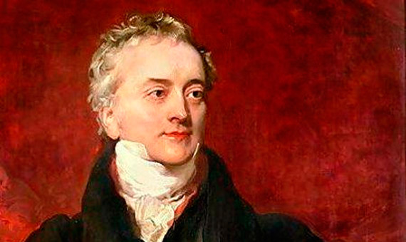
1. Thomas Young Polymath: The Law of Interference

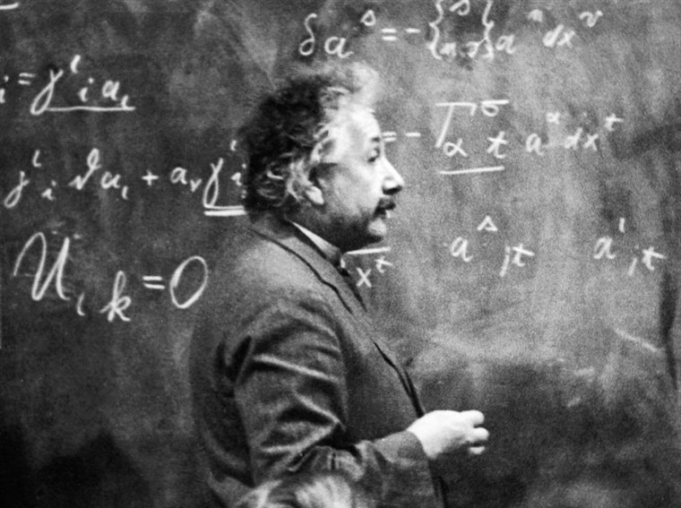
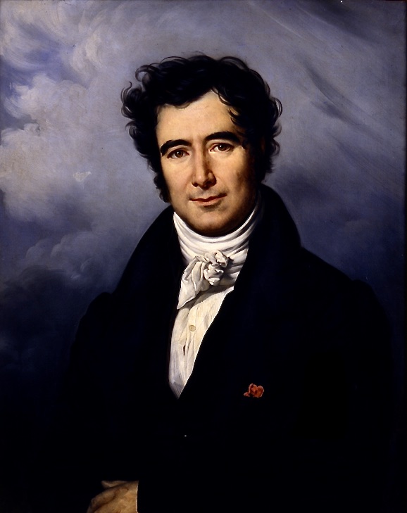
Thomas Young was the ultimate dabbler, his interests and explorations ranged far and wide, from ancient egyptology to naval engineering, from physiology of perception to the physics of sound and light. Yet unlike most dabblers who accomplish little, he made original and seminal contributions to all these fields. Some have called him the “Last Man Who Knew Everything“.

Topics: The Law of Interference. The Rosetta Stone. Benjamin Thompson, Count Rumford. Royal Society. Christiaan Huygens. Pendulum Clocks. Icelandic Spar. Huygens’ Principle. Stellar Aberration. Speed of Light. Double-slit Experiment.

1629 – Huygens born (1629 – 1695)

1642 – Galileo dies, Newton born (1642 – 1727)

1655 – Huygens ring of Saturn

1657 – Huygens patents the pendulum clock

1666 – Newton prismatic colors

1666 – Huygens moves to Paris

1669 – Bartholin double refraction in Icelandic spar

1670 – Bartholinus polarization of light by crystals

1671 – Expedition to Hven by Picard and Rømer

1673 – James Gregory bird-feather diffraction grating

1673 – Huygens publishes Horologium Oscillatorium

1675 – Rømer finite speed of light

1678 – Huygens and two crystals of Icelandic spar

1681 – Huygens returns to the Hague

1689 – Huyens meets Newton

1690 – Huygens Traite de la Lumiere

1695 – Huygens dies

1704 – Newton’s Opticks

1727 – Bradley abberation of starlight

1746 – Euler Nova theoria lucis et colorum

1773 – Thomas Young born

1786 – François Arago born (1786 – 1853)

1787 – Joseph Fraunhofer born (1787 – 1826)

1788 – Fresnel born in Broglie, Normandy (1788 – 1827)

1794 – École Polytechnique founded in Paris by Lazar Carnot and Gaspard Monge, Malus enters the Ecole

1794 – Young elected member of the Royal Society

1794 – Young enters Edinburg (cannot attend British schools because he was Quaker)

1795 – Young enters Göttingen

1796 – Young receives doctor of medicine, grand tour of Germany

1797 – Young returns to England, enters Emmanual College (converted to Church of England)

1798 – The Directory approves Napoleon’s Egyptian campaign, Battle of the Pyramids, Battle of the Nile

1799 – Young graduates from Cambridge

1799 – Royal Institution founded

1799 – Young Outlines

1800 – Young Sound and Light read to Royal Society,

1800 – Young Mechanisms of the Eye (Bakerian Lecture of the Royal Society)

1801 – Young Theory of Light and Colours, three color mechanism (Bakerian Lecture), Young considers interference to cause the colored films, first estimates of the wavelengths of different colors

1802 – Young begins series of lecturs at the Royal Institution (Jan. 1802 – July 1803)

1802 – Young names the principle (Law) of interference

1803 – Young’s 3^rd Bakerian Lecture, November. Experiments and Calculations Relative Physical to Optics, The Law of Interference

1807 – Young publishes A course of lectures on Natural Philosophy and the Mechanical Arts, based on Royal Institution lectures, two-slit experiment described

1808 – Malus polarization

1811 – Young appointed to St. Georges hospital

1813 – Young begins work on Rosetta stone

1814 – Young translates the demotic script on the stone

1816 – Arago visits Young

1818 – Young’s Encyclopedia article on Egypt

1822 – Champollion publishes translation of hieroglyphics

1827 – Young elected foreign member of the Institute of Paris

1829 – Young dies

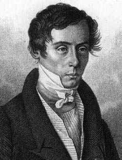
2. The Fresnel Connection: Particles versus Waves

Augustin Fresnel was an intuitive genius whose talents were almost squandered on his job building roads and bridges in the backwaters of France until he was discovered and rescued by Francois Arago.

Topics: Particles versus Waves. Malus and Polarization. Agustin Fresnel. Francois Arago. Diffraction. Daniel Bernoulli. The Principle of Superposition. Joseph Fourier. Transverse Light Waves.

1665 – Grimaldi diffraction bands outside shadow

1673 – James Gregory bird-feather diffraction grating

1675 – Römer finite speed of light

1704 – Newton’s Optics

1727 – Bradley abberation of starlight

1774 – Jean-Baptiste Biot born

1786 – David Rittenhouse hairs-on-screws diffraction grating

1786 – François Arago born (1786 – 1853)

1787 – Fraunhofer born (1787 – 1826)

1788 – Fresnel born in Broglie, Normandy (1788 – 1827)

1790 – Fresnel moved to Cherbourg

1794 – École Polytechnique founded in Paris by Lazar Carnot and Gaspard Monge

1804 – Fresnel attends Ecole polytechnique in Paris at age 16

1806 – Fresnel graduated and attended the national school of bridges and highways

1808 – Malus polarization

1809 – Fresnel graduated from Les Ponts

1809 – Arago returns from captivity in Algiers

1811 – Arago publishes paper on particle theory of light

1811 – Arago optical ratotory activity (rotation)

1814 – Fraunhofer spectroscope (solar absorption lines)

1815 – Fresnel meets Arago in Paris on way home to Mathieu (for house arrest)

1815 – Fresnel first paper on wave properties of diffraction

1816 – Fresnel returns to Paris to demonstrate his experiments

1816 – Arago visits Young

1816 – Fresnel paper on interference as origin of diffraction

1817 – French Academy announces its annual prize competition: topic of diffraction

1817 – Fresnel invents and uses his “Fresnel Integrals”

1819 – Fresnel awarded French Academy prize for wave theory of diffraction

1819 – Arago and Fresnel transverse and circular (?) polarization

1821 – Fraunhofer diffraction grating

1821 – Fresnel light is ONLY transverse

1821 – Fresnel double refraction explanation

1823 – Fraunhofer 3200 lines per Paris inch

1826 – Publication of Fresnel’s award memoire

1827 – Death of Fresnel by tuberculosis

1840 – Ernst Abbe born (1840 – 1905)

1849 – Stokes distribution of secondary waves

1850 – Fizeau and Foucault speed of light experiments

3. At Light Speed

There is no question that Francois Arago was a swashbuckler. His life’s story reads like an adventure novel as he went from being marooned in hostile lands early in his career to becoming prime minister of France after the 1848 revolutions swept across Europe.

Topics: The Birth of Interferometry. Snell’s Law. Fresnel and Arago. The First Interferometer. Fizeau and Foucault. The Speed of Light. Ether Drag. Jamin Interferometer.

1671 – Expedition to Hven by Picard and Rømer

1704 – Newton’s Opticks

1729 – James Bradley observation of stellar aberration

1784 – John Michel dark stars

1804 – Young wave theory of light and ether

1808 – Malus discovery of polarization of reflected light

1810 – Arago search for ether drag

1813 – Fraunhofer dark lines in Sun spectrum

1819 – Fresnel’s double mirror

1820 – Oersted discovers electromagnetism

1821 – Faraday electromagnetic phenomena

1821 – Fresnel light purely transverse

1823 – Fresnel reflection and refraction based on boundary conditions of ether

1827 – Green mathematical analysis of electricity and magnetism

GreenEssayGoogle Download

1830 – Cauchy ether as elastic solid

1831 – Faraday electromagnetic induction

1831 – Cauchy ether drag

1831 – Maxwell born

1831 – Faraday electromagnetic induction

1834 – Lloyd’s mirror

1836 – Cauchy’s second theory of the ether

1838 – Green theory of the ether

1839 – Hamilton group velocity

1839 – MacCullagh properties of rotational ether

1839 – Cauchy ether with negative compressibility

1841 – Maxwell entered Edinburgh Academy (age 10) met P. G. Tait

1842 – Doppler effect

DopplerFarbigeLicht-3 Download

1845 – Faraday effect (magneto-optic rotation)

1846 – Haidinger fringes

1846 – Stokes’ viscoelastic theory of the ether

1847 – Maxwell entered Edinburgh University

1848 – Fizeau proposal of the Fizeau-Doppler effect

1849 – Fizeau speed of light

1850 – Maxwell at Cambridge, studied under Hopkins, also knew Stokes and Whewell

1852 – Michelson born Strelno, Prussia

1854 – Maxwell wins the Smith’s Prize (Stokes’ theorem was one of the problems)

1855 – Michelson’s immigrate to San Francisco through Panama Canal

1855 – Maxwell “On Faraday’s Line of Force”

1856 – Jamin interferometer

1856 – Thomson magneto-optics effects (of Faraday)

1857 – Clausius constructs kinetic theory, Mean molecular speeds

Clausius (1857)_Nature motion we call heat Download

1859 – Fizeau light in moving medium

1862 – Fizeau fringes

1865 – Maxwell “A Dynamical Theory of the Electromagnetic Field”

1867 – Thomson and Tait “Treatise on Natural Philosophy”

1867 – Thomson hydrodynamic vortex atom

1868 – Fizeau proposal for stellar interferometry

1870 – Maxwell introduced “curl”, “convergence” and “gradient”

1871 – Maxwell appointed to Cambridge

1873 – Maxwell “A Treatise on Electricity and Magnetism”

4. After the Gold Rush

No name is more closely connected to interferometry than that of Albert Michelson. He succeeded, sometimes at great personal cost, in launching interferometric metrology as one of the most important tools used by scientists today.

Albert A. Michelson, 1907 Nobel Prize. Image Credit.

Topics: The Trials of Albert Michelson. Hermann von Helmholtz. Michelson and Morley. Fabry and Perot.

1810 – Arago search for ether drag

1813 – Fraunhofer dark lines in Sun spectrum

1813 – Faraday begins at Royal Institution

1820 – Oersted discovers electromagnetism

1821 – Faraday electromagnetic phenomena

1827 – Green mathematical analysis of electricity and magnetism

1830 – Cauchy ether as elastic solid

1831 – Faraday electromagnetic induction

1831 – Cauchy ether drag

1831 – Maxwell born

1831 – Faraday electromagnetic induction

1836 – Cauchy’s second theory of the ether

1838 – Green theory of the ether

1839 – Hamilton group velocity

1839 – MacCullagh properties of rotational ether

1839 – Cauchy ether with negative compressibility

1841 – Maxwell entered Edinburgh Academy (age 10) met P. G. Tait

1842 – Doppler effect

1845 – Faraday effect (magneto-optic rotation)

1846 – Stokes’ viscoelastic theory of the ether

1847 – Maxwell entered Edinburgh University

1850 – Maxwell at Cambridge, studied under Hopkins, also knew Stokes and Whewell

1852 – Michelson born Strelno, Prussia

1854 – Maxwell wins the Smith’s Prize (Stokes’ theorem was one of the problems)

1855 – Michelson’s immigrate to San Francisco through Panama Canal

1855 – Maxwell “On Faraday’s Line of Force”

1856 – Jamin interferometer

1856 – Thomson magneto-optics effects (of Faraday)

1859 – Fizeau light in moving medium

1859 – Discovery of the Comstock Lode

1860 – Maxwell publishes first paper on kinetic theory.

1861 – Maxwell “On Physical Lines of Force” speed of EM waves and molecular vortices, molecular vortex model

1862 – Michelson at boarding school in SF

1865 – Maxwell “A Dynamical Theory of the Electromagnetic Field”

1867 – Thomson and Tait “Treatise on Natural Philosophy”

1867 – Thomson hydrodynamic vortex atom

1868 – Fizeau proposal for stellar interferometry

1869 – Michelson meets US Grant and obtained appointment to Annapolis

1870 – Maxwell introduced “curl”, “convergence” and “gradient”

1871 – Maxwell appointed to Cambridge

1873 – Big Bonanza at the Consolidated Virginia mine

1873 – Maxwell “A Treatise on Electricity and Magnetism”

1873 – Michelson graduates from Annapolis

1875 – Michelson instructor at Annapolis

1877 – Michelson married Margaret Hemingway

1878 – Michelson First measurement of the speed of light with funds from father in law

1879 – Michelson Begin collaborating with Newcomb

1879 – Maxwell proposes second-order effect for ether drift experiments

1879 – Maxwell dies

1880 – Michelson Idea for second-order measurement of relative motion against ether

1880 – Michelson studies in Europe with Helmholtz in Berlin

1881 – Michelson Measurement at Potsdam with funds from Alexander Graham Bell

1882 – Michelson in Paris, Cornu, Mascart and Lippman

1882 – Michelson Joined Case School of Applied Science

1884 – Poynting energy flux vector

1885 – Michelson Began collaboration with Edward Morley of Western Reserve

1885 – Lorentz points out inconsistency of Stokes’ ether model

1885 – Fitzgerald wheel and band model, vortex sponge

1886 – Michelson and Morley repeat the Fizeau moving water experiment

Michelson1886 Download

1887 – Michelson Five days in July experiment on motion relative to ether

1887 – Michelson-Morley experiment published

MichelsonMorley1887 Download

1887 – Voigt derivation of relativistic Doppler (with coordinate transformations)

Voigt1887 Download

1888 – Hertz generation and detection of radio waves

1889 – Michelson moved to Clark University at Worcester

1889 – Fitzgerald contraction

1889 – Lodge cogwheel model of electromagnetism

1890 – Michelson Proposed use of interferometry in astronomy

1890 – Thomson devises a mechanical model of MacCullagh’s rotational ether

1890 – Hertz Galileo relativity and ether drag

1891 – Mach-Zehnder

1891 – Michelson measures diameter of Jupiter’s moons with interferometry

1891 – Thomson vortex electromagnetism

1892 – 1893 Michelson measurement of the Paris meter

1893 – Sirks interferometer

1893 – Michelson moved to University of Chicago to head Physics Dept.

1893 – Lorentz contraction

1894 – Lodge primitive radio demonstration

1895 – Marconi radio

1896 – Rayleigh’s interferometer

1897 – Lodge no ether drag on laboratory scale

1898 – Pringsheim interferometer

1899 – Fabry-Perot interferometer

1899 – Michelson remarried

1901 – 1903 Michelson President of the APS

1905 – Poincaré names the Lorentz transformations

1905 – Einstein’s special theory of Relativity

1907 – Michelson Nobel Prize

1913 – Sagnac interferometer

1916 – Twyman-Green interferometer

1920 – Stellar interferometer on the Hooker 100-inch telescope (Betelgeuse)

1923 – 1927 Michelson presided over the National Academy of Sciences

1931 – Michelson dies

5. Stellar Interference

Learning from his attempts to measure the speed of light through the ether, Michelson realized that the partial coherence of light from astronomical sources could be used to measure their sizes. His first measurements using the Michelson Stellar Interferometer launched a major subfield of astronomy that is one of the most active today.

Topics: Measuring the Stars. Astrometry. Moons of Jupiter. Schwarzschild. Betelgeuse. Michelson Stellar Interferometer. Banbury Brown Twiss. Sirius. Adaptive Optics.

1838 – Bessel stellar parallax measurement with Fraunhofer telescope

1868 – Fizeau proposes stellar interferometry

1873 – Stephan implements Fizeau’s stellar interferometer on Sirius, sees fringes

1880 – Michelson Idea for second-order measurement of relative motion against ether

1880 – 1882 Michelson Studies in Europe (Helmholtz in Berlin, Quincke in Heidelberg, Cornu, Mascart and Lippman in Paris)

1881 – Michelson Measurement at Potsdam with funds from Alexander Graham Bell

1881 – Michelson Resigned from active duty in the Navy

1883 – Michelson Joined Case School of Applied Science

1889 – Michelson moved to Clark University at Worcester

1890 – Michelson develops mathematics of stellar interferometry

1891 – Michelson measures diameters of Jupiter’s moons

Michelson1891 Download

1893 – Michelson moves to University of Chicago to head Physics Dept.

1896 – Schwarzschild double star interferometry

1907 – Michelson Nobel Prize

1908 – Hale uses Zeeman effect to measure sunspot magnetism

1910 – Taylor single-photon double slit experiment

1915 – Proxima Centauri discovered by Robert Innes

1916 – Einstein predicts gravitational waves

1920 – Stellar interferometer on the Hooker 100-inch telescope (Betelgeuse)

Michelson1921 Download

1947 – McCready sea interferometer observes rising sun (first fringes in radio astronomy

1952 – Ryle radio astronomy long baseline

1954 – Hanbury-Brown and Twiss radio intensity interferometry

1956 – Hanbury-Brown and Twiss optical intensity correlation, Sirius (optical)

1958 – Jennison closure phase

1970 – Labeyrie speckle interferometry

1974 – Long-baseline radio interferometry in practice using closure phase

1974 – Johnson, Betz and Townes: IR long baseline

1975 – Labeyrie optical long-baseline

1982 – Fringe measurements at 2.2 microns Di Benedetto

1985 – Baldwin closure phase at optical wavelengths

1991 – Coude du Foresto single-mode fibers with separated telescopes

1993 – Nobel prize to Hulse and Taylor for binary pulsar

1995 – Baldwin optical synthesis imaging with separated telescopes

1991 – Mayor and Queloz Doppler pull of 51 Pegasi

1999 – Upsilon Andromedae multiple planets

2009 – Kepler space telescope launched

2014 – Kepler announces 715 planets

2015 – Kepler-452b Earthlike planet in habitable zone

2015 – First detection of gravitational waves

2016 – Proxima Centauri b exoplanet confirmed

2017 – Nobel prize for gravitational waves

2018 – TESS (Transiting Exoplanet Survey Satellite)

2019 – Mayor and Queloz win Nobel prize for first exoplanet

2019 – First direct observation of exoplanet using interferometry

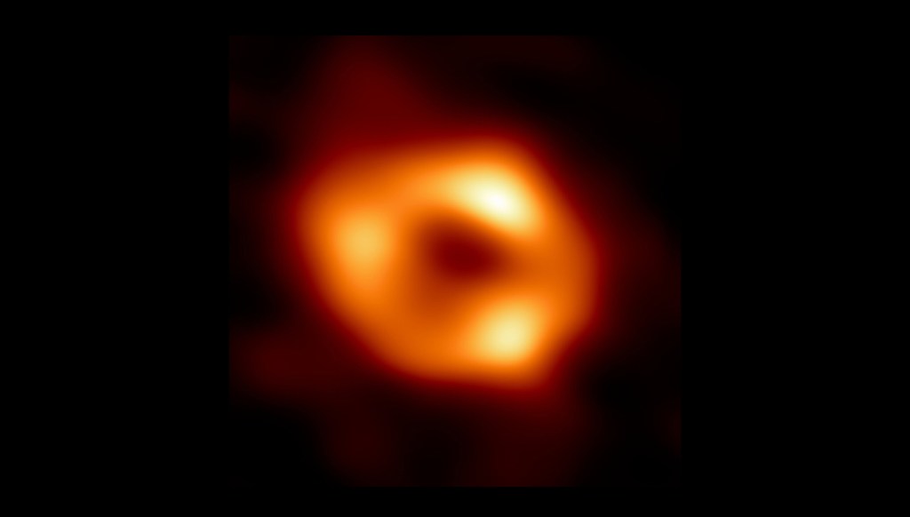
2019 – First image of a black hole obtained by very-long-baseline interferometry

6. Across the Universe

Stellar interferometry is opening new vistas of astronomy, exploring the wildest occupants of our universe, from colliding black holes half-way across the universe (LIGO) to images of neighboring black holes (EHT) to exoplanets near Earth that may harbor life.

Image of the supermassive black hole in M87 from Event Horizon Telescope.

Topics: Gravitational Waves, Black Holes and the Search for Exoplanets. Nulling Interferometer. Event Horizon Telescope. M87 Black Hole. Long Baseline Interferometry. LIGO.

1947 – Virgo A radio source identified as M87

1953 – Horace W. Babcock proposes adaptive optics (AO)

Babcock1953 Download

1958 – Jennison closure phase

1967 – First very long baseline radio interferometers (from meters to hundreds of km to thousands of km within a single year)

1967 – Ranier Weiss begins first prototype gravitational wave interferometer

1967 – Virgo X-1 x-ray source (M87 galaxy)

1970 – Poul Anderson’s Tau Zero alludes to AO in science fiction novel

1973 – DARPA launches adaptive optics research with contract to Itek, Inc.

1974 – Wyant (Itek) white-light shearing interferometer

1974 – Long-baseline radio interferometry in practice using closure phase

1975 – Hardy (Itek) patent for adaptive optical system

1975 – Weiss funded by NSF to develop interferometer for GW detection

1977 – Demonstration of AO on Sirius (Bell Labs and Berkeley)

1980 – Very Large Array (VLA) 6 mm to 4 meter wavelengths

1981 – Feinleib proposes atmospheric laser backscatter

1982 – Will Happer at Princeton proposes sodium guide star

1982 – Fringe measurements at 2.2 microns (Di Benedetto)

1983 – Sandia Optical Range demonstrates artificial guide star (Rayleigh)

1983 – Strategic Defense Initiative (Star Wars)

1984 – Lincoln labs sodium guide star demo

1984 – ESO plans AO for Very Large Telescope (VLT)

1985 – Laser guide star (Labeyrie)

1985 – Closure phase at optical wavelengths (Baldwin)

1988 – AFWL names Starfire Optical Range, Kirtland AFB outside Albuquerque

1988 – Air Force Maui Optical Site Schack-Hartmann and 241 actuators (Itek)

1988 – First funding for LIGO feasibility

1989 – 19-element-mirror Double star on 1.5m telescope in France

1989 – VLT approved for construction

1990 – Launch of the Hubble Space Telescope

1991 – Single-mode fibers with separated telescopes (Coude du Foresto)

1992 – ADONIS

1992 – NSF requests declassification of AO

1993 – VLBA (Very Long Baseline Array) 8,611 km baseline 3 mm to 90 cm

1994 – Declassification completed

1994 – Curvature sensor 3.6m Canada-France-Hawaii

1994 – LIGO funded by NSF, Barish becomes project director

1995 – Optical synthesis imaging with separated telescopes (Baldwin)

1995 – Doppler pull of 51 Pegasi (Mayor and Queloz)

1998 – ESO VLT first light

1998 – Keck installed with Schack-Hartmann

1999 – Upsilon Andromedae multiple planets

2000 – Hale 5m Palomar Schack-Hartmann

2001 – NAOS-VLT adaptive optics

2001 – VLTI first light (MIDI two units)

2002 – LIGO operation begins

2007 – VLT laser guide star

2007 – VLTI AMBER first scientific results (3 units)

2009 – Kepler space telescope launched

2009 – Event Horizon Telescope (EHT) project starts

2010 – Large Binocular Telescope (LBT) 672 actuators on secondary mirror

2010 – End of first LIGO run. No events detected. Begin Enhanced LIGO upgrade.

2011 – SPHERE-VLT 41×41 actuators (1681)

2012 – Extremely Large Telescope (ELT) approved for construction

2014 – Kepler announces 715 planets

2015 – Kepler-452b Earthlike planet in habitable zone

2015 – First detection of gravitational waves (LIGO)

2015 – LISA Pathfinder launched

2016 – Second detection at LIGO

2016 – Proxima Centauri b exoplanet confirmed

2016 – GRAVITY VLTI (4 units)

2017 – Nobel prize for gravitational waves

2018 – TESS (Transiting Exoplanet Survey Satellite) launched

2018 – MATTISE VLTI first light (combining all units)

2019 – Mayor and Queloz win Nobel prize

2019 – First direct observation of exoplanet using interferometry at LVTI

2019 – First image of a black hole obtained by very-long-baseline interferometry (EHT)

2020 – First neutron-star black-hole merger detected

2020 – KAGRA (Japan) online

2024 – LIGO India to go online

2025 – First light for ELT

2034 – Launch date for LISA

7. Two Faces of Microscopy

From the astronomically large dimensions of outer space to the microscopically small dimensions of inner space, optical interference pushes the resolution limits of imaging.

Topics: Diffraction and Interference. Joseph Fraunhofer. Diffraction Gratings. Henry Rowland. Carl Zeiss. Ernst Abbe. Phase-contrast Microscopy. Super-resolution Micrscopes. Structured Illumination.

1021 – Al Hazeni manuscript on Optics

1284 – First eye glasses by Salvino D’Armate

1590 – Janssen first microscope

1609 – Galileo first compound microscope

1625 – Giovanni Faber coins phrase “microscope”

1665 – Hook’s Micrographia

1676 – Antonie van Leeuwenhoek microscope

1787 – Fraunhofer born

1811 – Fraunhofer enters business partnership with Utzschneider

1816 – Carl Zeiss born

1821 – Fraunhofer first diffraction publication

1823 – Fraunhofer second diffraction publication 3200 lines per Paris inch

1830 – Spherical aberration compensated by Joseph Jackson Lister

1840 – Ernst Abbe born

1846 – Zeiss workshop in Jena, Germany

1850 – Fizeau and Foucault speed of light

1851 – Otto Schott born

1859 – Kirchhoff and Bunsen theory of emission and absorption spectra

1866 – Abbe becomes research director at Zeiss

1874 – Ernst Abbe equation on microscope resolution

1874 – Helmholtz image resolution equation

1880 – Rayleigh resolution

1888 – Hertz waves

1888 – Frits Zernike born

1925 – Zsigmondy Nobel Prize for light-sheet microscopy

1931 – Transmission electron microscope by Ruske and Knoll

1932 – Phase contrast microscope by Zernicke

1942 – Scanning electron microscope by Ruska

1949 – Mirau interferometric objective

1952 – Nomarski differential phase contrast microscope

1953 – Zernicke Nobel prize

1955 – First discussion of superresolution by Toraldo di Francia

1957 – Marvin Minsky patents confocal principle

1962 – Green flurescence protein (GFP) Shimomura, Johnson and Saiga

1966 – Structured illumination microscopy by Lukosz

1972 – CAT scan

1978 – Cremer confocal laser scanning microscope

1978 – Lohman interference microscopy

1981 – Binnig and Rohrer scanning tunneling microscope (STM)

1986 – Microscopy Nobel Prize: Ruska, Binnig and Rohrer

1990 – 4PI microscopy by Stefan Hell

1992 – GFP cloned

1993 – STED by Stefan Hell

1993 – Light sheet fluorescence microscopy by Spelman

1995 – Structured illumination microscopy by Guerra

1995 – Gustafsson image interference microscopy

1999 – Gustafsson I⁵M

2004 – Selective plane illumination microscopy (SPIM)

2006 – PALM and STORM (Betzig and Zhuang)

2014 – Nobel Prize (Hell, Betzig and Moerner)

8. Holographic Dreams of Princess Leia

The coherence of laser light is like a brilliant jewel that sparkles in the darkness, illuminating life, probing science and projecting holograms in virtual worlds.

Topics: Crossing Beams. Denis Gabor. Wavefront Reconstruction. Holography. Emmett Leith. Lasers. Ted Maiman. Charles Townes. Optical Maser. Dynamic Holography. Light-field Imaging.

1900 – Dennis Gabor born

1926 – Hans Busch magnetic electron lens

1927 – Gabor doctorate

1931 – Ruska and Knoll first two-stage electron microscope

1942 – Lawrence Bragg x-ray microscope

1948 – Gabor holography paper in Nature

1949 – Gabor moves to Imperial College

1950 – Lamb possibility of population inversion

1951 – Purcell and Pound demonstration of population inversion

1952 – Leith joins Willow Run Labs

1953 – Townes first MASER

1957 – SAR field trials

1957 – Gould coins LASER

1958 – Schawlow and Townes proposal for optical maser

1959 – Shawanga Lodge conference

1960 – Maiman first laser: pink ruby

1960 – Javan first gas laser: HeNe at 1.15 microns

1961 – Leith and Upatnieks wavefront reconstruction

1962 – HeNe laser in the visible at 632.8 nm

1962 – First laser holograms (Leith and Upatnieks)

1963 – van Heerden optical information storage

1963 – Leith and Upatnieks 3D holography

1966 – Ashkin optically-induced refractive index changes

1966 – Leith holographic information storage in 3D

1968 – Bell Labs holographic storage in Lithium Niobate and Tantalate

1969 – Kogelnik coupled wave theory for thick holograms

1969 – Electrical control of holograms in SBN

1970 – Optically induced refractive index changes in Barium Titanate

1971 – Amodei transport models of photorefractive effect

1971 – Gabor Nobel prize

1972 – Staebler multiple holograms

1974 – Glass and von der Linde photovoltaic and photorefractive effects, UV erase

1977 – Star Wars movie

1981 – Huignard two-wave mixing energy transfer

2012 – Coachella Music Festival

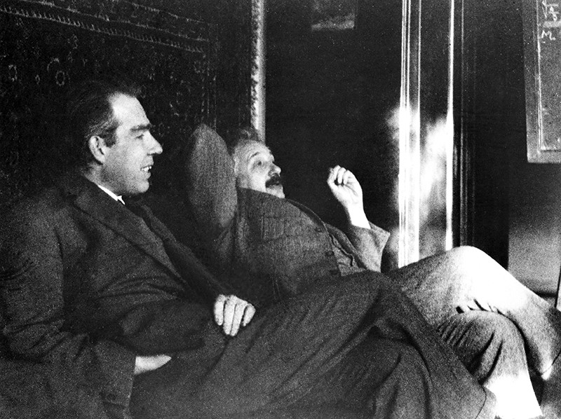
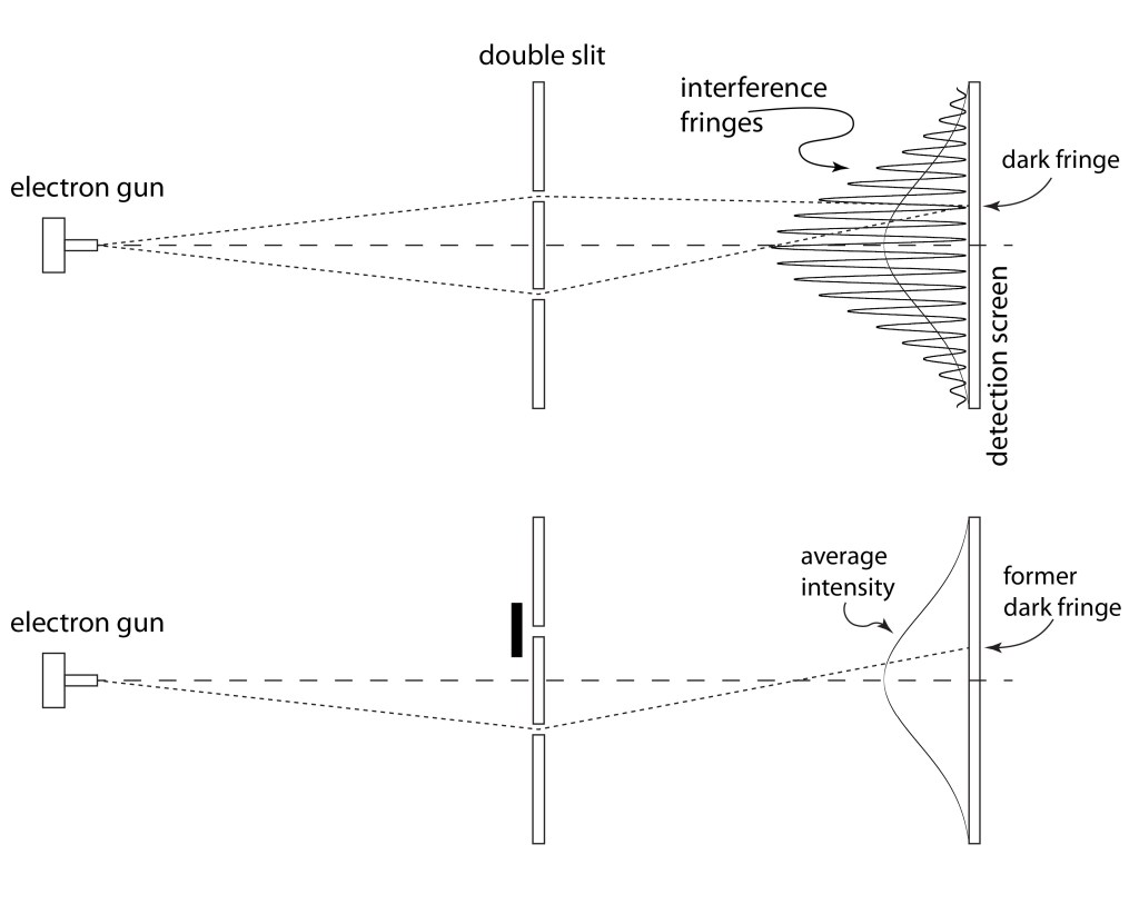
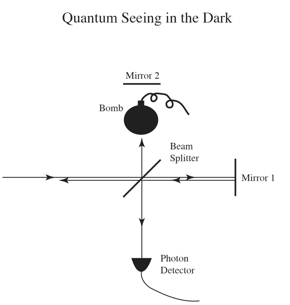
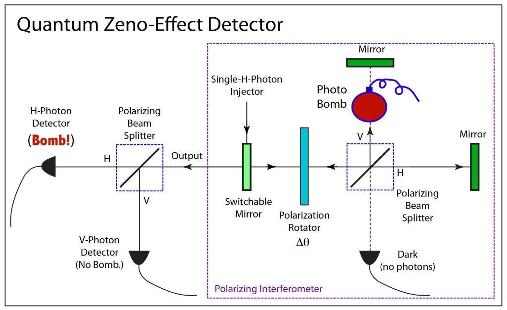
9. Photon Interference

What is the image of one photon interfering? Better yet, what is the image of two photons interfering? The answer to this crucial question laid the foundation for quantum communication.

Topics: The Beginnings of Quantum Communication. EPR paradox. Entanglement. David Bohm. John Bell. The Bell Inequalities. Leonard Mandel. Single-photon Interferometry. HOM Interferometer. Two-photon Fringes. Quantum cryptography. Quantum Teleportation.

1900 – Planck (1901). “Law of energy distribution in normal spectra.” [1]

Planck-1901-Annalen_der_Physik Download

1905 – A. Einstein (1905). “Generation and conversion of light wrt a heuristic point of view.” [2]

1909 – A. Einstein (1909). “On the current state of radiation problems.” [3]

1909 – Single photon double-slit experiment, G.I. Taylor [4]

1915 – Milliken photoelectric effect

1916 – Einstein predicts stimulated emission

1923 –Compton, Arthur H. (May 1923). Quantum Theory of the Scattering of X-Rays.[5]

1926 – Gilbert Lewis names “photon”

1926 – Dirac: photons interfere only with themselves

1927 – D. Dirac, P. A. M. (1927). Emission and absorption of radiation [6]

1932 – von Neumann textbook on quantum physics

1932 – E. P. Wigner: Phys. Rev. 40, 749 (1932)

1935 – EPR paper, A. Einstein, B. Podolsky, N. Rosen: Phys. Rev. 47 , 777 (1935)

1935 – Reply to EPR, N. Bohr: Phys. Rev. 48 , 696 (1935)

1935 – Schrödinger (1935 and 1936) on entanglement (cat?) “Present situation in QM”

1948 – Gabor holography

1950 – Wu correlated spin generation from particle decay

1951 – Bohm alternative form of EPR gedankenexperiment (quantum textbook)

1952 – Bohm nonlocal hidden variable theory[7]

1953 – Schwinger: Coherent states

1956 – Photon bunching, R. Hanbury-Brown, R.W. Twiss: Nature 177 , 27 (1956)

1957 – Bohm and Ahronov proof of entanglement in 1950 Wu experiment

1959 – Ahronov-Bohm effect of magnetic vector potential

1960 – Klauder: Coherent states

1963 – Coherent states, R. J. Glauber: Phys. Rev. 130 , 2529 (1963)

1963 – Coherent states, E. C. G. Sudarshan: Phys. Rev. Lett. 10, 277 (1963)

1964 – J. S. Bell: Bell inequalities [8]

1964 – Mandel professorship at Rochester

1967 – Interference at single photon level, R. F. Pfleegor, L. Mandel: [9]

1967 – M. O. Scully, W.E. Lamb: Phys. Rev. 159 , 208 (1967) Quantum theory of laser

1967 – Parametric converter (Mollow and Glauber) [10]

1967 – Kocher and Commins calcium 2-photon cascade

1969 – Quantum theory of laser, M. Lax, W.H. Louisell: Phys. Rev. 185 , 568 (1969)

1969 – CHSH inequality [11]

1972 – First test of Bell’s inequalities (Freedman and Clauser)

1975 – Carmichel and Walls predicted light in resonance fluorescence from a two-level atom would display photon anti-bunching (1976)

1977 – Photon antibunching in resonance fluorescence. H. J. Kimble, M. Dagenais and L. Mandel [12]

1978 – Kip Thorne quantum non-demolition (QND)

1979 – Hollenhorst squeezing for gravitational wave detection: names squeezing

1982 – Apect Experimental Bell experiments, [13]

1985 – Dick Slusher experimental squeezing

1985 – Deutsch quantum algorithm

1986 – Photon anti-bunching at a beamsplitter, P. Grangier, G. Roger, A. Aspect: [14]

1986 – Kimble squeezing in parametric down-conversion

1986 – C. K. Hong, L. Mandel: Phys. Rev. Lett. 56 , 58 (1986) one-photon localization

1987 – Two-photon interference (Ghosh and Mandel) [15]

1987 – HOM effect [16]

1987 – Photon squeezing, P. Grangier, R. E. Slusher, B. Yurke, A. La Porta: [17]

1987 – Grangier and Slusher, squeezed light interferometer

1988 – 2-photon Bell violation: Z. Y. Ou, L. Mandel: Phys. Rev. Lett. 61 , 50 (1988)

1988 – Brassard Quantum cryptography

1989 – Franson proposes two-photon interference in k-number (?)

1990 – Two-photon interference in k-number (Kwiat and Chiao)

1990 – Two-photon interference (Ou, Zhou, Wang and Mandel)

1993 – Quantum teleportation proposal (Bennett)

1994 – Teleportation of quantum states (Vaidman)

1994 – Shor factoring algorithm

1995 – Down-conversion for polarization: Kwiat and Zeilinger (1995)

1997 – Experimental quantum teleportation (Bouwmeester)

1997 – Experimental quantum teleportation (Bosci)

1998 – Unconditional quantum teleportation (every state) (Furusawa)

2001 – Quantum computing with linear optics (Knill, Laflamme, Milburn)

2013 – LIGO design proposal with squeezed light (Aasi)

2019 – Squeezing upgrade on LIGO (Tse)

2020 – Quantum computational advantage (Zhong)

10. The Quantum Advantage

There is almost no technical advantage better than having exponential resources at hand. The exponential resources of quantum interference provide that advantage to quantum computing which is poised to usher in a new era of quantum information science and technology.

Topics: Interferometric Computing. David Deutsch. Quantum Algorithm. Peter Shor. Prime Factorization. Quantum Logic Gates. Linear Optical Quantum Computing. Boson Sampling. Quantum Computational Advantage.

1980 – Paul Benioff describes possibility of quantum computer

1981 – Feynman simulating physics with computers

1985 – Deutsch quantum Turing machine [18]

1987 – Quantum properties of beam splitters

1992 – Deutsch Josza algorithm is exponential faster than classical

1993 – Quantum teleportation described

1994 – Shor factoring algorithm [19]

1994 – First quantum computing conference

1995 – Shor error correction

1995 – Universal gates

1996 – Grover search algorithm

1998 – First demonstration of quantum error correction

1999 – Nakamura and Tsai superconducting qubits

2001 – Superconducting nanowire photon detectors

2001 – Linear optics quantum computing (KLM)

2001 – One-way quantum computer

2003 – All-optical quantum gate in a quantum dot (Li)

2003 – All-optical quantum CNOT gate (O’Brien)

2003 – Decoherence and einselection (Zurek)

2004 – Teleportation across the Danube

2005 – Experimental quantum one-way computing (Walther)

2007 – Teleportation across 114 km (Canary Islands)

2008 – Quantum discord computing

2011 – D-Wave Systems offers commercial quantum computer

2011 – Aaronson boson sampling

2012 – 1QB Information Technnologies, first quantum software company

2013 – Experimental demonstrations of boson sampling

2014 – Teleportation on a chip

2015 – Universal linear optical quantum computing (Carolan)

2017 – Teleportation to a satellite

2019 – Generation of a 2D cluster state (Larsen)

2019 – Quantum supremacy [20]

2020 – Quantum optical advantage [21]

2021 – Programmable quantum photonic chip

References:

[1] Annalen Der Physik 4(3): 553-563.

[2] Annalen Der Physik 17(6): 132-148.

[3] Physikalische Zeitschrift 10: 185-193.

[4] Proc. Cam. Phil. Soc. Math. Phys. Sci. 15 , 114 (1909)

[5] Physical Review. 21 (5): 483–502.

[6] Proceedings of the Royal Society of London Series a-Containing Papers of a Mathematical and Physical Character 114(767): 243-265.

[7] D. Bohm, “A suggested interpretation of the quantum theory in terms of hidden variables .1,” Physical Review, vol. 85, no. 2, pp. 166-179, (1952)

[8] Physics 1 , 195 (1964); Rev. Mod. Phys. 38 , 447 (1966)

[9] Phys. Rev. 159 , 1084 (1967)

[10] B. R. Mollow, R. J. Glauber: Phys. Rev. 160, 1097 (1967); 162, 1256 (1967)

[11] J. F. Clauser, M. A. Horne, A. Shimony, and R. A. Holt, ” Proposed experiment to test local hidden-variable theories,” Physical Review Letters, vol. 23, no. 15, pp. 880-&, (1969)

[12] (1977) Phys. Rev. Lett. 39, 691-5

[13] A. Aspect, P. Grangier, G. Roger: Phys. Rev. Lett. 49 , 91 (1982). A. Aspect, J. Dalibard, G. Roger: Phys. Rev. Lett. 49 , 1804 (1982)

[14] Europhys. Lett. 1 , 173 (1986)

[15] R. Ghosh and L. Mandel, “Observation of nonclassical effects in the interference of 2 photons,” Physical Review Letters, vol. 59, no. 17, pp. 1903-1905, Oct (1987)

[16] C. K. Hong, Z. Y. Ou, and L. Mandel, “Measurement of subpicosecond time intervals between 2 photons by interference,” Physical Review Letters, vol. 59, no. 18, pp. 2044-2046, Nov (1987)

[17] Phys. Rev. Lett 59, 2153 (1987)

[18] D. Deutsch, “QUANTUM-THEORY, THE CHURCH-TURING PRINCIPLE AND THE UNIVERSAL QUANTUM COMPUTER,” Proceedings of the Royal Society of London Series a-Mathematical Physical and Engineering Sciences, vol. 400, no. 1818, pp. 97-117, (1985)

[19] P. W. Shor, “ALGORITHMS FOR QUANTUM COMPUTATION – DISCRETE LOGARITHMS AND FACTORING,” in 35th Annual Symposium on Foundations of Computer Science, Proceedings, S. Goldwasser Ed., (Annual Symposium on Foundations of Computer Science, 1994, pp. 124-134.

[20] F. Arute et al., “Quantum supremacy using a programmable superconducting processor,” Nature, vol. 574, no. 7779, pp. 505-+, Oct 24 (2019)

[21] H.-S. Zhong et al., “Quantum computational advantage using photons,” Science, vol. 370, no. 6523, p. 1460, (2020)

The Many Worlds of the Quantum Beam Splitter

In one interpretation of quantum physics, when you snap your fingers, the trajectory you are riding through reality fragments into a cascade of alternative universes—one for each possible quantum outcome among all the different quantum states composing the molecules of your fingers.

This is the Many-Worlds Interpretation (MWI) of quantum physics first proposed rigorously by Hugh Everett in his doctoral thesis in 1957 under the supervision of John Wheeler at Princeton University. Everett had been drawn to this interpretation when he found inconsistencies between quantum physics and gravitation—topics which were supposed to have been his actual thesis topic. But his side-trip into quantum philosophy turned out to be a one-way trip. The reception of his theory was so hostile, no less than from Copenhagen and Bohr himself, that Everett left physics and spent a career at the Pentagon.

Resurrecting MWI in the Name of Quantum Information

Fast forward by 20 years, after Wheeler had left Princeton for the University of Texas at Austin, and once again a young physicist was struggling to reconcile quantum physics with gravity. Once again the many worlds interpretation of quantum physics seemed the only sane way out of the dilemma, and once again a side-trip became a life-long obsession.

David Deutsch, visiting Wheeler in the early 1980’s, became convinced that the many worlds interpretation of quantum physics held the key to paradoxes in the theory of quantum information (For the full story of Wheeler, Everett and Deutsch, see Ref [1]). He was so convinced, that he began a quest to find a physical system that operated on more information than could be present in one universe at a time. If such a physical system existed, it would be because streams of information from more than one universe were coming together and combining in a way that allowed one of the universes to “borrow” the information from the other.

It took only a year or two before Deutsch found what he was looking for—a simple quantum algorithm that yielded twice as much information as would be possible if there were no parallel universes. This is the now-famous Deutsch algorithm—the first quantum algorithm [2]. At the heart of the Deutsch algorithm is a simple quantum interference. The algorithm did nothing useful—but it convinced Deutsch that two universes were interfering coherently in the measurement process, giving that extra bit of information that should not have been there otherwise. A few years later, the Deutsch-Josza algorithm [2] expanded the argument to interfere an exponentially larger amount of information streams from an exponentially larger number of universes to create a result that was exponentially larger than any classical computer could produce. This marked the beginning of the quest for the quantum computer that is running red-hot today.

Deutsch’s “proof” of the many-worlds interpretation of quantum mechanics is not a mathematical proof but is rather a philosophical proof. It holds no sway over how physicists do the math to make their predictions. The Copenhagen interpretation, with its “spooky” instantaneous wavefunction collapse, works just fine predicting the outcome of quantum algorithms and the exponential quantum advantage of quantum computing. Therefore, the story of David Deutsch and the MWI may seem like a chimera—except for one fact—it inspired him to generate the first quantum algorithm that launched what may be the next revolution in the information revolution of modern society. Inspiration is important in science, because it lets scientists create things that had been impossible before.

But if quantum interference is the heart of quantum computing, then there is one physical system that has the ultimate simplicity that may yet inspire future generations of physicists to invent future impossible things—the quantum beam splitter. Nothing in the study of quantum interference can be simpler than a sliver of dielectric material sending single photons one way or another. Yet the outcome of this simple system challenges the mind and reminds us of why Everett and Deutsch embraced the MWI in the first place.

The Classical Beam Splitter

The so-called “beam splitter” is actually a misnomer. Its name implies that it takes a light beam and splits it into two, as if there is only one input. But every “beam splitter” has two inputs, which is clear by looking at the classical 50/50 beam splitter. The actual action of the optical element is the combination of beams into superpositions in each of the outputs. It is only when one of the input fields is zero, a special case, that the optical element acts as a beam splitter. In general, it is a beam combiner.

Given two input fields, the output fields are superpositions of the inputs

The square-root of two factor ensures that energy is conserved, because optical fluence is the square of the fields. This relation is expressed more succinctly as a matrix input-output relation

The phase factors in these equations ensure that the matrix is unitary

reflecting energy conservation.

The Quantum Beam Splitter

A quantum beam splitter is just a classical beam splitter operating at the level of individual photons. Rather than describing single photons entering or leaving the beam splitter, it is more practical to describe the properties of the fields through single-photon quantum operators

where the unitary matrix is the same as the classical case, but with fields replaced by the famous “a” operators. The photon operators operate on single photon modes. For instance, the two one-photon input cases are

where the creation operators operate on the vacuum state in each of the input modes.

The fundamental combinational properties of the beam splitter are even more evident in the quantum case, because there is no such thing as a single input to a quantum beam splitter. Even if no photons are directed into one of the input ports, that port still receives a “vacuum” input, and this vacuum input contributes to the fluctuations observed in the outputs.

The input-output relations for the quantum beam splitter are

The beam splitter operating on a one-photon input converts the input-mode creation operator into a superposition of out-mode creation operators that generates

The resulting output is entangled: either the single photon exits one port, or it exits the other. In the many worlds interpretation, the photon exits from one port in one universe, and it exits from the other port in a different universe. On the other hand, in the Copenhagen interpretation, the two output ports of the beam splitter are perfectly anti-correlated.

Fig. 1 Quantum Operations of a Beam Splitter. A beam splitter creates a quantum superposition of the input modes. The a-symbols are quantum number operators that create and annihilate photons. A single-photon input produces an entangled output that is a quantum superposition of the photon coming out of one output or the other.

The Hong-Ou-Mandel (HOM) Interferometer

When more than one photon is incident on a beam splitter, the fascinating effects of quantum interference come into play, creating unexpected outputs for simple inputs. For instance, the simplest example is a two photon input where a single photon is present in each input port of the beam splitter. The input state is represented with single creation operators operating on each vacuum state of each input port

creating a single photon in each of the input ports. The beam splitter operates on this input state by converting the input-mode creation operators into out-put mode creation operators to give

The important step in this process is the middle line of the equations: There is perfect destructive interference between the two single-photon operations. Therefore, both photons always exit the beam splitter from the same port—never split. Furthermore, the output is an entangled two-photon state, once more splitting universes.

Fig. 2 The HOM interferometer. A two-photon input on a beam splitter generates an entangled superposition of the two photons exiting the beam splitter always together.

The two-photon interference experiment was performed in 1987 by Chung Ki Hong and Jeff Ou, students of Leonard Mandel at the Optics Institute at the University of Rochester [4], and this two-photon operation of the beam splitter is now called the HOM interferometer. The HOM interferometer has become a center-piece for optical and photonic implementations of quantum information processing and quantum computers.

N-Photons on a Beam Splitter

Of course, any number of photons can be input into a beam splitter. For example, take the N-photon input state

The beam splitter acting on this state produces

The quantity on the right hand side can be re-expressed using the binomial theorem

where the permutations are defined by the binomial coefficient

The output state is given by

which is a “super” entangled state composed of N multi-photon states, involving N different universes.

Coherent States on a Quantum Beam Splitter

Surprisingly, there is a multi-photon input state that generates a non-entangled output—as if the input states were simply classical fields. These are the so-called coherent states, introduced by Glauber and Sudarshan [5, 6]. Coherent states can be described as superpositions of multi-photon states, but when a beam splitter operates on these superpositions, the outputs are simply 50/50 mixtures of the states. For instance, if the input scoherent tates are denoted by α and β, then the output states after the beam splitter are

This output is factorized and hence is NOT entangled. This is one of the many reasons why coherent states in quantum optics are considered the “most classical” of quantum states. In this case, a quantum beam splitter operates on the inputs just as if they were classical fields.

By David D. Nolte, May 8, 2022

References

[1] David D. Nolte, Interference: The History of Optical Interferometry and the Scientists who Tamed Light, (Oxford, July 2023)

[2] D. Deutsch, “Quantum-theory, the church-turing principle and the universal quantum computer,” Proceedings of the Royal Society of London Series a-Mathematical Physical and Engineering Sciences, vol. 400, no. 1818, pp. 97-117, (1985)

[3] D. Deutsch and R. Jozsa, “Rapid solution of problems by quantum computation,” Proceedings of the Royal Society of London Series a-Mathematical Physical and Engineering Sciences, vol. 439, no. 1907, pp. 553-558, Dec (1992)

[4] C. K. Hong, Z. Y. Ou, and L. Mandel, “Measurement of subpicosecond time intervals between 2 photons by interference,” Physical Review Letters, vol. 59, no. 18, pp. 2044-2046, Nov (1987)

[5] Glauber, R. J. (1963). “Photon Correlations.” Physical Review Letters 10(3): 84.

[6] Sudarshan, E. C. G. (1963). “Equivalence of semiclassical and quantum mechanical descriptions of statistical light beams.” Physical Review Letters 10(7): 277-&.; Mehta, C. L. and E. C. Sudarshan (1965). “Relation between quantum and semiclassical description of optical coherence.” Physical Review 138(1B): B274.

December 20, 2021October 23, 2023 by David D. Nolte

Twenty Years at Light Speed: The Future of Photonic Quantum Computing

Now is exactly the wrong moment to be reviewing the state of photonic quantum computing — the field is moving so rapidly, at just this moment, that everything I say here now will probably be out of date in just a few years. On the other hand, now is exactly the right time to be doing this review, because so much has happened in just the past few years, that it is important to take a moment and look at where this field is today and where it will be going.

At the 20-year anniversary of the publication of my book Mind at Light Speed (Free Press, 2001), this blog is the third in a series reviewing progress in three generations of Machines of Light over the past 20 years (see my previous blogs on the future of the photonic internet and on all-optical computers). This third and final update reviews progress on the third generation of the Machines of Light: the Quantum Optical Generation. Of the three generations, this is the one that is changing the fastest.

Quantum computing is almost here … and it will be at room temperature, using light, in photonic integrated circuits!

Quantum Computing with Linear Optics

Twenty years ago in 2001, Emanuel Knill and Raymond LaFlamme at Los Alamos National Lab, with Gerald Mulburn at the University of Queensland, Australia, published a revolutionary theoretical paper (known as KLM) in Nature on quantum computing with linear optics: “A scheme for efficient quantum computation with linear optics” [1]. Up until that time, it was believed that a quantum computer — if it was going to have the property of a universal Turing machine — needed to have at least some nonlinear interactions among qubits in a quantum gate. For instance, an example of a two-qubit gate is a controlled-NOT, or CNOT, gate shown in Fig. 1 with the Truth Table and the equivalent unitary matrix. It clear that one qubit is controlling the other, telling it what to do.

The quantum CNOT gate gets interesting when the control line has a quantum superposition, then the two outputs become entangled.

Entanglement is a strange process that is unique to quantum systems and has no classical analog. It also has no simple intuitive explanation. By any normal logic, if the control line passes through the gate unaltered, then absolutely nothing interesting should be happening on the Control-Out line. But that’s not the case. The control line going in was a separate state. If some measurement were made on it, either a 1 or 0 would be seen with equal probability. But coming out of the CNOT, the signal has somehow become perfectly correlated with whatever value is on the Signal-Out line. If the Signal-Out is measured, the measurement process collapses the state of the Control-Out to a value equal to the measured signal. The outcome of the control line becomes 100% certain even though nothing was ever done to it! This entanglement generation is one reason the CNOT is often the gate of choice when constructing quantum circuits to perform interesting quantum algorithms.

However, optical implementation of a CNOT is a problem, because light beams and photons really do not like to interact with each other. This is the problem with all-optical classical computers too (see my previous blog). There are ways of getting light to interact with light, for instance inside nonlinear optical materials. And in the case of quantum optics, a single atom in an optical cavity can interact with single photons in ways that can act like a CNOT or related gates. But the efficiencies are very low and the costs to implement it are very high, making it difficult or impossible to scale such systems up into whole networks needed to make a universal quantum computer.

Therefore, when KLM published their idea for quantum computing with linear optics, it caused a shift in the way people were thinking about optical quantum computing. A universal optical quantum computer could be built using just light sources, beam splitters and photon detectors.

The way that KLM gets around the need for a direct nonlinear interaction between two photons is to use postselection. They run a set of photons — signal photons and ancilla (test) photons — through their linear optical system and they detect (i.e., theoretically…the paper is purely a theoretical proposal) the ancilla photons. If these photons are not detected where they are wanted, then that iteration of the computation is thrown out, and it is tried again and again, until the photons end up where they need to be. When the ancilla outcomes are finally what they need to be, this run is selected because the signal state are known to have undergone a known transformation. The signal photons are still unmeasured at this point and are therefore in quantum superpositions that are useful for quantum computation. Postselection uses entanglement and measurement collapse to put the signal photons into desired quantum states. Postselection provides an effective nonlinearity that is induced by the wavefunction collapse of the entangled state. Of course, the down side of this approach is that many iterations are thrown out — the computation becomes non-deterministic.

KLM could get around most of the non-determinism by using more and more ancilla photons, but this has the cost of blowing up the size and cost of the implementation, so their scheme was not imminently practical. But the important point was that it introduced the idea of linear quantum computing. (For this, Milburn and his collaborators have my vote for a future Nobel Prize.) Once that idea was out, others refined it, and improved upon it, and found clever ways to make it more efficient and more scalable. Many of these ideas relied on a technology that was co-evolving with quantum computing — photonic integrated circuits (PICs).

Quantum Photonic Integrated Circuits (QPICs)

Never underestimate the power of silicon. The amount of time and energy and resources that have now been invested in silicon device fabrication is so astronomical that almost nothing in this world can displace it as the dominant technology of the present day and the future. Therefore, when a photon can do something better than an electron, you can guess that eventually that photon will be encased in a silicon chip–on a photonic integrated circuit (PIC).

The dream of integrated optics (the optical analog of integrated electronics) has been around for decades, where waveguides take the place of conducting wires, and interferometers take the place of transistors — all miniaturized and fabricated in the thousands on silicon wafers. The advantages of PICs are obvious, but it has taken a long time to develop. When I was a post-doc at Bell Labs in the late 1980’s, everyone was talking about PICs, but they had terrible fabrication challenges and terrible attenuation losses. Fortunately, these are just technical problems, not limited by any fundamental laws of physics, so time (and an army of researchers) has chipped away at them.

One of the driving forces behind the maturation of PIC technology is photonic fiber optic communications (as discussed in a previous blog). Photons are clear winners when it comes to long-distance communications. In that sense, photonic information technology is a close cousin to silicon — photons are no less likely to be replaced by a future technology than silicon is. Therefore, it made sense to bring the photons onto the silicon chips, tapping into the full array of silicon fab resources so that there could be seamless integration between fiber optics doing the communications and the photonic chips directing the information. Admittedly, photonic chips are not yet all-optical. They still use electronics to control the optical devices on the chip, but this niche for photonics has provided a driving force for advancements in PIC fabrication.

Fig. 2 Schematic of a silicon photonic integrated circuit (PIC). The waveguides can be silica or nitride deposited on the silicon chip. From the Comsol WebSite.

One side-effect of improved PIC fabrication is low light losses. In telecommunications, this loss is not so critical because the systems use OEO regeneration. But less loss is always good, and the PICs can now safeguard almost every photon that comes on chip — exactly what is needed for a quantum PIC. In a quantum photonic circuit, every photon is valuable and informative and needs to be protected. The new PIC fabrication can do this. In addition, light switches for telecom applications are built from integrated interferometers on the chip. It turns out that interferometers at the single-photon level are unitary quantum gates that can be used to build universal photonic quantum computers. So the same technology and control that was used for telecom is just what is needed for photonic quantum computers. In addition, integrated optical cavities on the PICs, which look just like wavelength filters when used for classical optics, are perfect for producing quantum states of light known as squeezed light that turn out to be valuable for certain specialty types of quantum computing.

Therefore, as the concepts of linear optical quantum computing advanced through that last 20 years, the hardware to implement those concepts also advanced, driven by a highly lucrative market segment that provided the resources to tap into the vast miniaturization capabilities of silicon chip fabrication. Very fortuitous!

Room-Temperature Quantum Computers

There are many radically different ways to make a quantum computer. Some are built of superconducting circuits, others are made from semiconductors, or arrays of trapped ions, or nuclear spins on nuclei on atoms in molecules, and of course with photons. Up until about 5 years ago, optical quantum computers seemed like long shots. Perhaps the most advanced technology was the superconducting approach. Superconducting quantum interference devices (SQUIDS) have exquisite sensitivity that makes them robust quantum information devices. But the drawback is the cold temperatures that are needed for them to work. Many of the other approaches likewise need cold temperature–sometimes astronomically cold temperatures that are only a few thousandths of a degree above absolute zero Kelvin.

Cold temperatures and quantum computing seemed a foregone conclusion — you weren’t ever going to separate them — and for good reason. The single greatest threat to quantum information is decoherence — the draining away of the kind of quantum coherence that allows interferences and quantum algorithms to work. In this way, entanglement is a two-edged sword. On the one hand, entanglement provides one of the essential resources for the exponential speed-up of quantum algorithms. But on the other hand, if a qubit “sees” any environmental disturbance, then it becomes entangled with that environment. The entangling of quantum information with the environment causes the coherence to drain away — hence decoherence. Hot environments disturb quantum systems much more than cold environments, so there is a premium for cooling the environment of quantum computers to as low a temperature as they can. Even so, decoherence times can be microseconds to milliseconds under even the best conditions — quantum information dissipates almost as fast as you can make it.

Enter the photon! The bottom line is that photons don’t interact. They are blind to their environment. This is what makes them perfect information carriers down fiber optics. It is also what makes them such good qubits for carrying quantum information. You can prepare a photon in a quantum superposition just by sending it through a lossless polarizing crystal, and then the superposition will last for as long as you can let the photon travel (at the speed of light). Sometimes this means putting the photon into a coil of fiber many kilometers long to store it, but that is OK — a kilometer of coiled fiber in the lab is no bigger than a few tens of centimeters. So the same properties that make photons excellent at carrying information also gives them very small decoherence. And after the KLM schemes began to be developed, the non-interacting properties of photons were no longer a handicap.

In the past 5 years there has been an explosion, as well as an implosion, of quantum photonic computing advances. The implosion is the level of integration which puts more and more optical elements into smaller and smaller footprints on silicon PICs. The explosion is the number of first-of-a-kind demonstrations: the first universal optical quantum computer [2], the first programmable photonic quantum computer [3], and the first (true) quantum computational advantage [4].

All of these “firsts” operate at room temperature. (There is a slight caveat: The photon-number detectors are actually superconducting wire detectors that do need to be cooled. But these can be housed off-chip and off-rack in a separate cooled system that is coupled to the quantum computer by — no surprise — fiber optics.) These are the advantages of photonic quantum computers: hundreds of qubits integrated onto chips, room-temperature operation, long decoherence times, compatibility with telecom light sources and PICs, compatibility with silicon chip fabrication, universal gates using postselection, and more. Despite the head start of some of the other quantum computing systems, photonics looks like it will be overtaking the others within only a few years to become the dominant technology for the future of quantum computing. And part of that future is being helped along by a new kind of quantum algorithm that is perfectly suited to optics.

Fig. 3 Superconducting photon counting detector. From WebSite

A New Kind of Quantum Algorithm: Boson Sampling

In 2011, Scott Aaronson (then at at MIT) published a landmark paper titled “The Computational Complexity of Linear Optics” with his post-doc, Anton Arkhipov [5]. The authors speculated on whether there could be an application of linear optics, not requiring the costly step of post-selection, that was still useful for applications, while simultaneously demonstrating quantum computational advantage. In other words, could one find a linear optical system working with photons that could solve problems intractable to a classical computer? To their own amazement, they did! The answer was something they called “boson sampling”.

To get an idea of what boson sampling is, and why it is very hard to do on a classical computer, think of the classic demonstration of the normal probability distribution found at almost every science museum you visit, illustrated in Fig. 2. A large number of ping-pong balls are dropped one at a time through a forest of regularly-spaced posts, bouncing randomly this way and that until they are collected into bins at the bottom. Bins near the center collect many balls, while bins farther to the side have fewer. If there are many balls, then the stacked heights of the balls in the bins map out a Gaussian probability distribution. The path of a single ping-pong ball represents a series of “decisions” as it hits each post and goes left or right, and the number of permutations of all the possible decisions among all the other ping-pong balls grows exponentially—a hard problem to tackle on a classical computer.

Fig. 4 Ping-pont ball normal distribution. Watch the YouTube video.

In the paper, Aaronson considered a quantum analog to the ping-pong problem in which the ping-pong balls are replaced by photons, and the posts are replaced by beam splitters. As its simplest possible implementation, it could have two photon channels incident on a single beam splitter. The well-known result in this case is the “HOM dip” [6] which is a consequence of the boson statistics of the photon. Now scale this system up to many channels and a cascade of beam splitters, and one has an N-channel multi-photon HOM cascade. The output of this photonic “circuit” is a sampling of the vast number of permutations allowed by bose statistics—boson sampling.

To make the problem more interesting, Aaronson allowed the photons to be launched from any channel at the top (as opposed to dropping all the ping-pong balls at the same spot), and they allowed each beam splitter to have adjustable phases (photons and phases are the key elements of an interferometer). By adjusting the locations of the photon channels and the phases of the beam splitters, it would be possible to “program” this boson cascade to mimic interesting quantum systems or even to solve specific problems, although they were not thinking that far ahead. The main point of the paper was the proposal that implementing boson sampling in a photonic circuit used resources that scaled linearly in the number of photon channels, while the problems that could be solved grew exponentially—a clear quantum computational advantage [4].

On the other hand, it turned out that boson sampling is not universal—one cannot construct a universal quantum computer out of boson sampling. The first proposal was a specialty algorithm whose main function was to demonstrate quantum computational advantage rather than do something specifically useful—just like Deutsch’s first algorithm. But just like Deutsch’s algorithm, which led ultimately to Shor’s very useful prime factoring algorithm, boson sampling turned out to be the start of a new wave of quantum applications.

Shortly after the publication of Aaronson’s and Arkhipov’s paper in 2011, there was a flurry of experimental papers demonstrating boson sampling in the laboratory [7, 8]. And it was discovered that boson sampling could solve important and useful problems, such as the energy levels of quantum systems, and network similarity, as well as quantum random-walk problems. Therefore, even though boson sampling is not strictly universal, it solves a broad class of problems. It can be viewed more like a specialty chip than a universal computer, like the now-ubiquitous GPU’s are specialty chips in virtually every desktop and laptop computer today. And the room-temperature operation significantly reduces cost, so you don’t need a whole government agency to afford one. Just like CPU costs followed Moore’s Law to the point where a Raspberry Pi computer costs $40 today, the photonic chips may get onto their own Moore’s Law that will reduce costs over the next several decades until they are common (but still specialty and probably not cheap) computers in academia and industry. A first step along that path was a recently-demonstrated general programmable room-temperature photonic quantum computer.

Fig. 5 A classical Galton board on the left, and a photon-based boson sampling on the right. From the Walmsley (Oxford) WebSite.

A Programmable Photonic Quantum Computer: Xanadu’s X8 Chip

I don’t usually talk about specific companies, but the new photonic quantum computer chip from Xanadu, based in Toronto, Canada, feels to me like the start of something big. In the March 4, 2021 issue of Nature magazine, researchers at the company published the experimental results of their X8 photonic chip [3]. The chip uses boson sampling of strongly non-classical light. This was the first generally programmable photonic quantum computing chip, programmed using a quantum programming language they developed called Strawberry Fields. By simply changing the quantum code (using a simple conventional computer interface), they switched the computer output among three different quantum applications: transitions among states (spectra of molecular states), quantum docking, and similarity between graphs that represent two different molecules. These are radically different physics and math problems, yet the single chip can be programmed on the fly to solve each one.

The chip is constructed of nitride waveguides on silicon, shown in Fig. 6. The input lasers drive ring oscillators that produce squeezed states through four-wave mixing. The key to the reprogrammability of the chip is the set of phase modulators that use simple thermal changes on the waveguides. These phase modulators are changed in response to commands from the software to reconfigure the application. Although they switch slowly, once they are set to their new configuration, the computations take place “at the speed of light”. The photonic chip is at room temperature, but the outputs of the four channels are sent by fiber optic to a cooled unit containing the superconductor nanowire photon counters.

Fig. 6 The Xanadu X8 photonic quantum computing chip. From Ref.

Fig. 7 To see the chip in operation, see the YouTube video.

Admittedly, the four channels of the X8 chip are not large enough to solve the kinds of problems that would require a quantum computer, but the company has plans to scale the chip up to 100 channels. One of the challenges is to reduce the amount of photon loss in a multiplexed chip, but standard silicon fabrication approaches are expected to reduce loss in the next generation chips by an order of magnitude.

Additional companies are also in the process of entering the photonic quantum computing business, such as PsiQuantum, which recently closed a $450M funding round to produce photonic quantum chips with a million qubits. The company is led by Jeremy O’Brien from Bristol University who has been a leader in photonic quantum computing for over a decade.

Stay tuned!

By David D. Nolte, Dec. 20, 2021

References

[1] E. Knill, R. Laflamme, and G. J. Milburn, “A scheme for efficient quantum computation with linear optics,” Nature, vol. 409, no. 6816, pp. 46-52, Jan (2001)

KLM01 Download

[2] J. Carolan, J. L. O’Brien et al, “Universal linear optics,” Science, vol. 349, no. 6249, pp. 711-716, Aug (2015)

[3] J. M. Arrazola, et al, “Quantum circuits with many photons on a programmable nanophotonic chip,” Nature, vol. 591, no. 7848, pp. 54-+, Mar (2021)

[4] H.-S. Zhong J.-W. Pan et al, “Quantum computational advantage using photons,” Science, vol. 370, no. 6523, p. 1460, (2020)

[5] S. Aaronson and A. Arkhipov, “The Computational Complexity of Linear Optics,” in 43rd ACM Symposium on Theory of Computing, San Jose, CA, Jun 06-08 2011, NEW YORK: Assoc Computing Machinery, in Annual ACM Symposium on Theory of Computing, 2011, pp. 333-342

[6] C. K. Hong, Z. Y. Ou, and L. Mandel, “Measurement of subpicosecond time intervals between 2 photons by interference,” Physical Review Letters, vol. 59, no. 18, pp. 2044-2046, Nov (1987)

[7] J. B. Spring, I. A. Walmsley et al, “Boson Sampling on a Photonic Chip,” Science, vol. 339, no. 6121, pp. 798-801, Feb (2013)

[8] M. A. Broome, A. Fedrizzi, S. Rahimi-Keshari, J. Dove, S. Aaronson, T. C. Ralph, and A. G. White, “Photonic Boson Sampling in a Tunable Circuit,” Science, vol. 339, no. 6121, pp. 794-798, Feb (2013)

Interference (New from Oxford University Press, 2023)

Read the stories of the scientists and engineers who tamed light and used it to probe the universe.

Available from Amazon.

Available from Oxford U Press

Available from Barnes & Nobles

January 18, 2021November 27, 2023 by David D. Nolte

A Short History of the Photon

The quantum of light—the photon—is a little over 100 years old. It was born in 1905 when Einstein merged Planck’s blackbody quantum hypothesis with statistical mechanics and concluded that light itself must be quantized. No one believed him! Fast forward to today, and the photon is a modern workhorse of modern quantum technology. Quantum encryption and communication are performed almost exclusively with photons, and many prototype quantum computers are optics based. Quantum optics also underpins atomic and molecular optics (AMO), which is one of the hottest and most rapidly advancing frontiers of physics today.

Only after the availability of “quantum” light sources … could photon numbers be manipulated at will, launching the modern era of quantum optics.

This blog tells the story of the early days of the photon and of quantum optics. It begins with Einstein in 1905 and ends with the demonstration of photon anti-bunching that was the first fundamentally quantum optical phenomenon observed seventy years later in 1977. Across that stretch of time, the photon went from a nascent idea in Einstein’s fertile brain to the most thoroughly investigated quantum particle in the realm of physics.

The Photon: Albert Einstein (1905)

When Planck presented his quantum hypothesis in 1900 to the German Physical Society [1], his model of black body radiation retained all its classical properties but one—the quantized interaction of light with matter. He did not think yet in terms of quanta, only in terms of steps in a continuous interaction.

The quantum break came from Einstein when he published his 1905 paper proposing the existence of the photon—an actual quantum of light that carried with it energy and momentum [2]. His reasoning was simple and iron-clad, resting on Planck’s own blackbody relation that Einstein combined with simple reasoning from statistical mechanics. He was led inexorably to the existence of the photon. Unfortunately, almost no one believed him (see my blog on Einstein and Planck).

This was before wave-particle duality in quantum thinking, so the notion that light—so clearly a wave phenomenon—could be a particle was unthinkable. It had taken half of the 19^th century to rid physics of Newton’s corpuscules and emmisionist theories of light, so to bring it back at the beginning of the 20^th century seemed like a great blunder. However, Einstein persisted.

In 1909 he published a paper on the fluctuation properties of light [3] in which he proposed that the fluctuations observed in light intensity had two contributions: one from the discreteness of the photons (what we call “shot noise” today) and one from the fluctuations in the wave properties. Einstein was proposing that both particle and wave properties contributed to intensity fluctuations, exhibiting simultaneous particle-like and wave-like properties. This was one of the first expressions of wave-particle duality in modern physics.

In 1916 and 1917 Einstein took another bold step and proposed the existence of stimulated emission [4]. Once again, his arguments were based on simple physics—this time the principle of detailed balance—and he was led to the audacious conclusion that one photon can stimulated the emission of another. This would become the basis of the laser forty-five years later.

While Einstein was confident in the reality of the photon, others sincerely doubted its existence. Robert Milliken (1868 – 1953) decided to put Einstein’s theory of photoelectron emission to the most stringent test ever performed. In 1915 he painstakingly acquired the definitive dataset with the goal to refute Einstein’s hypothesis, only to confirm it in spectacular fashion [5]. Partly based on Milliken’s confirmation of Einstein’s theory of the photon, Einstein was awarded the Nobel Prize in Physics in 1921.

From that point onward, the physical existence of the photon was accepted and was incorporated routinely into other physical theories. Compton used the energy and the momentum of the photon in 1922 to predict and measure Compton scattering of x-rays off of electrons [6]. The photon was given its modern name by Gilbert Lewis in 1926 [7].

Single-Photon Interference: Geoffry Taylor (1909)

If a light beam is made up of a group of individual light quanta, then in the limit of very dim light, there should just be one photon passing through an optical system at a time. Therefore, to do optical experiments on single photons, one just needs to reach the ultimate dim limit. As simple and clear as this argument sounds, it has problems that only were sorted out after the Hanbury Brown and Twiss experiments in the 1950’s and the controversy they launched (see below). However, in 1909, this thinking seemed like a clear approach for looking for deviations in optical processes in the single-photon limit.

In 1909, Geoffry Ingram Taylor (1886 – 1975) was an undergraduate student at Cambridge University and performed a low-intensity Young’s double-slit experiment (encouraged by J. J. Thomson). At that time the idea of Einstein’s photon was only 4 years old, and Bohr’s theory of the hydrogen atom was still a year away. But Thomson believed that if photons were real, then their existence could possibly show up as deviations in experiments involving single photons. Young’s double-slit experiment is the classic demonstration of the classical wave nature of light, so performing it under conditions when (on average) only a single photon was in transit between a light source and a photographic plate seemed like the best place to look.

The experiment was performed by finding an optimum exposure of photographic plates in a double slit experiment, then reducing the flux while increasing the exposure time, until the single-photon limit was achieved while retaining the same net exposure of the photographic plate. Under the lowest intensity, when only a single photon was in transit at a time (on average), Taylor performed the exposure for three months. To his disappointment, when he developed the film, there was no significant difference between high intensity and low intensity interference fringes [8]. If photons existed, then their quantized nature was not showing up in the low-intensity interference experiment.

The reason that there is no single-photon-limit deviation in the behavior of the Young double-slit experiment is because Young’s experiment only measures first-order coherence properties. The average over many single-photon detection events is described equally well either by classical waves or by quantum mechanics. Quantized effects in the Young experiment could only appear in fluctuations in the arrivals of photons, but in Taylor’s day there was no way to detect the arrival of single photons.

Quantum Theory of Radiation : Paul Dirac (1927)

After Paul Dirac (1902 – 1984) was awarded his doctorate from Cambridge in 1926, he received a stipend that sent him to work with Niels Bohr (1885 – 1962) in Copenhagen. His attention focused on the electromagnetic field and how it interacted with the quantized states of atoms. Although the electromagnetic field was the classical field of light, it was also the quantum field of Einstein’s photon, and he wondered how the quantized harmonic oscillators of the electromagnetic field could be generated by quantum wavefunctions acting as operators. He decided that, to generate a photon, the wavefunction must operate on a state that had no photons—the ground state of the electromagnetic field known as the vacuum state.

Dirac put these thoughts into their appropriate mathematical form and began work on two manuscripts. The first manuscript contained the theoretical details of the non-commuting electromagnetic field operators. He called the process of generating photons out of the vacuum “second quantization”. In second quantization, the classical field of electromagnetism is converted to an operator that generates quanta of the associated quantum field out of the vacuum (and also annihilates photons back into the vacuum). The creation operators can be applied again and again to build up an N-photon state containing N photons that obey Bose-Einstein statistics, as they must, as required by their integer spin, and agreeing with Planck’s blackbody radiation.

Dirac then showed how an interaction of the quantized electromagnetic field with quantized energy levels involved the annihilation and creation of photons as they promoted electrons to higher atomic energy levels, or demoted them through stimulated emission. Very significantly, Dirac’s new theory explained the spontaneous emission of light from an excited electron level as a direct physical process that creates a photon carrying away the energy as the electron falls to a lower energy level. Spontaneous emission had been explained first by Einstein more than ten years earlier when he derived the famous A and B coefficients [4], but the physical mechanism for these processes was inferred rather than derived. Dirac, in late 1926, had produced the first direct theory of photon exchange with matter [9].

Einstein-Podolsky-Rosen (EPR) and Bohr (1935)

The famous dialog between Einstein and Bohr at the Solvay Conferences culminated in the now famous “EPR” paradox of 1935 when Einstein published (together with B. Podolsky and N. Rosen) a paper that contained a particularly simple and cunning thought experiment. In this paper, not only was quantum mechanics under attack, but so was the concept of reality itself, as reflected in the paper’s title “Can Quantum Mechanical Description of Physical Reality Be Considered Complete?” [10].

Bohr and Einstein at Paul Ehrenfest’s house in 1925.

Einstein considered an experiment on two quantum particles that had become “entangled” (meaning they interacted) at some time in the past, and then had flown off in opposite directions. By the time their properties are measured, the two particles are widely separated. Two observers each make measurements of certain properties of the particles. For instance, the first observer could choose to measure either the position or the momentum of one particle. The other observer likewise can choose to make either measurement on the second particle. Each measurement is made with perfect accuracy. The two observers then travel back to meet and compare their measurements. When the two experimentalists compare their data, they find perfect agreement in their values every time that they had chosen (unbeknownst to each other) to make the same measurement. This agreement occurred either when they both chose to measure position or both chose to measure momentum.

It would seem that the state of the particle prior to the second measurement was completely defined by the results of the first measurement. In other words, the state of the second particle is set into a definite state (using quantum-mechanical jargon, the state is said to “collapse”) the instant that the first measurement is made. This implies that there is instantaneous action at a distance −− violating everything that Einstein believed about reality (and violating the law that nothing can travel faster than the speed of light). He therefore had no choice but to consider this conclusion of instantaneous action to be false. Therefore quantum mechanics could not be a complete theory of physical reality −− some deeper theory, yet undiscovered, was needed to resolve the paradox.

Bohr, on the other hand, did not hold “reality” so sacred. In his rebuttal to the EPR paper, which he published six months later under the identical title [11], he rejected Einstein’s criterion for reality. He had no problem with the two observers making the same measurements and finding identical answers. Although one measurement may affect the conditions of the second despite their great distance, no information could be transmitted by this dual measurement process, and hence there was no violation of causality. Bohr’s mind-boggling viewpoint was that reality was nonlocal, meaning that in the quantum world the measurement at one location does influence what is measured somewhere else, even at great distance. Einstein, on the other hand, could not accept a nonlocal reality.

Entangled versus separable states. When the states are separable, no measurement on photon A has any relation to measurements on photon B. However, in the entangled case, all measurements on A are related to measurements on B (and vice versa) regardless of what decision is made to make what measurement on either photon, or whether the photons are separated by great distance. The entangled wave-function is “nonlocal” in the sense that it encompasses both particles at the same time, no matter how far apart they are.

The Intensity Interferometer: Hanbury Brown and Twiss (1956)

Optical physics was surprisingly dormant from the 1930’s through the 1940’s. Most of the research during this time was either on physical optics, like lenses and imaging systems, or on spectroscopy, which was more interested in the physical properties of the materials than in light itself. This hiatus from the photon was about to change dramatically, not driven by physicists, but driven by astronomers.

The development of radar technology during World War II enabled the new field of radio astronomy both with high-tech receivers and with a large cohort of scientists and engineers trained in radio technology. In the late 1940’s and early 1950’s radio astronomy was starting to work with long baselines to better resolve radio sources in the sky using interferometery. The first attempts used coherent references between two separated receivers to provide a common mixing signal to perform field-based detection. However, the stability of the reference was limiting, especially for longer baselines.

In 1950, a doctoral student in the radio astronomy department of the University of Manchester, R. Hanbury Brown, was given the task to design baselines that could work at longer distances to resolve smaller radio sources. After struggling with the technical difficulties of providing a coherent “local” oscillator for distant receivers, Hanbury Brown had a sudden epiphany one evening. Instead of trying to reference the field of one receiver to the field of another, what if, instead, one were to reference the intensity of one receiver to the intensity of the other, specifically correlating the noise on the intensity? To measure intensity requires no local oscillator or reference field. The size of an astronomical source would then show up in how well the intensity fluctuations correlated with each other as the distance between the receivers was changed. He did a back of the envelope calculation that gave him hope that his idea might work, but he needed more rigorous proof if he was to ask for money to try out his idea. He tracked down Richard Twiss at a defense research lab and the two working out the theory of intensity correlations for long-baseline radio interferometry. Using facilities at the famous Jodrell Bank Radio Observatory at Manchester, they demonstrated the principle of their intensity interferometer and measured the angular size of Cygnus A and Cassiopeia A, two of the strongest radio sources in the Northern sky.

One of the surprising side benefits of the intensity interferometer over field-based interferometry was insensitivity to environmental phase fluctuations. For radio astronomy the biggest source of phase fluctuations was the ionosphere, and the new intensity interferometer was immune to its fluctuations. Phase fluctuations had also been the limiting factor for the Michelson stellar interferometer which had limited its use to only about half a dozen stars, so Hanbury Brown and Twiss decided to revisit visible stellar interferometry using their new concept of intensity interferometry.

To illustrate the principle for visible wavelengths, Hanbury Brown and Twiss performed a laboratory experiment to correlate intensity fluctuations in two receivers illuminated by a common source through a beam splitter. The intensity correlations were detected and measured as a function of path length change, illustrating an excess correlation in noise for short path lengths that decayed as the path length increased. They published their results in Nature magazine in 1956 that immediately ignited a firestorm of protest from physicists [12].

In the 1950’s, many physicists had embraced the discrete properties of the photon and had developed a misleading mental picture of photons as individual and indivisible particles that could only go one way or another from a beam splitter, but not both. Therefore, the argument went, if the photon in an attenuated beam was detected in one detector at the output of a beam splitter, then it cannot be detected at the other. This would produce an anticorrelation in coincidence counts at the two detectors. However, the Hanbury Brown Twiss (HBT) data showed a correlation from the two detectors. This launched an intense controversy in which some of those who accepted the results called for a radical new theory of the photon, while most others dismissed the HBT results as due to systematics in the light source. The heart of this controversy was quickly understood by the Nobel laureate E. M Purcell. He correctly pointed out that photons are bosons and are indistinguishable discrete particles and hence are likely to “bunch” together, according to quantum statistics, even under low light conditions [13]. Therefore, attenuated “chaotic” light would indeed show photodetector correlations, even if the average photon number was less than a single photon at a time, the photons would still bunch.

The bunching of photons in light is a second order effect that moves beyond the first-order interference effects of Young’s double slit, but even here the quantum nature of light is not required. A semiclassical theory of light emission from a spectral line with a natural bandwidth also predicts intensity correlations, and the correlations are precisely what would be observed for photon bunching. Therefore, even the second-order HBT results, when performed with natural light sources, do not distinguish between classical and quantum effects in the experimental results. But this reliance on natural light sources was about to change fundmaentally with the invention of the laser.

Invention of the Laser : Ted Maiman (1959)

One of the great scientific breakthroughs of the 20th century was the nearly simultaneous yet independent realization by several researchers around 1951 (by Charles H. Townes of Columbia University, by Joseph Weber of the University of Maryland, and by Alexander M. Prokhorov and Nikolai G. Basov at the Lebedev Institute in Moscow) that clever techniques and novel apparati could be used to produce collections of atoms that had more electrons in excited states than in ground states. Such a situation is called a population inversion. If this situation could be attained, then according to Einstein’s 1917 theory of photon emission, a single photon would stimulate a second photon, which in turn would stimulate two additional electrons to emit two identical photons to give a total of four photons −− and so on. Clearly this process turns a single photon into a host of photons, all with identical energy and phase.

Charles Townes and his research group were the first to succeed in 1953 in producing a device based on ammonia molecules that could work as an intense source of coherent photons. The initial device did not amplify visible light, but amplified microwave photons that had wavelengths of about 3 centimeters. They called the process microwave amplification by stimulated emission of radiation, hence the acronym “MASER”. Despite the significant breakthrough that this invention represented, the devices were very expensive and difficult to operate. The maser did not revolutionize technology, and some even quipped that the acronym stood for “Means of Acquiring Support for Expensive Research”. The maser did, however, launch a new field of study, called quantum electronics, that was the direct descendant of Einstein’s 1917 paper. Most importantly, the existence and development of the maser became the starting point for a device that could do the same thing for light.

The race to develop an optical maser (later to be called laser, for light amplification by stimulated emission of radiation) was intense. Many groups actively pursued this holy grail of quantum electronics. Most believed that it was possible, which made its invention merely a matter of time and effort. This race was won by Theodore H. Maiman at Hughes Research Laboratory in Malibu California in 1960 [14]. He used a ruby crystal that was excited into a population inversion by an intense flash tube (like a flash bulb) that had originally been invented for flash photography. His approach was amazingly simple −− blast the ruby with a high-intensity pulse of light and see what comes out −− which explains why he was the first. Most other groups had been pursuing much more difficult routes because they believed that laser action would be difficult to achieve.

Perhaps the most important aspect of Maiman’s discovery was that it demonstrated that laser action was actually much simpler than people anticipated, and that laser action is a fairly common phenomenon. His discovery was quickly repeated by other groups, and then additional laser media were discovered such as helium-neon gas mixtures, argon gas, carbon dioxide gas, garnet lasers and others. Within several years, over a dozen different material and gas systems were made to lase, opening up wide new areas of research and development that continues unabated to this day. It also called for new theories of optical coherence to explain how coherent laser light interacted with matter.

Coherent States : Glauber (1963)

The HBT experiment had been performed with attenuated chaotic light that had residual coherence caused by the finite linewidth of the filtered light source. The theory of intensity correlations for this type of light was developed in the 1950’s by Emil Wolf and Leonard Mandel using a semiclassical theory in which the statistical properties of the light was based on electromagnetics without a direct need for quantized photons. The HBT results were fully consistent with this semiclassical theory. However, after the invention of the laser, new “coherent” light sources became available that required a fundamentally quantum depiction.

Roy Glauber was a theoretical physicist who received his PhD working with Julian Schwinger at Harvard. He spent several years as a post-doc at Princeton’s Institute for Advanced Study starting in 1949 at the time when quantum field theory was being developed by Schwinger, Feynman and Dyson. While Feynman was off in Brazil for a year learning to play the bongo drums, Glauber filled in for his lectures at Cal Tech. He returned to Harvard in 1952 in the position of an assistant professor. He was already thinking about the quantum aspects of photons in 1956 when news of the photon correlations in the HBT experiment were published, and when the laser was invented three years later, he began developing a theory of photon correlations in laser light that he suspected would be fundamentally different than in natural chaotic light.

Because of his background in quantum field theory, and especially quantum electrodynamics, it was a fairly easy task to couch the quantum optical properties of coherent light in terms of Dirac’s creation and annihilation operators of the electromagnetic field. Related to the minimum-uncertainty wave functions derived initially by Schrödinger in the late 1920’s, Glauber developed a “coherent state” operator that was a minimum uncertainty state of the quantized electromagnetic field [15]. This coherent state represents a laser operating well above the lasing threshold and predicted that the HBT correlations would vanish. Glauber was awarded the Nobel Prize in Physics in 2005 for his work on such “Glauber” states in quantum optics.

Single-Photon Optics: Kimble and Mandel (1977)

Beyond introducing coherent states, Glauber’s new theoretical approach, and parallel work by George Sudarshan around the same time [16], provided a new formalism for exploring quantum optical properties in which fundamentally quantum processes could be explored that could not be predicted using only semiclassical theory. For instance, one could envision producing photon states in which the photon arrivals at a detector could display the kind of anti-bunching that had originally been assumed (in error) by the critics of the HBT experiment. A truly one-photon state, also known as a Fock state or a number state, would be the extreme limit in which the quantum field possessed a single quantum that could be directed at a beam splitter and would emerge either from one side or the other with complete anti-correlation. However, generating such a state in the laboratory remained a challenge.

In 1975 by Carmichel and Walls predicted that resonance fluorescence could produce quantized fields that had lower correlations than coherent states [17]. In 1977 H. J. Kimble, M. Dagenais and L. Mandel demonstrated, for the first time, photon antibunching between two photodetectors at the two ports of a beam splitter [18]. They used a beam of sodium atoms pumped by a dye laser.

This first demonstration of photon antibunching represents a major milestone in the history of quantum optics. Taylor’s first-order experiments in 1909 showed no difference between classical electromagnetic waves and a flux of photons. Similarly the second-order HBT experiment of 1956 using chaotic light could be explained equally well using classical or quantum approaches to explain the observed photon correlations. Even laser light (when the laser is operated far above threshold) produced classic “classical” wave effects with only the shot noise demonstrating the discreteness of photon arrivals. Only after the availability of “quantum” light sources, beginning with the work of Kimble and Mandel, could photon numbers be manipulated at will, launching the modern era of quantum optics. Later experiments by them and others have continually improved the control of photon states.

By David D. Nolte, Jan. 18, 2021

TimeLine:

1900 – Planck (1901). “Law of energy distribution in normal spectra.” Annalen Der Physik 4(3): 553-563.
1905 – A. Einstein (1905). “Generation and conversion of light with regard to a heuristic point of view.” Annalen Der Physik 17(6): 132-148.
1909 – A. Einstein (1909). “On the current state of radiation problems.” Physikalische Zeitschrift 10: 185-193.
1909 – G.I. Taylor: Proc. Cam. Phil. Soc. Math. Phys. Sci. 15 , 114 (1909) Single photon double-slit experiment
1915 – Millikan, R. A. (1916). “A direct photoelectric determination of planck’s “h.”.” Physical Review 7(3): 0355-0388. Photoelectric effect.
1916 – Einstein, A. (1916). “Strahlungs-Emission un -Absorption nach der Quantentheorie.” Verh. Deutsch. Phys. Ges. 18: 318.. Einstein predicts stimulated emission
1923 –Compton, Arthur H. (May 1923). “A Quantum Theory of the Scattering of X-Rays by Light Elements”. Physical Review. 21 (5): 483–502.
1926 – Lewis, G. N. (1926). “The conservation of photons.” Nature 118: 874-875.. Gilbert Lewis named “photon”
1927 – D. Dirac, P. A. M. (1927). “The quantum theory of the emission and absorption of radiation.” Proceedings of the Royal Society of London Series a-Containing Papers of a Mathematical and Physical Character 114(767): 243-265.
1932 – E. P. Wigner: Phys. Rev. 40, 749 (1932)
1935 – A. Einstein, B. Podolsky, N. Rosen: Phys. Rev. 47 , 777 (1935). EPR paradox.
1935 – N. Bohr: Phys. Rev. 48 , 696 (1935). Bohr’s response to the EPR paradox.
1956 – R. Hanbury-Brown, R.W. Twiss: Nature 177 , 27 (1956) Photon bunching
1963 – R. J. Glauber: Phys. Rev. 130 , 2529 (1963) Coherent states
1963 – E. C. G. Sudarshan: Phys. Rev. Lett. 10, 277 (1963) Coherent states
1964 – P. L. Kelley, W.H. Kleiner: Phys. Rev. 136 , 316 (1964)
1966 – F. T. Arecchi, E. Gatti, A. Sona: Phys. Rev. Lett. 20 , 27 (1966); F.T. Arecchi, Phys. Lett. 16 , 32 (1966)
1966 – J. S. Bell: Physics 1 , 105 (1964); Rev. Mod. Phys. 38 , 447 (1966) Bell inequalities
1967 – R. F. Pfleegor, L. Mandel: Phys. Rev. 159 , 1084 (1967) Interference at single photon level
1967 – M. O. Scully, W.E. Lamb: Phys. Rev. 159 , 208 (1967). Quantum theory of laser
1967 – B. R. Mollow, R. J. Glauber: Phys. Rev. 160, 1097 (1967); 162, 1256 (1967) Parametric converter
1969 – M. O. Scully, W.E. Lamb: Phys. Rev. 179 , 368 (1969). Quantum theory of laser
1969 – M. Lax, W.H. Louisell: Phys. Rev. 185 , 568 (1969). Quantum theory of laser
1975 – Carmichael, H. J. and D. F. Walls (1975). Journal of Physics B-Atomic Molecular and Optical Physics 8(6): L77-L81. Photon anti-bunching predicted in resonance fluorescence
1977 – H. J. Kimble, M. Dagenais and L. Mandel (1977) Photon antibunching in resonance fluorescence. Phys. Rev. Lett. 39, 691-5: Kimble, Dagenais and Mandel demonstrate the effect of antibunching

References

• Parts of this blog are excerpted from Mind at Light Speed, D. Nolte (Free Press, 2001) that tells the story of light’s central role in telecommunications and in the future of optical and quantum computers. Further information can be found in Interference: The History of Optical Interferometry and the Scientists who Tamed Light (Oxford, 2023).

[1] Planck (1901). “Law of energy distribution in normal spectra.” Annalen Der Physik 4(3): 553-563.

[2] A. Einstein (1905). “Generation and conversion of light with regard to a heuristic point of view.” Annalen Der Physik 17(6): 132-148

[3] A. Einstein (1909). “On the current state of radiation problems.” Physikalische Zeitschrift 10: 185-193.

[4] Einstein, A. (1916). “Strahlungs-Emission un -Absorption nach der Quantentheorie.” Verh. Deutsch. Phys. Ges. 18: 318; Einstein, A. (1917). “Quantum theory of radiation.” Physikalische Zeitschrift 18: 121-128.

[5] Millikan, R. A. (1916). “A direct photoelectric determination of planck‘s “h.”.” Physical Review 7(3): 0355-0388.

[6] Compton, A. H. (1923). “A quantum theory of the scattering of x-rays by light elements.” Physical Review 21(5): 0483-0502.

[7] Lewis, G. N. (1926). “The conservation of photons.” Nature 118: 874-875.

[8] Taylor, G. I. (1910). “Interference fringes with feeble light.” Proceedings of the Cambridge Philosophical Society 15: 114-115.

[9] Dirac, P. A. M. (1927). “The quantum theory of the emission and absorption of radiation.” Proceedings of the Royal Society of London Series a-Containing Papers of a Mathematical and Physical Character 114(767): 243-265.

EinsteinPR35 Download

[10] Einstein, A., B. Podolsky and N. Rosen (1935). “Can quantum-mechanical description of physical reality be considered complete?” Physical Review 47(10): 0777-0780.

BohrPR35 Download

[11] Bohr, N. (1935). “Can quantum-mechanical description of physical reality be considered complete?” Physical Review 48(8): 696-702.

• Hanbury Brown 1956 Download

[12] Brown, R. H. and R. Q. Twiss (1956). “Correlation Between Photons in 2 Coherent Beams of Light.” Nature 177(4497): 27-29; [1] R. H. Brown and R. Q. Twiss, “Test of a new type of stellar interferometer on Sirius,” Nature, vol. 178, no. 4541, pp. 1046-1048, (1956).

• Purcell 1956 Download

[13] Purcell, E. M. (1956). “Question of Correlation Between Photons in Coherent Light Rays.” Nature 178(4548): 1448-1450.

[14] Maimen, T. H. (1960). “Stimulated optical radiation in ruby.” Nature 187: 493.

• Glauber 1963 Download

[15] Glauber, R. J. (1963). “Photon Correlations.” Physical Review Letters 10(3): 84.

[16] Sudarshan, E. C. G. (1963). “Equivalence of semiclassical and quantum mechanical descriptions of statistical light beams.” Physical Review Letters 10(7): 277-&.; Mehta, C. L. and E. C. Sudarshan (1965). “Relation between quantum and semiclassical description of optical coherence.” Physical Review 138(1B): B274.

• Carmichel 1975 Download

[17] Carmichael, H. J. and D. F. Walls (1975). “Quantum treatment of spontaneous emission from a strongly driven 2-level atom.” Journal of Physics B-Atomic Molecular and Optical Physics 8(6): L77-L81.

[18] Kimble, H. J., M. Dagenais and L. Mandel (1977). “Photon anti bunching in resonance fluorescence.” Physical Review Letters 39(11): 691-695.

Interference (New from Oxford University Press, 2023)

A popular account of the trials and toils of the scientists and engineers who tamed light and used it to probe the universe.

Available at Amazon

and at Oxford University Press

and at Barnes & Noble

December 7, 2020March 19, 2023 by David D. Nolte

Quantum Seeing without Looking? The Strange Physics of Quantum Sensing

Quantum sensors have amazing powers. They can detect the presence of an obstacle without ever interacting with it. For instance, consider a bomb that is coated with a light sensitive layer that sets off the bomb if it absorbs just a single photon. Then put this bomb inside a quantum sensor system and shoot photons at it. Remarkably, using the weirdness of quantum mechanics, it is possible to design the system in such a way that you can detect the presence of the bomb using photons without ever setting it off. How can photons see the bomb without illuminating it? The answer is a bizarre side effect of quantum physics in which quantum wavefunctions are recognized as the root of reality as opposed to the pesky wavefunction collapse at the moment of measurement.

The ability for a quantum system to see an object with light, without exposing it, is uniquely a quantum phenomenon that has no classical analog.

All Paths Lead to Feynman

When Richard Feynman was working on his PhD under John Archibald Wheeler at Princeton in the early 1940’s he came across an obscure paper written by Paul Dirac in 1933 that connected quantum physics with classical Lagrangian physics. Dirac had recognized that the phase of a quantum wavefunction was analogous to the classical quantity called the “Action” that arises from Lagrangian physics. Building on this concept, Feynman constructed a new interpretation of quantum physics, known as the “many histories” interpretation, that occupies the middle ground between Schrödinger’s wave mechanics and Heisenberg’s matrix mechanics. One of the striking consequences of the many histories approach is the emergence of the principle of least action—a classical concept—into interpretations of quantum phenomena. In this approach, Feynman considered ALL possible histories for the propagation of a quantum particle from one point to another, he tabulated the quantum action in the phase factor, and he then summed all of these histories.

One of the simplest consequences of the sum over histories is a quantum interpretation of Snell’s law of refraction in optics. When summing over all possible trajectories of a photon from a point above to a point below an interface, there are a subset of paths for which the action integral varies very little from one path in the subset to another. The consequence of this is that the phases of all these paths add constructively, producing a large amplitude to the quantum wavefunction along the centroid of these trajectories. Conversely, for paths far away from this subset, the action integral takes on many values and the phases tend to interfere destructively, canceling the wavefunction along these other paths. Therefore, the most likely path of the photon between the two points is the path of maximum constructive interference and hence the path of stationary action. It is simple so show that this path is none other than the classical path determined by Snell’s Law and equivalently by Fermat’s principle of least time. With the many histories approach, we can add the principle of least (or stationary) action to the list of explanations of Snell’s Law. This argument holds as well for an electron (with mass and a de Broglie wavelength) as it does for a photon, so this not just a coincidence specific to optics but is a fundamental part of quantum physics.

A more subtle consequence of the sum over histories view of quantum phenomena is Young’s double slit experiment for electrons, shown at the top of Fig 1. The experiment consists of a source that emits only a single electron at a time that passes through a double-slit mask to impinge on an electron detection screen. The wavefunction for a single electron extends continuously throughout the full spatial extent of the apparatus, passing through both slits. When the two paths intersect at the screen, the difference in the quantum phases of the two paths causes the combined wavefunction to have regions of total constructive interference and other regions of total destructive interference. The probability of detecting an electron is proportional to the squared amplitude of the wavefunction, producing a pattern of bright stripes separated by darkness. At positions of destructive interference, no electrons are detected when both slits are open. However, if an opaque plate blocks the upper slit, then the interference pattern disappears, and electrons can be detected at those previously dark locations. Therefore, the presence of the object can be deduced by the detection of electrons at locations that should be dark.

Fig. 1 Demonstration of the sum over histories in a double-slit experiment for electrons. In the upper frame, the electron interference pattern on the phosphorescent screen produces bright and dark stripes. No electrons hit the screen in a dark stripe. When the upper slit is blocked (bottom frame), the interference pattern disappears, and an electron can arrive at the location that had previously been dark.

Consider now when the opaque plate is an electron-sensitive detector. In this case, a single electron emitted by the source can be detected at the screen or at the plate. If it is detected at the screen, it can appear at the location of a dark fringe, heralding the presence of the opaque plate. Yet the quantum conundrum is that when the electron arrives at a dark fringe, it must be detected there as a whole, it cannot be detected at the electron-sensitive plate too. So how does the electron sense the presence of the detector without exposing it, without setting it off?

In Feynman’s view, the electron does set off the detector as one possible history. And that history interferes with the other possible history when the electron arrives at the screen. While that interpretation may seem weird, mathematically it is a simple statement that the plate blocks the wavefunction from passing through the upper slit, so the wavefunction in front of the screen, resulting from all possible paths, has no interference fringes (other than possible diffraction from the lower slit). From this point of view, the wavefunction samples all of space, including the opaque plate, and the eventual absorption of a photon one place or another has no effect on the wavefunction. In this sense, it is the wavefunction, prior to any detection event, that samples reality. If the single electron happens to show up at a dark fringe at the screen, the plate, through its effects on the total wavefunction, has been detected without interacting with the photon.

This phenomenon is known as an interaction-free measurement, but there are definitely some semantics issues here. Just because the plate doesn’t absorb a photon, it doesn’t mean that the plate plays no role. The plate certainly blocks the wavefunction from passing through the upper slit. This might be called an “interaction”, but that phrase it better reserved for when the photon is actually absorbed, while the role of the plate in shaping the wavefunction is better described as one of the possible histories.

Quantum Seeing in the Dark

Although Feynman was thinking hard (and clearly) about these issues as he presented his famous lectures in physics at Cal Tech during 1961 to 1963, the specific possibility of interaction-free measurement dates more recently to 1993 when Avshalom C. Elitzur and Lev Vaidman at Tel Aviv University suggested a simple Michelson interferometer configuration that could detect an object half of the time without interacting with it [1]. They are the ones who first pressed this point home by thinking of a light-sensitive bomb. There is no mistaking when a bomb goes off, so it tends to give an exaggerated demonstration of the interaction-free measurement.

The Michelson interferometer for interaction-free measurement is shown in Fig. 2. This configuration uses a half-silvered beamsplitter to split the possible photon paths. When photons hit the beamsplitter, they either continue traveling to the right, or are deflected upwards. After reflecting off the mirrors, the photons again encounter the beamsplitter, where, in each case, they continue undeflected or are reflected. The result is that two paths combine at the beamsplitter to travel to the detector, while two other paths combine to travel back along the direction of the incident beam.

Fig. 2 A quantum-seeing in the dark (QSD) detector with a photo-sensitive bomb. A single photon is sent into the interferometer at a time. If the bomb is NOT present, destructive interference at the detector guarantees that the photon is not detected. However, if the bomb IS present, it destroys the destructive interference and the photon can arrive at the detector. That photon heralds the presence of the bomb without setting it off. (Reprinted from Mind @ Light Speed)

The paths of the light beams can be adjusted so that the beams that combine to travel to the detector experience perfect destructive interference. In this situation, the detector never detects light, and all the light returns back along the direction of the incident beam. Quantum mechanically, when only a single photon is present in the interferometer at a time, we would say that the quantum wavefunction of the photon interferes destructively along the path to the detector, and constructively along the path opposite to the incident beam, and the detector would detect no photons. It is clear that the unobstructed path of both beams results in the detector making no detections.

Now place the light sensitive bomb in the upper path. Because this path is no longer available to the photon wavefunction, the destructive interference of the wavefunction along the detector path is removed. Now when a single photon is sent into the interferometer, three possible things can happen. One, the photon is reflected by the beamsplitter and detonates the bomb. Two, the photon is transmitted by the beamsplitter, reflects off the right mirror, and is transmitted again by the beamsplitter to travel back down the incident path without being detected by the detector. Three, the photon is transmitted by the beamsplitter, reflects off the right mirror, and is reflected off the beamsplitter to be detected by the detector.

In this third case, the photon is detected AND the bomb does NOT go off, which succeeds at quantum seeing in the dark. The odds are much better than for Young’s experiment. If the bomb is present, it will detonate a maximum of 50% of the time. The other 50%, you will either detect a photon (signifying the presence of the bomb), or else you will not detect a photon (giving an ambiguous answer and requiring you to perform the experiment again). When you perform the experiment again, you again have a 50% chance of detonating the bomb, and a 25% chance of detecting it without it detonating, but again a 25% chance of not detecting it, and so forth. All in all, every time you send in a photon, you have one chance in four of seeing the bomb without detonating it. These are much better odds than for the Young’s apparatus where only exact detection of the photon at a forbidden location would signify the presence of the bomb.

It is possible to increase your odds above one chance in four by decreasing the reflectivity of the beamsplitter. In practice, this is easy to do simply by depositing less and less aluminum on the surface of the glass plate. When the reflectivity gets very low, let us say at the level of 1%, then most of the time the photon just travels back along the direction it came and you have an ambiguous result. On the other hand, when the photon does not return, there is an equal probability of detonation as detection. This means that, though you may send in many photons, your odds for eventually seeing the bomb without detonating it are nearly 50%, which is a factor of two better odds than for the half-silvered beamsplitter. A version of this experiment was performed by Paul Kwiat in 1995 as a postdoc at Innsbruck with Anton Zeilinger. It was Kwiat who coined the phrase “quantum seeing in the dark” as a catchier version of “interaction-free measurement” [2].

A 50% chance of detecting the bomb without setting it off sounds amazing, until you think that there is a 50% chance that it will go off and kill you. Then those odds don’t look so good. But optical phenomena never fail to surprise, and they never let you down. A crucial set of missing elements in the simple Michelson experiment was polarization-control using polarizing beamsplitters and polarization rotators. These are common elements in many optical systems, and when they are added to the Michelson quantum sensor, they can give almost a 100% chance of detecting the bomb without setting it off using the quantum Zeno effect.

The Quantum Zeno Effect

Photons carry polarization as their prime quantum number, with two possible orientations. These can be defined in different ways, but the two possible polarizations are orthogonal to each other. For instance, these polarization pairs can be vertical (V) and horizontal (H), or they can be right circular and left circular. One of the principles of quantum state evolution is that a quantum wavefunction can be maintained in a specific state, even if it has a tendency naturally to drift out of that state, by repeatedly making a quantum measurement that seeks to measure deviations from that state. In practice, the polarization of a photon can be maintained by repeatedly passing it through a polarizing beamsplitter with the polarization direction parallel to the original polarization of the photon. If there is a deviation in the photon polarization direction by a small angle, then a detector on the side port of the polarizing beamsplitter will fire with a probability equal to the square of the sine of the deviation. If the deviation angle is very small, say Δθ, then the probability of measuring the deviation is proportional to (Δθ)², which is an even smaller number. Furthermore, the probability that the photon will transmit through the polarizing beamsplitter is equal to 1-(Δθ)² , which is nearly 100%.

This is what happens in Fig. 3 when the photo-sensitive bomb IS present. A single H-polarized photon is injected through a switchable mirror into the interferometer on the right. In the path of the photon is a polarization rotator that rotates the polarization by a small angle Δθ. There is nearly a 100% chance that the photon will transmit through the polarizing beamsplitter with perfect H-polarization reflect from the mirror and return through the polarizing beamsplitter, again with perfect H-polarization to pass through the polarization rotator to the switchable mirror where it reflects, gains another increment to its polarization angle, which is still small, and transmits through the beamsplitter, etc. At each pass, the photon polarization is repeatedly “measured” to be horizontal. After a number of passes N = π/Δθ/2, the photon is switched out of the interferometer and is transmitted through the external polarizing beamsplitter where it is detected at the H-photon detector.

Now consider what happens when the bomb IS NOT present. This time, even though there is a high amplitude for the transmitted photon, there is that Δθ amplitude for reflection out the V port. This small V-amplitude, when it reflects from the mirror, recombines with the H-amplitude at the polarizing beamsplitter to produce a polarization that has the same tilted polarizaton that it started with, sending it back in the direction from which it came. (In this situation, the detector on the “dark” port of the internal beamsplitter never sees the photon because of destructive interference along this path.) The photon is then rotated once more by the polarization rotator, and the photon polarization is rotated again, etc.. Now, after a number of passes N = π/Δθ/2, the photon has acquired a V polarization and is switched out of the interferometer. At the external polarizing beamsplitter it is reflected out of the V-port where it is detected at the V-photon detector.

Fig. 3 Quantum Zeno effect for interaction-free measurement. If the bomb is present, the H-photon detector detects the output photon without setting it off. The switchable mirror ejects the photon after it makes π/Δθ/2 round trips in the polarizing interferometer.

The two end results of this thought experiment are absolutely distinct, giving a clear answer to the question whether the bomb is present or not. If the bomb IS present, the H-detector fires. If the bomb IS NOT present, then the V-detector fires. Through all of this, the chance to set off the bomb is almost zero. Therefore, this quantum Zeno interaction-free measurement detects the bomb with nearly 100% efficiency with almost no chance of setting it off. This is the amazing consequence of quantum physics. The wavefunction is affected by the presence of the bomb, altering the interference effects that allow the polarization to rotate. But the likelihood of a photon being detected by the bomb is very low.

On a side note: Although ultrafast switchable mirrors do exist, the experiment was much easier to perform by creating a helix in the optical path through the system so that there is only a finite number of bounces of the photon inside the cavity. See Ref. [2] for details.

In conclusion, the ability for a quantum system to see an object with light, without exposing it, is uniquely a quantum phenomenon that has no classical analog. No E&M wave description can explain this effect.

References

[1] Elitzur, A. C. and L. Vaidman (1993). “QUANTUM-MECHANICAL INTERACTION-FREE MEASUREMENTS.” Foundations of Physics 23(7): 987-997.

[2] Kwiat, P., H. Weinfurter, T. Herzog, A. Zeilinger and M. A. Kasevich (1995). “INTERACTION-FREE MEASUREMENT.” Physical Review Letters 74(24): 4763-4766.

1. Thomas Young Polymath: The Law of Interference

2. The Fresnel Connection: Particles versus Waves

3. At Light Speed

4. After the Gold Rush

5. Stellar Interference

6. Across the Universe

7. Two Faces of Microscopy

8. Holographic Dreams of Princess Leia

9. Photon Interference

10. The Quantum Advantage

References:

Further Reading: The History of Light and Interference (2023)

Resurrecting MWI in the Name of Quantum Information

The Classical Beam Splitter

The Quantum Beam Splitter

The Hong-Ou-Mandel (HOM) Interferometer

N-Photons on a Beam Splitter

Coherent States on a Quantum Beam Splitter

Read more in “Interference” (New from Oxford University Press, 2023)

References

Quantum Computing with Linear Optics

Quantum Photonic Integrated Circuits (QPICs)

Room-Temperature Quantum Computers

A New Kind of Quantum Algorithm: Boson Sampling

A Programmable Photonic Quantum Computer: Xanadu’s X8 Chip

Further Reading

References

Interference (New from Oxford University Press, 2023)

The Photon: Albert Einstein (1905)

Single-Photon Interference: Geoffry Taylor (1909)

Quantum Theory of Radiation : Paul Dirac (1927)

Einstein-Podolsky-Rosen (EPR) and Bohr (1935)

The Intensity Interferometer: Hanbury Brown and Twiss (1956)

Invention of the Laser : Ted Maiman (1959)

Coherent States : Glauber (1963)

Single-Photon Optics: Kimble and Mandel (1977)

TimeLine:

References

Interference (New from Oxford University Press, 2023)

All Paths Lead to Feynman

Quantum Seeing in the Dark

The Quantum Zeno Effect

Further Reading

References