Twenty Years at Light Speed: The Future of Photonic Quantum Computing

Now is exactly the wrong moment to be reviewing the state of photonic quantum computing — the field is moving so rapidly, at just this moment, that everything I say here now will probably be out of date in just a few years. On the other hand, now is exactly the right time to be doing this review, because so much has happened in just the past few years, that it is important to take a moment and look at where this field is today and where it will be going.

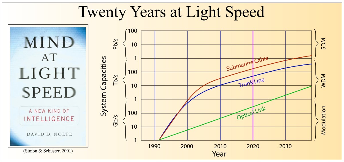
At the 20-year anniversary of the publication of my book Mind at Light Speed (Free Press, 2001), this blog is the third in a series reviewing progress in three generations of Machines of Light over the past 20 years (see my previous blogs on the future of the photonic internet and on all-optical computers). This third and final update reviews progress on the third generation of the Machines of Light: the Quantum Optical Generation. Of the three generations, this is the one that is changing the fastest.

Quantum computing is almost here … and it will be at room temperature, using light, in photonic integrated circuits!

Quantum Computing with Linear Optics

Twenty years ago in 2001, Emanuel Knill and Raymond LaFlamme at Los Alamos National Lab, with Gerald Mulburn at the University of Queensland, Australia, published a revolutionary theoretical paper (known as KLM) in Nature on quantum computing with linear optics: “A scheme for efficient quantum computation with linear optics” [1]. Up until that time, it was believed that a quantum computer — if it was going to have the property of a universal Turing machine — needed to have at least some nonlinear interactions among qubits in a quantum gate. For instance, an example of a two-qubit gate is a controlled-NOT, or CNOT, gate shown in Fig. 1 with the Truth Table and the equivalent unitary matrix. It clear that one qubit is controlling the other, telling it what to do.

The quantum CNOT gate gets interesting when the control line has a quantum superposition, then the two outputs become entangled.

Entanglement is a strange process that is unique to quantum systems and has no classical analog. It also has no simple intuitive explanation. By any normal logic, if the control line passes through the gate unaltered, then absolutely nothing interesting should be happening on the Control-Out line. But that’s not the case. The control line going in was a separate state. If some measurement were made on it, either a 1 or 0 would be seen with equal probability. But coming out of the CNOT, the signal has somehow become perfectly correlated with whatever value is on the Signal-Out line. If the Signal-Out is measured, the measurement process collapses the state of the Control-Out to a value equal to the measured signal. The outcome of the control line becomes 100% certain even though nothing was ever done to it! This entanglement generation is one reason the CNOT is often the gate of choice when constructing quantum circuits to perform interesting quantum algorithms.

However, optical implementation of a CNOT is a problem, because light beams and photons really do not like to interact with each other. This is the problem with all-optical classical computers too (see my previous blog). There are ways of getting light to interact with light, for instance inside nonlinear optical materials. And in the case of quantum optics, a single atom in an optical cavity can interact with single photons in ways that can act like a CNOT or related gates. But the efficiencies are very low and the costs to implement it are very high, making it difficult or impossible to scale such systems up into whole networks needed to make a universal quantum computer.

Therefore, when KLM published their idea for quantum computing with linear optics, it caused a shift in the way people were thinking about optical quantum computing. A universal optical quantum computer could be built using just light sources, beam splitters and photon detectors.

The way that KLM gets around the need for a direct nonlinear interaction between two photons is to use postselection. They run a set of photons — signal photons and ancilla (test) photons — through their linear optical system and they detect (i.e., theoretically…the paper is purely a theoretical proposal) the ancilla photons. If these photons are not detected where they are wanted, then that iteration of the computation is thrown out, and it is tried again and again, until the photons end up where they need to be. When the ancilla outcomes are finally what they need to be, this run is selected because the signal state are known to have undergone a known transformation. The signal photons are still unmeasured at this point and are therefore in quantum superpositions that are useful for quantum computation. Postselection uses entanglement and measurement collapse to put the signal photons into desired quantum states. Postselection provides an effective nonlinearity that is induced by the wavefunction collapse of the entangled state. Of course, the down side of this approach is that many iterations are thrown out — the computation becomes non-deterministic.

KLM could get around most of the non-determinism by using more and more ancilla photons, but this has the cost of blowing up the size and cost of the implementation, so their scheme was not imminently practical. But the important point was that it introduced the idea of linear quantum computing. (For this, Milburn and his collaborators have my vote for a future Nobel Prize.) Once that idea was out, others refined it, and improved upon it, and found clever ways to make it more efficient and more scalable. Many of these ideas relied on a technology that was co-evolving with quantum computing — photonic integrated circuits (PICs).

Quantum Photonic Integrated Circuits (QPICs)

Never underestimate the power of silicon. The amount of time and energy and resources that have now been invested in silicon device fabrication is so astronomical that almost nothing in this world can displace it as the dominant technology of the present day and the future. Therefore, when a photon can do something better than an electron, you can guess that eventually that photon will be encased in a silicon chip–on a photonic integrated circuit (PIC).

The dream of integrated optics (the optical analog of integrated electronics) has been around for decades, where waveguides take the place of conducting wires, and interferometers take the place of transistors — all miniaturized and fabricated in the thousands on silicon wafers. The advantages of PICs are obvious, but it has taken a long time to develop. When I was a post-doc at Bell Labs in the late 1980’s, everyone was talking about PICs, but they had terrible fabrication challenges and terrible attenuation losses. Fortunately, these are just technical problems, not limited by any fundamental laws of physics, so time (and an army of researchers) has chipped away at them.

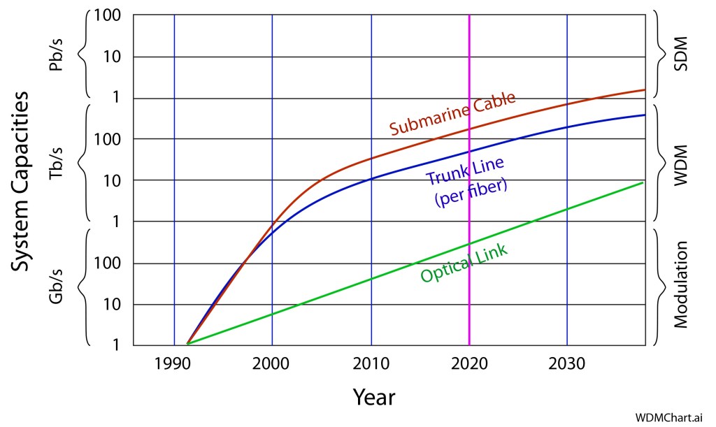
One of the driving forces behind the maturation of PIC technology is photonic fiber optic communications (as discussed in a previous blog). Photons are clear winners when it comes to long-distance communications. In that sense, photonic information technology is a close cousin to silicon — photons are no less likely to be replaced by a future technology than silicon is. Therefore, it made sense to bring the photons onto the silicon chips, tapping into the full array of silicon fab resources so that there could be seamless integration between fiber optics doing the communications and the photonic chips directing the information. Admittedly, photonic chips are not yet all-optical. They still use electronics to control the optical devices on the chip, but this niche for photonics has provided a driving force for advancements in PIC fabrication.

Fig. 2 Schematic of a silicon photonic integrated circuit (PIC). The waveguides can be silica or nitride deposited on the silicon chip. From the Comsol WebSite.

One side-effect of improved PIC fabrication is low light losses. In telecommunications, this loss is not so critical because the systems use OEO regeneration. But less loss is always good, and the PICs can now safeguard almost every photon that comes on chip — exactly what is needed for a quantum PIC. In a quantum photonic circuit, every photon is valuable and informative and needs to be protected. The new PIC fabrication can do this. In addition, light switches for telecom applications are built from integrated interferometers on the chip. It turns out that interferometers at the single-photon level are unitary quantum gates that can be used to build universal photonic quantum computers. So the same technology and control that was used for telecom is just what is needed for photonic quantum computers. In addition, integrated optical cavities on the PICs, which look just like wavelength filters when used for classical optics, are perfect for producing quantum states of light known as squeezed light that turn out to be valuable for certain specialty types of quantum computing.

Therefore, as the concepts of linear optical quantum computing advanced through that last 20 years, the hardware to implement those concepts also advanced, driven by a highly lucrative market segment that provided the resources to tap into the vast miniaturization capabilities of silicon chip fabrication. Very fortuitous!

Room-Temperature Quantum Computers

There are many radically different ways to make a quantum computer. Some are built of superconducting circuits, others are made from semiconductors, or arrays of trapped ions, or nuclear spins on nuclei on atoms in molecules, and of course with photons. Up until about 5 years ago, optical quantum computers seemed like long shots. Perhaps the most advanced technology was the superconducting approach. Superconducting quantum interference devices (SQUIDS) have exquisite sensitivity that makes them robust quantum information devices. But the drawback is the cold temperatures that are needed for them to work. Many of the other approaches likewise need cold temperature–sometimes astronomically cold temperatures that are only a few thousandths of a degree above absolute zero Kelvin.

Cold temperatures and quantum computing seemed a foregone conclusion — you weren’t ever going to separate them — and for good reason. The single greatest threat to quantum information is decoherence — the draining away of the kind of quantum coherence that allows interferences and quantum algorithms to work. In this way, entanglement is a two-edged sword. On the one hand, entanglement provides one of the essential resources for the exponential speed-up of quantum algorithms. But on the other hand, if a qubit “sees” any environmental disturbance, then it becomes entangled with that environment. The entangling of quantum information with the environment causes the coherence to drain away — hence decoherence. Hot environments disturb quantum systems much more than cold environments, so there is a premium for cooling the environment of quantum computers to as low a temperature as they can. Even so, decoherence times can be microseconds to milliseconds under even the best conditions — quantum information dissipates almost as fast as you can make it.

Enter the photon! The bottom line is that photons don’t interact. They are blind to their environment. This is what makes them perfect information carriers down fiber optics. It is also what makes them such good qubits for carrying quantum information. You can prepare a photon in a quantum superposition just by sending it through a lossless polarizing crystal, and then the superposition will last for as long as you can let the photon travel (at the speed of light). Sometimes this means putting the photon into a coil of fiber many kilometers long to store it, but that is OK — a kilometer of coiled fiber in the lab is no bigger than a few tens of centimeters. So the same properties that make photons excellent at carrying information also gives them very small decoherence. And after the KLM schemes began to be developed, the non-interacting properties of photons were no longer a handicap.

In the past 5 years there has been an explosion, as well as an implosion, of quantum photonic computing advances. The implosion is the level of integration which puts more and more optical elements into smaller and smaller footprints on silicon PICs. The explosion is the number of first-of-a-kind demonstrations: the first universal optical quantum computer [2], the first programmable photonic quantum computer [3], and the first (true) quantum computational advantage [4].

All of these “firsts” operate at room temperature. (There is a slight caveat: The photon-number detectors are actually superconducting wire detectors that do need to be cooled. But these can be housed off-chip and off-rack in a separate cooled system that is coupled to the quantum computer by — no surprise — fiber optics.) These are the advantages of photonic quantum computers: hundreds of qubits integrated onto chips, room-temperature operation, long decoherence times, compatibility with telecom light sources and PICs, compatibility with silicon chip fabrication, universal gates using postselection, and more. Despite the head start of some of the other quantum computing systems, photonics looks like it will be overtaking the others within only a few years to become the dominant technology for the future of quantum computing. And part of that future is being helped along by a new kind of quantum algorithm that is perfectly suited to optics.

Fig. 3 Superconducting photon counting detector. From WebSite

A New Kind of Quantum Algorithm: Boson Sampling

In 2011, Scott Aaronson (then at at MIT) published a landmark paper titled “The Computational Complexity of Linear Optics” with his post-doc, Anton Arkhipov [5].  The authors speculated on whether there could be an application of linear optics, not requiring the costly step of post-selection, that was still useful for applications, while simultaneously demonstrating quantum computational advantage.  In other words, could one find a linear optical system working with photons that could solve problems intractable to a classical computer?  To their own amazement, they did!  The answer was something they called “boson sampling”.

To get an idea of what boson sampling is, and why it is very hard to do on a classical computer, think of the classic demonstration of the normal probability distribution found at almost every science museum you visit, illustrated in Fig. 2.  A large number of ping-pong balls are dropped one at a time through a forest of regularly-spaced posts, bouncing randomly this way and that until they are collected into bins at the bottom.  Bins near the center collect many balls, while bins farther to the side have fewer.  If there are many balls, then the stacked heights of the balls in the bins map out a Gaussian probability distribution.  The path of a single ping-pong ball represents a series of “decisions” as it hits each post and goes left or right, and the number of permutations of all the possible decisions among all the other ping-pong balls grows exponentially—a hard problem to tackle on a classical computer.

Fig. 4 Ping-pont ball normal distribution. Watch the YouTube video.


In the paper, Aaronson considered a quantum analog to the ping-pong problem in which the ping-pong balls are replaced by photons, and the posts are replaced by beam splitters.  As its simplest possible implementation, it could have two photon channels incident on a single beam splitter.  The well-known result in this case is the “HOM dip” [6] which is a consequence of the boson statistics of the photon.  Now scale this system up to many channels and a cascade of beam splitters, and one has an N-channel multi-photon HOM cascade.  The output of this photonic “circuit” is a sampling of the vast number of permutations allowed by bose statistics—boson sampling. 

To make the problem more interesting, Aaronson allowed the photons to be launched from any channel at the top (as opposed to dropping all the ping-pong balls at the same spot), and they allowed each beam splitter to have adjustable phases (photons and phases are the key elements of an interferometer).  By adjusting the locations of the photon channels and the phases of the beam splitters, it would be possible to “program” this boson cascade to mimic interesting quantum systems or even to solve specific problems, although they were not thinking that far ahead.  The main point of the paper was the proposal that implementing boson sampling in a photonic circuit used resources that scaled linearly in the number of photon channels, while the problems that could be solved grew exponentially—a clear quantum computational advantage [4]. 

On the other hand, it turned out that boson sampling is not universal—one cannot construct a universal quantum computer out of boson sampling.  The first proposal was a specialty algorithm whose main function was to demonstrate quantum computational advantage rather than do something specifically useful—just like Deutsch’s first algorithm.  But just like Deutsch’s algorithm, which led ultimately to Shor’s very useful prime factoring algorithm, boson sampling turned out to be the start of a new wave of quantum applications.

Shortly after the publication of Aaronson’s and Arkhipov’s paper in 2011, there was a flurry of experimental papers demonstrating boson sampling in the laboratory [7, 8].  And it was discovered that boson sampling could solve important and useful problems, such as the energy levels of quantum systems, and network similarity, as well as quantum random-walk problems. Therefore, even though boson sampling is not strictly universal, it solves a broad class of problems. It can be viewed more like a specialty chip than a universal computer, like the now-ubiquitous GPU’s are specialty chips in virtually every desktop and laptop computer today. And the room-temperature operation significantly reduces cost, so you don’t need a whole government agency to afford one. Just like CPU costs followed Moore’s Law to the point where a Raspberry Pi computer costs $40 today, the photonic chips may get onto their own Moore’s Law that will reduce costs over the next several decades until they are common (but still specialty and probably not cheap) computers in academia and industry. A first step along that path was a recently-demonstrated general programmable room-temperature photonic quantum computer.

Fig. 5 A classical Galton board on the left, and a photon-based boson sampling on the right. From the Walmsley (Oxford) WebSite.

A Programmable Photonic Quantum Computer: Xanadu’s X8 Chip

I don’t usually talk about specific companies, but the new photonic quantum computer chip from Xanadu, based in Toronto, Canada, feels to me like the start of something big. In the March 4, 2021 issue of Nature magazine, researchers at the company published the experimental results of their X8 photonic chip [3]. The chip uses boson sampling of strongly non-classical light. This was the first generally programmable photonic quantum computing chip, programmed using a quantum programming language they developed called Strawberry Fields. By simply changing the quantum code (using a simple conventional computer interface), they switched the computer output among three different quantum applications: transitions among states (spectra of molecular states), quantum docking, and similarity between graphs that represent two different molecules. These are radically different physics and math problems, yet the single chip can be programmed on the fly to solve each one.

The chip is constructed of nitride waveguides on silicon, shown in Fig. 6. The input lasers drive ring oscillators that produce squeezed states through four-wave mixing. The key to the reprogrammability of the chip is the set of phase modulators that use simple thermal changes on the waveguides. These phase modulators are changed in response to commands from the software to reconfigure the application. Although they switch slowly, once they are set to their new configuration, the computations take place “at the speed of light”. The photonic chip is at room temperature, but the outputs of the four channels are sent by fiber optic to a cooled unit containing the superconductor nanowire photon counters.

Fig. 6 The Xanadu X8 photonic quantum computing chip. From Ref.
Fig. 7 To see the chip in operation, see the YouTube video.

Admittedly, the four channels of the X8 chip are not large enough to solve the kinds of problems that would require a quantum computer, but the company has plans to scale the chip up to 100 channels. One of the challenges is to reduce the amount of photon loss in a multiplexed chip, but standard silicon fabrication approaches are expected to reduce loss in the next generation chips by an order of magnitude.

Additional companies are also in the process of entering the photonic quantum computing business, such as PsiQuantum, which recently closed a $450M funding round to produce photonic quantum chips with a million qubits. The company is led by Jeremy O’Brien from Bristol University who has been a leader in photonic quantum computing for over a decade.

Stay tuned!

By David D. Nolte, Dec. 20, 2021

Further Reading

• David D. Nolte, “Interference: A History of Interferometry and the Scientists who Tamed Light” (Oxford University Press, to be published in 2023)

• J. L. O’Brien, A. Furusawa, and J. Vuckovic, “Photonic quantum technologies,” Nature Photonics, Review vol. 3, no. 12, pp. 687-695, Dec (2009)

• T. C. Ralph and G. J. Pryde, “Optical Quantum Computation,” in Progress in Optics, Vol 54, vol. 54, E. Wolf Ed.,  (2010), pp. 209-269.

• S. Barz, “Quantum computing with photons: introduction to the circuit model, the one-way quantum computer, and the fundamental principles of photonic experiments,” (in English), Journal of Physics B-Atomic Molecular and Optical Physics, Article vol. 48, no. 8, p. 25, Apr (2015), Art no. 083001

References

[1] E. Knill, R. Laflamme, and G. J. Milburn, “A scheme for efficient quantum computation with linear optics,” Nature, vol. 409, no. 6816, pp. 46-52, Jan (2001)

[2] J. Carolan, J. L. O’Brien et al, “Universal linear optics,” Science, vol. 349, no. 6249, pp. 711-716, Aug (2015)

[3] J. M. Arrazola, et al, “Quantum circuits with many photons on a programmable nanophotonic chip,” Nature, vol. 591, no. 7848, pp. 54-+, Mar (2021)

[4] H.-S. Zhong J.-W. Pan et al, “Quantum computational advantage using photons,” Science, vol. 370, no. 6523, p. 1460, (2020)

[5] S. Aaronson and A. Arkhipov, “The Computational Complexity of Linear Optics,” in 43rd ACM Symposium on Theory of Computing, San Jose, CA, Jun 06-08 2011, NEW YORK: Assoc Computing Machinery, in Annual ACM Symposium on Theory of Computing, 2011, pp. 333-342

[6] C. K. Hong, Z. Y. Ou, and L. Mandel, “Measurement of subpicosecond time intervals between 2 photons by interference,” Physical Review Letters, vol. 59, no. 18, pp. 2044-2046, Nov (1987)

[7] J. B. Spring, I. A. Walmsley et al, “Boson Sampling on a Photonic Chip,” Science, vol. 339, no. 6121, pp. 798-801, Feb (2013)

[8] M. A. Broome, A. Fedrizzi, S. Rahimi-Keshari, J. Dove, S. Aaronson, T. C. Ralph, and A. G. White, “Photonic Boson Sampling in a Tunable Circuit,” Science, vol. 339, no. 6121, pp. 794-798, Feb (2013)


New from Oxford Press: The History of Optical Interferometry (Late Summer 2023)

Twenty Years at Light Speed: Fiber Optics and the Future of the Photonic Internet

Twenty years ago this November, my book Mind at Light Speed: A New Kind of Intelligence was published by The Free Press (Simon & Schuster, 2001).  The book described the state of optical science at the turn of the Millennium through three generations of Machines of Light:  The Optoelectronic Generation of electronic control meshed with photonic communication; The All-Optical Generation of optical logic; and The Quantum Optical Generation of quantum communication and computing.

To mark the occasion of the publication, this Blog Post begins a three-part series that updates the state-of-the-art of optical technology, looking at the advances in optical science and technology over the past 20 years since the publication of Mind at Light Speed.  This first blog reviews fiber optics and the photonic internet.  The second blog reviews all-optical communication and computing.  The third and final blog reviews the current state of photonic quantum communication and computing.

The Wabash Yacht Club

During late 1999 and early 2000, while I was writing Mind at Light Speed, my wife Laura and I would often have lunch at the ironically-named Wabash Yacht Club.  Not only was it not a Yacht Club, but it was a dark and dingy college-town bar located in a drab 70-‘s era plaza in West Lafayette, Indiana, far from any navigable body of water.  But it had a great garlic burger and we loved the atmosphere.

The Wabash River. No yachts. (https://www.riverlorian.com/wabash-river)

One of the TV monitors in the bar was always tuned to a station that covered stock news, and almost every day we would watch the NASDAQ rise 100 points just over lunch.  This was the time of the great dot-com stock-market bubble—one of the greatest speculative bubbles in the history of world economics.  In the second quarter of 2000, total US venture capital investments exceeded $30B as everyone chased the revolution in consumer market economics.

Fiber optics will remain the core technology of the internet for the foreseeable future.

Part of that dot-com bubble was a massive bubble in optical technology companies, because everyone knew that the dot-com era would ride on the back of fiber optics telecommunications.  Fiber optics at that time had already revolutionized transatlantic telecommunications, and there seemed to be no obstacle for it to do the same land-side with fiber optics to every home bringing every dot-com product to every house and every movie ever made.  What would make this possible was the tremendous information bandwidth that can be crammed into tiny glass fibers in the form of photon packets traveling at the speed of light.

Doing optics research at that time was a heady experience.  My research on real-time optical holography was only on the fringe of optical communications, but at the CLEO conference on lasers and electro-optics, I was invited by tiny optics companies to giant parties, like a fully-catered sunset cruise on a schooner sailing Baltimore’s inner harbor.  Venture capital scouts took me to dinner in San Francisco with an eye to scoop up whatever patents I could dream of.  And this was just the side show.  At the flagship fiber-optics conference, the Optical Fiber Conference (OFC) of the OSA, things were even crazier.  One tiny company that made a simple optical switch went almost overnight from a company worth a couple of million to being bought out by Nortel (the giant Canadian telecommunications conglomerate of the day) for over 4 billion dollars.

The Telecom Bubble and Bust

On the other side from the small mom-and-pop optics companies were the giants like Corning (who made the glass for the glass fiber optics) and Nortel.  At the height of the telecom bubble in September 2000, Nortel had a capitalization of almost $400B Canadian dollars due to massive speculation about the markets around fiber-optic networks.

One of the central questions of the optics bubble of Y2K was what the new internet market would look like.  Back then, fiber was only beginning to connect to distribution nodes that were connected off the main cross-country trunk lines.  Cable TV dominated the market with fixed programming where you had to watch whatever they transmitted whenever they transmitted it.  Google was only 2 years old, and Youtube didn’t even exist then—it was founded in 2005.  Everyone still shopped at malls, while Amazon had only gone public three years before.

There were fortune tellers who predicted that fiber-to-the-home would tap a vast market of online commerce where you could buy anything you wanted and have it delivered to your door.  They foretold of movies-on-demand, where anyone could stream any movie they wanted at any time.  They also foretold of phone calls and video chats that never went over the phone lines ruled by the telephone monopolies.  The bandwidth, the data rates, that these markets would drive were astronomical.  The only technology at that time that could support such high data rates was fiber optics.

At first, these fortune tellers drove an irrational exuberance.  But as the stocks inflated, there were doomsayers who pointed out that the costs at that time of bringing fiber into homes was prohibitive. And the idea that people would be willing to pay for movies-on-demand was laughable.  The cost of the equipment and the installation just didn’t match what then seemed to be a sparse market demand.  Furthermore, the fiber technology in the year 2000 couldn’t even get to the kind of data rates that could support these dreams.

In March of 2000 the NASDAQ hit a high of 5000, and then the bottom fell out.

By November 2001 the NASDAQ had fallen to 1500.  One of the worst cases of the telecom bust was Nortel whose capitalization plummeted from $400B at its high to $5B Canadian by August 2002.  Other optics companies fared little better.

The main questions, as we stand now looking back from 20 years in the future, are: What in real life motivated the optics bubble of 2000?  And how far has optical technology come since then?  The surprising answer is that the promise of optics in 2000 was not wrong—the time scale was just off. 

Fiber to the Home

Today, fixed last-mile broadband service is an assumed part of life in metro areas in the US.  This broadband takes on three forms: legacy coaxial cable, 4G wireless soon to be upgraded to 5G, and fiber optics.  There are arguments pro and con for each of these technologies, especially moving forward 10 or 20 years or more, and a lot is at stake.  The global market revenue was $108 Billion in 2020 and is expected to reach $200 Billion in 2027, growing at over 9% from 2021 to 2027.

(ShutterStock_75369058.jpg)

To sort through the pros and cons to pick the wining technology, several key performance parameters must be understood for each technology.  The two most important performance measures are bandwidth and latency.  Bandwidth is the data rate—how many bits per second can you get to the home.  Latency is a little more subtle.  It is the time it takes to complete a transmission.  This time includes the actual time for information to travel from a transmitter to a receiver, but that is rarely the major contributor.  Currently, almost all of the latency is caused by the logical operations needed to move the information onto and off of the home data links. 

Coax (short for coaxial cable) is attractive because so much of the last-mile legacy hardware is based on the old cable services.  But coax cable has very limited bandwidth and high latency. As a broadband technology, it is slowly disappearing.

Wireless is attractive because the information is transmitted in the open air without any need for physical wires or fibers.  But high data rates require high frequency.  For instance, 4G wireless operates at frequencies between 700 MHz to 2.6 GHz.  Current WiFi is 2.4 GHz or 5 GHz, and next-generation 5G will have 26 GHz using millimeter wave technology, and WiGig is even more extreme at 60 GHz.  While WiGig will deliver up to 10 Gbits per second, as everyone with wireless routers in their homes knows, the higher the frequency, the more it is blocked by walls or other obstacles.  Even 5 GHz is mostly attenuated by walls, and the attenuation gets worse as the frequency gets higher.  Testing of 5G networks has shown that cell towers need to be closely spaced to allow seamless coverage.  And the crazy high frequency of WiGig all but guarantees that it will only be usable for line-of-sight communication within a home or in an enterprise setting. 

Fiber for the last mile, on the other hand, has multiple advantages.  Chief among these is that fiber is passive.  It is a light pipe that has ten thousand times more usable bandwidth than a coaxial cable.  For instance, lab tests have pushed up to 100 Tbit/sec over kilometers of fiber.  To access that bandwidth, the input and output hardware can be continually upgraded, while the installed fiber is there to handle pretty much any amount of increasing data rates for the next 10 or 20 years.  Fiber installed today is supporting 1 Gbit/sec data rates, and the existing protocol will work up to 10 Gbit/sec—data rates that can only be hoped for with WiFi.  Furthermore, optical communications on fiber have latencies of around 1.5 msec over 20 kilometers compared with 4G LTE that has a latency of 8 msec over 1 mile.  The much lower latency is key to support activities that cannot stand much delay, such as voice over IP, video chat, remote controlled robots, and virtual reality (i.e., gaming).  On top of all of that, the internet technology up to the last mile is already almost all optical.  So fiber just extends the current architecture across the last mile.

Therefore, fixed fiber last-mile broadband service is a technology winner.  Though the costs can be higher than for WiFi or coax in the short run for installation, the long-run costs are lower when amortized over the lifetime of the installed fiber which can exceed 25 years.

It is becoming routine to have fiber-to-the-curb (FTTC) where a connection box converts photons in fibers into electrons on copper to take the information into the home.  But a market also exists in urban settings for fiber-to-the-home (FTTH) where the fiber goes directly into the house to a receiver and only then would the information be converted from photons to electrons and electronics.

Shortly after Mind at Light Speed was published in 2001, I was called up by a reporter for the Seattle Times who wanted to know my thoughts about FTTH.  When I extolled its virtue, he nearly hung up on me.  He was in the middle of debunking the telecom bubble and his premise was that FTTH was a fraud.  In 2001 he might have been right.  But in 2021, FTTH is here, it is expanding, and it will continue to do so for at least another quarter century.  Fiber to the home will become the legacy that some future disruptive technology will need to displace.

Fig. 1 Optical data rates on optical links, trunk lines and submarine cables over the past 30 years and projecting into the future. Redrawn from Refs. [1, 2]

Trunk-Line Fiber Optics

Despite the rosy picture for Fiber to the Home, a storm is brewing for the optical trunk lines.  The total traffic on the internet topped a billion Terrabytes in 2019 and is growing fast, doubling about every 2 years on an exponential growth curve.  In 20 years, that becomes another factor of a thousand more traffic in 2040 than today.  Therefore, the technology companies that manage and supply the internet worry about a capacity crunch that is fast approaching when there will be more demand than the internet can supply.

Over the past 20 years, the data rates on the fiber trunk lines—the major communication links that span the United States—matched demand by packing more bits in more ways into the fibers.  Up to 2009, increased data rates were achieved using dispersion-managed wavelength-division multiplexing (WDM) which means that they kept adding more lasers of slightly different colors to send the optical bits down the fiber.  For instance, in 2009 the commercial standard was 80 colors each running at 40 Gbit/sec for a total of 3.2 Tbit/sec down a single fiber. 

Since 2009, increased bandwidth has been achieved through coherent WDM, where not only the amplitude of light but also the phase of the light is used to encode bits of information using interferometry.  We are still in the coherent WDM era as improved signal processing is helping to fill the potential coherent bandwidth of a fiber.  Commercial protocols using phase-shift keying, quadrature phase-shift keying, and 16-quadrature amplitude modulation currently support 50 Gbit/sec, 100 Gbit/sec and 200 Gbit/sec, respectively.  But the capacity remaining is shrinking, and several years from now, a new era will need to begin in order to keep up with demand.  But if fibers are already using time, color, polarization and phase to carry information, what is left? 

The answer is space!

Coming soon will be commercial fiber trunk lines that use space-division multiplexing (SDM).  The simplest form is already happening now as fiber bundles are replacing single-mode fibers.  If you double the number of fibers in a cable, then you double the data rate of the cable.  But the problem with this simple approach is the scaling.  If you double just 10 times, then you need 1024 fibers in a single cable—each fiber needing its own hardware to launch the data and retrieve it at the other end.  This is linear scaling, which is bad scaling for commercial endeavors. 

Fig. 2 Fiber structures for space-division multiplexing (SDM). Fiber bundles are cables of individual single-mode fibers. Multi-element fibers (MEF) are single-mode fibers formed together inside the coating. Multi-core fibers (MCF) have multiple cores within the cladding. Few-mode fibers (FMF) are multi-mode fibers with small mode numbers. Coupled core (CC) fibers are multi-core fibers in which the cores are close enough that the light waves are coupled into coupled spatial modes. Redrawn from Ref. [3]

Therefore, alternatives for tapping into SDM are being explored in lab demonstrations now that have sublinear scaling (costs don’t rise as fast as improved capacity).  These include multi-element fibers where multiple fiber optical elements are manufactured as a group rather than individually and then combined into a cable.  There are also multi-core fibers, where multiple fibers share the same cladding.  These approaches provide multiple fibers for multiple channels without a proportional rise in cost.

More exciting are approaches that use few-mode-fibers (FMF) to support multiple spatial modes traveling simultaneously down the same fiber.  In the same vein are coupled-core fibers which is a middle ground between multi-core fibers and few-mode fibers in that individual cores can interact within the cladding to support coupled spatial modes that can encode separate spatial channels.  Finally, combinations of approaches can use multiple formats.  For instance, a recent experiment combined FMF and MCF that used 19 cores each supporting 6 spatial modes for a total of 114 spatial channels.

However, space-division multiplexing has been under development for several years now, yet it has not fully moved into commercial systems. This may be a sign that the doubling rate of bandwidth may be starting to slow down, just as Moore’s Law slowed down for electronic chips.  But there were doomsayers foretelling the end of Moore’s Law for decades before it actually slowed down, because new ideas cannot be predicted. But even if the full capacity of fiber is being approached, there is certainly nothing that will replace fiber with any better bandwidth.  So fiber optics will remain the core technology of the internet for the foreseeable future. 

But what of the other generations of Machines of Light: the all-optical and the quantum-optical generations?  How have optics and photonics fared in those fields?  Stay tuned for my next blogs to find out.

By David D. Nolte, Nov. 8, 2021

Bibliography

[1] P. J. Winzer, D. T. Neilson, and A. R. Chraplyvy, “Fiber-optic transmission and networking: the previous 20 and the next 20 years,” Optics Express, vol. 26, no. 18, pp. 24190-24239, Sep (2018) [Link]

[2] W. Shi, Y. Tian, and A. Gervais, “Scaling capacity of fiber-optic transmission systems via silicon photonics,” Nanophotonics, vol. 9, no. 16, pp. 4629-4663, Nov (2020)

[3] E. Agrell, M. Karlsson, A. R. Chraplyvy, D. J. Richardson, P. M. Krummrich, P. Winzer, K. Roberts, J. K. Fischer, S. J. Savory, B. J. Eggleton, M. Secondini, F. R. Kschischang, A. Lord, J. Prat, I. Tomkos, J. E. Bowers, S. Srinivasan, M. Brandt-Pearce, and N. Gisin, “Roadmap of optical communications,” Journal of Optics, vol. 18, no. 6, p. 063002, 2016/05/04 (2016) [Link]

A Short History of the Photon

The quantum of light—the photon—is a little over 100 years old.  It was born in 1905 when Einstein merged Planck’s blackbody quantum hypothesis with statistical mechanics and concluded that light itself must be quantized.  No one believed him!  Fast forward to today, and the photon is a modern workhorse of modern quantum technology.  Quantum encryption and communication are performed almost exclusively with photons, and many prototype quantum computers are optics based.  Quantum optics also underpins atomic and molecular optics (AMO), which is one of the hottest and most rapidly advancing  frontiers of physics today.

Only after the availability of “quantum” light sources … could photon numbers be manipulated at will, launching the modern era of quantum optics.

This blog tells the story of the early days of the photon and of quantum optics.  It begins with Einstein in 1905 and ends with the demonstration of photon anti-bunching that was the first fundamentally quantum optical phenomenon observed seventy years later in 1977.  Across that stretch of time, the photon went from a nascent idea in Einstein’s fertile brain to the most thoroughly investigated quantum particle in the realm of physics.

The Photon: Albert Einstein (1905)

When Planck presented his quantum hypothesis in 1900 to the German Physical Society [1], his model of black body radiation retained all its classical properties but one—the quantized interaction of light with matter.  He did not think yet in terms of quanta, only in terms of steps in a continuous interaction.

The quantum break came from Einstein when he published his 1905 paper proposing the existence of the photon—an actual quantum of light that carried with it energy and momentum [2].  His reasoning was simple and iron-clad, resting on Planck’s own blackbody relation that Einstein combined with simple reasoning from statistical mechanics.  He was led inexorably to the existence of the photon.  Unfortunately, almost no one believed him (see my blog on Einstein and Planck). 

This was before wave-particle duality in quantum thinking, so the notion that light—so clearly a wave phenomenon—could be a particle was unthinkable.  It had taken half of the 19th century to rid physics of Newton’s corpuscules and emmisionist theories of light, so to bring it back at the beginning of the 20th century seemed like a great blunder.  However, Einstein persisted.

In 1909 he published a paper on the fluctuation properties of light [3] in which he proposed that the fluctuations observed in light intensity had two contributions: one from the discreteness of the photons (what we call “shot noise” today) and one from the fluctuations in the wave properties.  Einstein was proposing that both particle and wave properties contributed to intensity fluctuations, exhibiting simultaneous particle-like and wave-like properties.  This was one of the first expressions of wave-particle duality in modern physics.

In 1916 and 1917 Einstein took another bold step and proposed the existence of stimulated emission [4].  Once again, his arguments were based on simple physics—this time the principle of detailed balance—and he was led to the audacious conclusion that one photon can stimulated the emission of another.  This would become the basis of the laser forty-five years later.

While Einstein was confident in the reality of the photon, others sincerely doubted its existence.  Robert Milliken (1868 – 1953) decided to put Einstein’s theory of photoelectron emission to the most stringent test ever performed.  In 1915 he painstakingly acquired the definitive dataset with the goal to refute Einstein’s hypothesis, only to confirm it in spectacular fashion [5].  Partly based on Milliken’s confirmation of Einstein’s theory of the photon, Einstein was awarded the Nobel Prize in Physics in 1921.

Einstein at a blackboard.

From that point onward, the physical existence of the photon was accepted and was incorporated routinely into other physical theories.  Compton used the energy and the momentum of the photon in 1922 to predict and measure Compton scattering of x-rays off of electrons [6].  The photon was given its modern name by Gilbert Lewis in 1926 [7].

Single-Photon Interference: Geoffry Taylor (1909)

If a light beam is made up of a group of individual light quanta, then in the limit of very dim light, there should just be one photon passing through an optical system at a time.  Therefore, to do optical experiments on single photons, one just needs to reach the ultimate dim limit.  As simple and clear as this argument sounds, it has problems that only were sorted out after the Hanbury Brown and Twiss experiments in the 1950’s and the controversy they launched (see below).  However, in 1909, this thinking seemed like a clear approach for looking for deviations in optical processes in the single-photon limit.

In 1909, Geoffry Ingram Taylor (1886 – 1975) was an undergraduate student at Cambridge University and performed a low-intensity Young’s double-slit experiment (encouraged by J. J. Thomson).  At that time the idea of Einstein’s photon was only 4 years old, and Bohr’s theory of the hydrogen atom was still a year away.  But Thomson believed that if photons were real, then their existence could possibly show up as deviations in experiments involving single photons.  Young’s double-slit experiment is the classic demonstration of the classical wave nature of light, so performing it under conditions when (on average) only a single photon was in transit between a light source and a photographic plate seemed like the best place to look.

G. I. Taylor

The experiment was performed by finding an optimum exposure of photographic plates in a double slit experiment, then reducing the flux while increasing the exposure time, until the single-photon limit was achieved while retaining the same net exposure of the photographic plate.  Under the lowest intensity, when only a single photon was in transit at a time (on average), Taylor performed the exposure for three months.  To his disappointment, when he developed the film, there was no significant difference between high intensity and low intensity interference fringes [8].  If photons existed, then their quantized nature was not showing up in the low-intensity interference experiment.

The reason that there is no single-photon-limit deviation in the behavior of the Young double-slit experiment is because Young’s experiment only measures first-order coherence properties.  The average over many single-photon detection events is described equally well either by classical waves or by quantum mechanics.  Quantized effects in the Young experiment could only appear in fluctuations in the arrivals of photons, but in Taylor’s day there was no way to detect the arrival of single photons. 

Quantum Theory of Radiation : Paul Dirac (1927)

After Paul Dirac (1902 – 1984) was awarded his doctorate from Cambridge in 1926, he received a stipend that sent him to work with Niels Bohr (1885 – 1962) in Copenhagen. His attention focused on the electromagnetic field and how it interacted with the quantized states of atoms.  Although the electromagnetic field was the classical field of light, it was also the quantum field of Einstein’s photon, and he wondered how the quantized harmonic oscillators of the electromagnetic field could be generated by quantum wavefunctions acting as operators.  He decided that, to generate a photon, the wavefunction must operate on a state that had no photons—the ground state of the electromagnetic field known as the vacuum state.

Dirac put these thoughts into their appropriate mathematical form and began work on two manuscripts.  The first manuscript contained the theoretical details of the non-commuting electromagnetic field operators.  He called the process of generating photons out of the vacuum “second quantization”.  In second quantization, the classical field of electromagnetism is converted to an operator that generates quanta of the associated quantum field out of the vacuum (and also annihilates photons back into the vacuum).  The creation operators can be applied again and again to build up an N-photon state containing N photons that obey Bose-Einstein statistics, as they must, as required by their integer spin, and agreeing with Planck’s blackbody radiation. 

Dirac then showed how an interaction of the quantized electromagnetic field with quantized energy levels involved the annihilation and creation of photons as they promoted electrons to higher atomic energy levels, or demoted them through stimulated emission.  Very significantly, Dirac’s new theory explained the spontaneous emission of light from an excited electron level as a direct physical process that creates a photon carrying away the energy as the electron falls to a lower energy level.  Spontaneous emission had been explained first by Einstein more than ten years earlier when he derived the famous A and B coefficients [4], but the physical mechanism for these processes was inferred rather than derived. Dirac, in late 1926, had produced the first direct theory of photon exchange with matter [9]

Paul Dirac in his early days.

Einstein-Podolsky-Rosen (EPR) and Bohr (1935)

The famous dialog between Einstein and Bohr at the Solvay Conferences culminated in the now famous “EPR” paradox of 1935 when Einstein published (together with B. Podolsky and N. Rosen) a paper that contained a particularly simple and cunning thought experiment. In this paper, not only was quantum mechanics under attack, but so was the concept of reality itself, as reflected in the paper’s title “Can Quantum Mechanical Description of Physical Reality Be Considered Complete?” [10].

Bohr and Einstein at Paul Ehrenfest’s house in 1925.

Einstein considered an experiment on two quantum particles that had become “entangled” (meaning they interacted) at some time in the past, and then had flown off in opposite directions. By the time their properties are measured, the two particles are widely separated. Two observers each make measurements of certain properties of the particles. For instance, the first observer could choose to measure either the position or the momentum of one particle. The other observer likewise can choose to make either measurement on the second particle. Each measurement is made with perfect accuracy. The two observers then travel back to meet and compare their measurements.   When the two experimentalists compare their data, they find perfect agreement in their values every time that they had chosen (unbeknownst to each other) to make the same measurement. This agreement occurred either when they both chose to measure position or both chose to measure momentum.

It would seem that the state of the particle prior to the second measurement was completely defined by the results of the first measurement. In other words, the state of the second particle is set into a definite state (using quantum-mechanical jargon, the state is said to “collapse”) the instant that the first measurement is made. This implies that there is instantaneous action at a distance −− violating everything that Einstein believed about reality (and violating the law that nothing can travel faster than the speed of light). He therefore had no choice but to consider this conclusion of instantaneous action to be false.  Therefore quantum mechanics could not be a complete theory of physical reality −− some deeper theory, yet undiscovered, was needed to resolve the paradox.

Bohr, on the other hand, did not hold “reality” so sacred. In his rebuttal to the EPR paper, which he published six months later under the identical title [11], he rejected Einstein’s criterion for reality. He had no problem with the two observers making the same measurements and finding identical answers. Although one measurement may affect the conditions of the second despite their great distance, no information could be transmitted by this dual measurement process, and hence there was no violation of causality. Bohr’s mind-boggling viewpoint was that reality was nonlocal, meaning that in the quantum world the measurement at one location does influence what is measured somewhere else, even at great distance. Einstein, on the other hand, could not accept a nonlocal reality.

Entangled versus separable states. When the states are separable, no measurement on photon A has any relation to measurements on photon B. However, in the entangled case, all measurements on A are related to measurements on B (and vice versa) regardless of what decision is made to make what measurement on either photon, or whether the photons are separated by great distance. The entangled wave-function is “nonlocal” in the sense that it encompasses both particles at the same time, no matter how far apart they are.

The Intensity Interferometer:  Hanbury Brown and Twiss (1956)

Optical physics was surprisingly dormant from the 1930’s through the 1940’s. Most of the research during this time was either on physical optics, like lenses and imaging systems, or on spectroscopy, which was more interested in the physical properties of the materials than in light itself. This hiatus from the photon was about to change dramatically, not driven by physicists, but driven by astronomers.

The development of radar technology during World War II enabled the new field of radio astronomy both with high-tech receivers and with a large cohort of scientists and engineers trained in radio technology. In the late 1940’s and early 1950’s radio astronomy was starting to work with long baselines to better resolve radio sources in the sky using interferometery. The first attempts used coherent references between two separated receivers to provide a common mixing signal to perform field-based detection. However, the stability of the reference was limiting, especially for longer baselines.

In 1950, a doctoral student in the radio astronomy department of the University of Manchester, R. Hanbury Brown, was given the task to design baselines that could work at longer distances to resolve smaller radio sources. After struggling with the technical difficulties of providing a coherent “local” oscillator for distant receivers, Hanbury Brown had a sudden epiphany one evening. Instead of trying to reference the field of one receiver to the field of another, what if, instead, one were to reference the intensity of one receiver to the intensity of the other, specifically correlating the noise on the intensity? To measure intensity requires no local oscillator or reference field. The size of an astronomical source would then show up in how well the intensity fluctuations correlated with each other as the distance between the receivers was changed. He did a back of the envelope calculation that gave him hope that his idea might work, but he needed more rigorous proof if he was to ask for money to try out his idea. He tracked down Richard Twiss at a defense research lab and the two working out the theory of intensity correlations for long-baseline radio interferometry. Using facilities at the famous Jodrell Bank Radio Observatory at Manchester, they demonstrated the principle of their intensity interferometer and measured the angular size of Cygnus A and Cassiopeia A, two of the strongest radio sources in the Northern sky.

R. Hanbury Brown

One of the surprising side benefits of the intensity interferometer over field-based interferometry was insensitivity to environmental phase fluctuations. For radio astronomy the biggest source of phase fluctuations was the ionosphere, and the new intensity interferometer was immune to its fluctuations. Phase fluctuations had also been the limiting factor for the Michelson stellar interferometer which had limited its use to only about half a dozen stars, so Hanbury Brown and Twiss decided to revisit visible stellar interferometry using their new concept of intensity interferometry.

To illustrate the principle for visible wavelengths, Hanbury Brown and Twiss performed a laboratory experiment to correlate intensity fluctuations in two receivers illuminated by a common source through a beam splitter. The intensity correlations were detected and measured as a function of path length change, illustrating an excess correlation in noise for short path lengths that decayed as the path length increased. They published their results in Nature magazine in 1956 that immediately ignited a firestorm of protest from physicists [12].

In the 1950’s, many physicists had embraced the discrete properties of the photon and had developed a misleading mental picture of photons as individual and indivisible particles that could only go one way or another from a beam splitter, but not both. Therefore, the argument went, if the photon in an attenuated beam was detected in one detector at the output of a beam splitter, then it cannot be detected at the other. This would produce an anticorrelation in coincidence counts at the two detectors. However, the Hanbury Brown Twiss (HBT) data showed a correlation from the two detectors. This launched an intense controversy in which some of those who accepted the results called for a radical new theory of the photon, while most others dismissed the HBT results as due to systematics in the light source. The heart of this controversy was quickly understood by the Nobel laureate E. M Purcell. He correctly pointed out that photons are bosons and are indistinguishable discrete particles and hence are likely to “bunch” together, according to quantum statistics, even under low light conditions [13]. Therefore, attenuated “chaotic” light would indeed show photodetector correlations, even if the average photon number was less than a single photon at a time, the photons would still bunch.

The bunching of photons in light is a second order effect that moves beyond the first-order interference effects of Young’s double slit, but even here the quantum nature of light is not required. A semiclassical theory of light emission from a spectral line with a natural bandwidth also predicts intensity correlations, and the correlations are precisely what would be observed for photon bunching. Therefore, even the second-order HBT results, when performed with natural light sources, do not distinguish between classical and quantum effects in the experimental results. But this reliance on natural light sources was about to change fundmaentally with the invention of the laser.

Invention of the Laser : Ted Maiman (1959)

One of the great scientific breakthroughs of the 20th century was the nearly simultaneous yet independent realization by several researchers around 1951 (by Charles H. Townes of Columbia University, by Joseph Weber of the University of Maryland, and by Alexander M. Prokhorov and Nikolai G. Basov at the Lebedev Institute in Moscow) that clever techniques and novel apparati could be used to produce collections of atoms that had more electrons in excited states than in ground states. Such a situation is called a population inversion. If this situation could be attained, then according to Einstein’s 1917 theory of photon emission, a single photon would stimulate a second photon, which in turn would stimulate two additional electrons to emit two identical photons to give a total of four photons −− and so on. Clearly this process turns a single photon into a host of photons, all with identical energy and phase.

Theodore Maiman

Charles Townes and his research group were the first to succeed in 1953 in producing a device based on ammonia molecules that could work as an intense source of coherent photons. The initial device did not amplify visible light, but amplified microwave photons that had wavelengths of about 3 centimeters. They called the process microwave amplification by stimulated emission of radiation, hence the acronym “MASER”. Despite the significant breakthrough that this invention represented, the devices were very expensive and difficult to operate. The maser did not revolutionize technology, and some even quipped that the acronym stood for “Means of Acquiring Support for Expensive Research”. The maser did, however, launch a new field of study, called quantum electronics, that was the direct descendant of Einstein’s 1917 paper. Most importantly, the existence and development of the maser became the starting point for a device that could do the same thing for light.

The race to develop an optical maser (later to be called laser, for light amplification by stimulated emission of radiation) was intense. Many groups actively pursued this holy grail of quantum electronics. Most believed that it was possible, which made its invention merely a matter of time and effort. This race was won by Theodore H. Maiman at Hughes Research Laboratory in Malibu California in 1960 [14]. He used a ruby crystal that was excited into a population inversion by an intense flash tube (like a flash bulb) that had originally been invented for flash photography. His approach was amazingly simple −− blast the ruby with a high-intensity pulse of light and see what comes out −− which explains why he was the first. Most other groups had been pursuing much more difficult routes because they believed that laser action would be difficult to achieve.

Perhaps the most important aspect of Maiman’s discovery was that it demonstrated that laser action was actually much simpler than people anticipated, and that laser action is a fairly common phenomenon. His discovery was quickly repeated by other groups, and then additional laser media were discovered such as helium-neon gas mixtures, argon gas, carbon dioxide gas, garnet lasers and others. Within several years, over a dozen different material and gas systems were made to lase, opening up wide new areas of research and development that continues unabated to this day. It also called for new theories of optical coherence to explain how coherent laser light interacted with matter.

Coherent States : Glauber (1963)

The HBT experiment had been performed with attenuated chaotic light that had residual coherence caused by the finite linewidth of the filtered light source. The theory of intensity correlations for this type of light was developed in the 1950’s by Emil Wolf and Leonard Mandel using a semiclassical theory in which the statistical properties of the light was based on electromagnetics without a direct need for quantized photons. The HBT results were fully consistent with this semiclassical theory. However, after the invention of the laser, new “coherent” light sources became available that required a fundamentally quantum depiction.

Roy Glauber was a theoretical physicist who received his PhD working with Julian Schwinger at Harvard. He spent several years as a post-doc at Princeton’s Institute for Advanced Study starting in 1949 at the time when quantum field theory was being developed by Schwinger, Feynman and Dyson. While Feynman was off in Brazil for a year learning to play the bongo drums, Glauber filled in for his lectures at Cal Tech. He returned to Harvard in 1952 in the position of an assistant professor. He was already thinking about the quantum aspects of photons in 1956 when news of the photon correlations in the HBT experiment were published, and when the laser was invented three years later, he began developing a theory of photon correlations in laser light that he suspected would be fundamentally different than in natural chaotic light.

Roy Glauber

Because of his background in quantum field theory, and especially quantum electrodynamics, it was a fairly easy task to couch the quantum optical properties of coherent light in terms of Dirac’s creation and annihilation operators of the electromagnetic field. Related to the minimum-uncertainty wave functions derived initially by Schrödinger in the late 1920’s, Glauber developed a “coherent state” operator that was a minimum uncertainty state of the quantized electromagnetic field [15]. This coherent state represents a laser operating well above the lasing threshold and predicted that the HBT correlations would vanish. Glauber was awarded the Nobel Prize in Physics in 2005 for his work on such “Glauber” states in quantum optics.

Single-Photon Optics: Kimble and Mandel (1977)

Beyond introducing coherent states, Glauber’s new theoretical approach, and parallel work by George Sudarshan around the same time [16], provided a new formalism for exploring quantum optical properties in which fundamentally quantum processes could be explored that could not be predicted using only semiclassical theory. For instance, one could envision producing photon states in which the photon arrivals at a detector could display the kind of anti-bunching that had originally been assumed (in error) by the critics of the HBT experiment. A truly one-photon state, also known as a Fock state or a number state, would be the extreme limit in which the quantum field possessed a single quantum that could be directed at a beam splitter and would emerge either from one side or the other with complete anti-correlation. However, generating such a state in the laboratory remained a challenge.

In 1975 by Carmichel and Walls predicted that resonance fluorescence could produce quantized fields that had lower correlations than coherent states [17]. In 1977 H. J. Kimble, M. Dagenais and L. Mandel demonstrated, for the first time, photon antibunching between two photodetectors at the two ports of a beam splitter [18]. They used a beam of sodium atoms pumped by a dye laser.

This first demonstration of photon antibunching represents a major milestone in the history of quantum optics. Taylor’s first-order experiments in 1909 showed no difference between classical electromagnetic waves and a flux of photons. Similarly the second-order HBT experiment of 1956 using chaotic light could be explained equally well using classical or quantum approaches to explain the observed photon correlations. Even laser light (when the laser is operated far above threshold) produced classic “classical” wave effects with only the shot noise demonstrating the discreteness of photon arrivals. Only after the availability of “quantum” light sources, beginning with the work of Kimble and Mandel, could photon numbers be manipulated at will, launching the modern era of quantum optics. Later experiments by them and others have continually improved the control of photon states.

By David D. Nolte, Jan. 18, 2021

TimeLine:

  • 1900 – Planck (1901). “Law of energy distribution in normal spectra.” Annalen Der Physik 4(3): 553-563.
  • 1905 – A. Einstein (1905). “Generation and conversion of light with regard to a heuristic point of view.” Annalen Der Physik 17(6): 132-148.
  • 1909 – A. Einstein (1909). “On the current state of radiation problems.” Physikalische Zeitschrift 10: 185-193.
  • 1909 – G.I. Taylor: Proc. Cam. Phil. Soc. Math. Phys. Sci. 15 , 114 (1909) Single photon double-slit experiment
  • 1915 – Millikan, R. A. (1916). “A direct photoelectric determination of planck’s “h.”.” Physical Review 7(3): 0355-0388. Photoelectric effect.
  • 1916 – Einstein, A. (1916). “Strahlungs-Emission un -Absorption nach der Quantentheorie.” Verh. Deutsch. Phys. Ges. 18: 318.. Einstein predicts stimulated emission
  • 1923 –Compton, Arthur H. (May 1923). “A Quantum Theory of the Scattering of X-Rays by Light Elements”. Physical Review. 21 (5): 483–502.
  • 1926 – Lewis, G. N. (1926). “The conservation of photons.” Nature 118: 874-875.. Gilbert Lewis named “photon”
  • 1927 – D. Dirac, P. A. M. (1927). “The quantum theory of the emission and absorption of radiation.” Proceedings of the Royal Society of London Series a-Containing Papers of a Mathematical and Physical Character 114(767): 243-265.
  • 1932 – E. P. Wigner: Phys. Rev. 40, 749 (1932)
  • 1935 – A. Einstein, B. Podolsky, N. Rosen: Phys. Rev. 47 , 777 (1935). EPR paradox.
  • 1935 – N. Bohr: Phys. Rev. 48 , 696 (1935). Bohr’s response to the EPR paradox.
  • 1956 – R. Hanbury-Brown, R.W. Twiss: Nature 177 , 27 (1956) Photon bunching
  • 1963 – R. J. Glauber: Phys. Rev. 130 , 2529 (1963) Coherent states
  • 1963 – E. C. G. Sudarshan: Phys. Rev. Lett. 10, 277 (1963) Coherent states
  • 1964 – P. L. Kelley, W.H. Kleiner: Phys. Rev. 136 , 316 (1964)
  • 1966 – F. T. Arecchi, E. Gatti, A. Sona: Phys. Rev. Lett. 20 , 27 (1966); F.T. Arecchi, Phys. Lett. 16 , 32 (1966)
  • 1966 – J. S. Bell: Physics 1 , 105 (1964); Rev. Mod. Phys. 38 , 447 (1966) Bell inequalities
  • 1967 – R. F. Pfleegor, L. Mandel: Phys. Rev. 159 , 1084 (1967) Interference at single photon level
  • 1967 – M. O. Scully, W.E. Lamb: Phys. Rev. 159 , 208 (1967).  Quantum theory of laser
  • 1967 – B. R. Mollow, R. J. Glauber: Phys. Rev. 160, 1097 (1967); 162, 1256 (1967) Parametric converter
  • 1969 – M. O. Scully, W.E. Lamb: Phys. Rev. 179 , 368 (1969).  Quantum theory of laser
  • 1969 – M. Lax, W.H. Louisell: Phys. Rev. 185 , 568 (1969).  Quantum theory of laser
  • 1975 – Carmichael, H. J. and D. F. Walls (1975). Journal of Physics B-Atomic Molecular and Optical Physics 8(6): L77-L81. Photon anti-bunching predicted in resonance fluorescence
  • 1977 – H. J. Kimble, M. Dagenais and L. Mandel (1977) Photon antibunching in resonance fluorescence. Phys. Rev. Lett. 39, 691-5:  Kimble, Dagenais and Mandel demonstrate the effect of antibunching

References

• Parts of this blog are excerpted from Mind at Light Speed, D. Nolte (Free Press, 2001) that tells the story of light’s central role in telecommunications and in the future of optical and quantum computers. Further information can be found in Interference: The History of Optical Interferometry and the Scientists who Tamed Light (Oxford, 2023).

[1] Planck (1901). “Law of energy distribution in normal spectra.” Annalen Der Physik 4(3): 553-563.

[2] A. Einstein (1905). “Generation and conversion of light with regard to a heuristic point of view.” Annalen Der Physik 17(6): 132-148

[3] A. Einstein (1909). “On the current state of radiation problems.” Physikalische Zeitschrift 10: 185-193.

[4] Einstein, A. (1916). “Strahlungs-Emission un -Absorption nach der Quantentheorie.” Verh. Deutsch. Phys. Ges. 18: 318; Einstein, A. (1917). “Quantum theory of radiation.” Physikalische Zeitschrift 18: 121-128.

[5] Millikan, R. A. (1916). “A direct photoelectric determination of planck‘s “h.”.” Physical Review 7(3): 0355-0388.

[6] Compton, A. H. (1923). “A quantum theory of the scattering of x-rays by light elements.” Physical Review 21(5): 0483-0502.

[7] Lewis, G. N. (1926). “The conservation of photons.” Nature 118: 874-875.

[8] Taylor, G. I. (1910). “Interference fringes with feeble light.” Proceedings of the Cambridge Philosophical Society 15: 114-115.

[9] Dirac, P. A. M. (1927). “The quantum theory of the emission and absorption of radiation.” Proceedings of the Royal Society of London Series a-Containing Papers of a Mathematical and Physical Character 114(767): 243-265.

[10] Einstein, A., B. Podolsky and N. Rosen (1935). “Can quantum-mechanical description of physical reality be considered complete?” Physical Review 47(10): 0777-0780.

[11] Bohr, N. (1935). “Can quantum-mechanical description of physical reality be considered complete?” Physical Review 48(8): 696-702.

[12] Brown, R. H. and R. Q. Twiss (1956). “Correlation Between Photons in 2 Coherent Beams of Light.” Nature 177(4497): 27-29; [1] R. H. Brown and R. Q. Twiss, “Test of a new type of stellar interferometer on Sirius,” Nature, vol. 178, no. 4541, pp. 1046-1048, (1956).

[13] Purcell, E. M. (1956). “Question of Correlation Between Photons in Coherent Light Rays.” Nature 178(4548): 1448-1450.

[14] Maimen, T. H. (1960). “Stimulated optical radiation in ruby.” Nature 187: 493.

[15] Glauber, R. J. (1963). “Photon Correlations.” Physical Review Letters 10(3): 84.

[16] Sudarshan, E. C. G. (1963). “Equivalence of semiclassical and quantum mechanical descriptions of statistical light beams.” Physical Review Letters 10(7): 277-&.; Mehta, C. L. and E. C. Sudarshan (1965). “Relation between quantum and semiclassical description of optical coherence.” Physical Review 138(1B): B274.

[17] Carmichael, H. J. and D. F. Walls (1975). “Quantum treatment of spontaneous emission from a strongly driven 2-level atom.” Journal of Physics B-Atomic Molecular and Optical Physics 8(6): L77-L81.

[18] Kimble, H. J., M. Dagenais and L. Mandel (1977). “Photon anti bunching in resonance fluorescence.” Physical Review Letters 39(11): 691-695.


New from Oxford Press: The History of Optical Interferometry (Summer 2023)