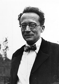
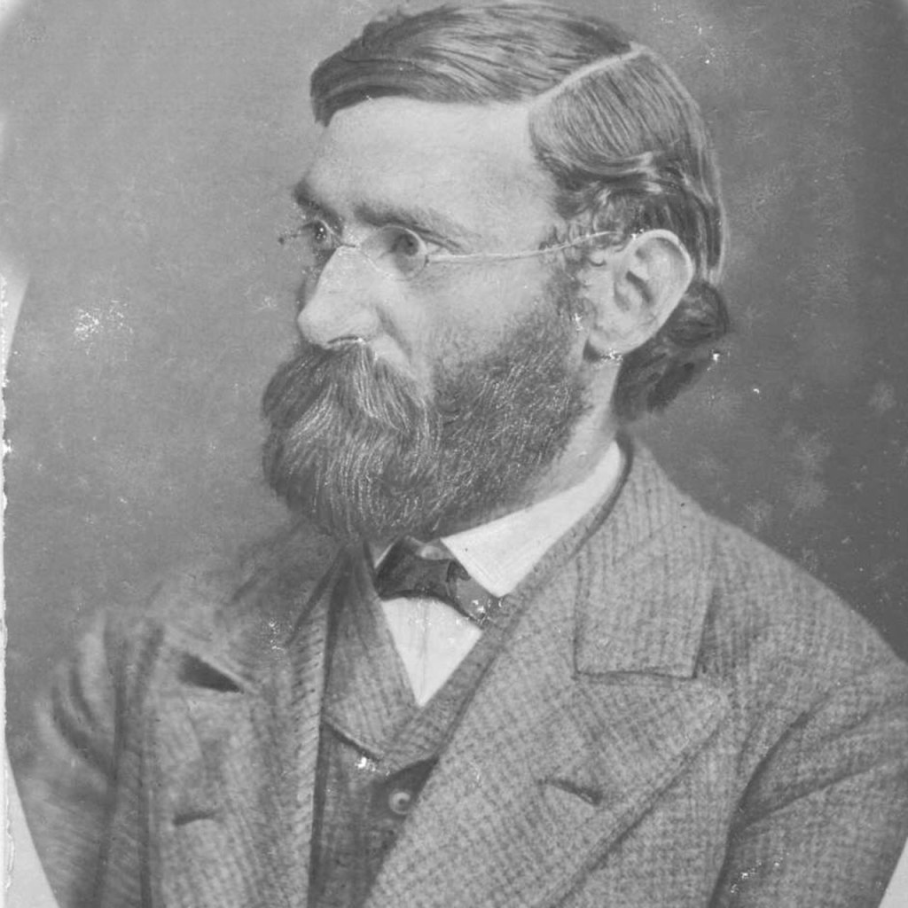
By the middle of 1925, a middle-aged Erwin Schrödinger was casting about, bogged down in mid career, looking for something significant to say about the rapidly accelerating field of quantum theory. He was known for his breadth of knowledge, and for his belief in his own creative genius [1], but a grand synthesis had so far eluded him.
Einsteinian Gas Theory
In the middle of the year, Schrödinger was deep analyzing two papers recently published by Einstein (Sept. 1924 and Feb. 1925) on the quantum properties of ideal gases where Einstein applied the new statistical theory of Bose to the counting of states in a volume of the gas [2]. One of the intriguing discoveries made by Einstein in those papers was a close analogy between the fluctuation of gas numbers and the interference of waves. He stated:
‘I believe that this is more than a mere analogy; de Broglie has shown in a very important work how a (scalar) wave field can be coordinated with a material particle or a system of material particles’
referring to de Broglie’s thesis work of 1924 that associated a wave-like property to mass. Einstein had been the first to attribute a wave-particle duality to the quantum phenomenon of black-body radiation, giving a lecture in Salzburg, Austria, in 1909 showing relationships between the particle-like and the wave-like properties of the radiation, and he found similar behavior in the properties of monatomic ideal gases, though his derivations were purely statistical.
Schrödinger was suspicious of the “unnatural” way of counting states used by Einstein and Bose for the gas, and he sought a more “natural” way of explaining how the elements of phase space were filled. It struck him that, just as Planck’s black-body radiation spectrum could be derived by assuming discrete standing-wave modes for the electromagnetic radiation, then perhaps the behavior of ideal gases could be obtained using a similar approach. He and Einstein exchanged several letters about this idea as Schrödinger dug deeper into de Broglie’s theory.
The Zurich Seminar
At that time, Schrödinger was in the Chair of Theoretical Physics at the University of Zurich, holding the same chair that Einstein had held 15 years earlier. Following Einstein, the chair had been occupied by Max von Laue and then by Peter Debye who moved to the ETH in Zurich. Debye organized a joint seminar between the University and ETH that was a hot social gathering of physicists and physical chemists, discussing the latest developments in atomic and quantum science.
In November of 2025, Debye, who probably knew about the Einstein-Schrödinger discussion on de Broglie, asked Schrödinger to give a seminar on de Broglie’s theory to the group. A young Felix Bloch, who was a graduate student at that time, recalled hearing Debye say something like
“Schrödinger, you are not working right now on very important problems anyway. Why don’t you tell us sometime about that thesis of de Broglie, which seems to have attracted some attention?”[3]
Schrödinger gave the overview seminar in early December, showing how the Bohr-Sommerfeld quantization conditions could be explained as standing waves using de Broglie’s theory, but Bloch recalled Debye was unimpressed, saying that de Broglie’s way of talking was “childish” and that what was needed for a proper physics theory was a wave equation.
This exchange between Schrödinger and Debye was recalled only in later years, and there is debate about what exactly was said and what effect it had on Schrödinger. From Schrödinger’s letters to friends, it is clear that he was already well into his investigations of wavelike properties of matter when Debye asked him to give the seminar. Furthermore, he had already tried to construct wave packets using superpositions of phase waves propagating along Bohr-Sommerfeld elliptical orbits but had been led to ugly caustics when he tried to apply the packets to the hydrogen atom [4]. Therefore, although Debye was probably not the source of Schrödinger’s interest in de Broglie, it is possible that Debye’s quip about “childishness” may have spurred Schrödinger to find a wave equation subject to boundary conditions rather than working with packets following ray paths.
The Christmas Breakthrough
By this time, Christmas was approaching and Schrödinger arranged to take a vacation away from his family to the Swiss Alpine village of Arosa, and given his unconventional belief in the link between personal pleasure and genius, he did not go alone. There is no record of what transpired, and no record of which mistress was with him on this particular trip, nor how she spent her time while he worked on his theory, but two days after Christmas he wrote a letter to the physicist Willy Wien saying
“At the moment I am struggling with a new atomic theory. If only I knew more mathematics! I am very optimistic about this thing, and expect that, if only I can . . . solve it, it will be very beautiful.. . . I hope that I can soon report in a little more detailed and understandable way about the matter. At present I must learn a little mathematics in order to completely solve the vibration problem …”[5]
He had uncovered his first wave equation. When he returned to Zurich, he enlisted the help of his friend, the mathematician Hermann Weyl at the University in Zurich, and Schrödinger had his first eigenfrequencies for hydrogen. But they were wrong!
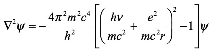
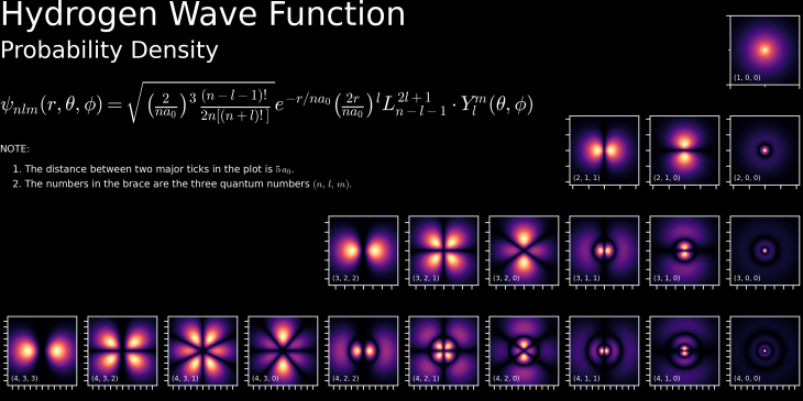
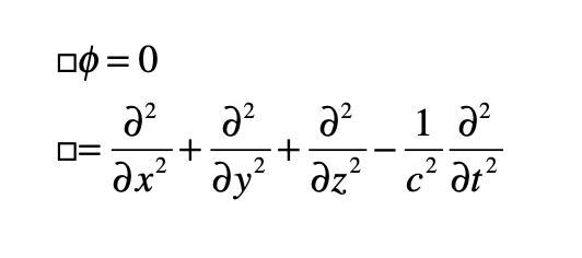
Fig. 2 Schrödinger’s first wave equation was relativistic.
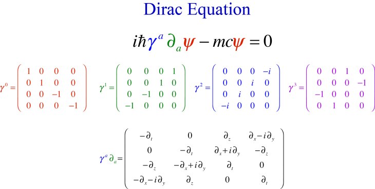
The theory of de Broglie was fundamentally a relativistic theory, motivated by mapping the behavior of matter onto the behavior of light. Therefore, Schrödinger’s first attempt was also relativistic, equivalent to the Klein-Gordon equation. But there was no clear understanding of electron spin at that time, even though it had been established as a fundamental property of the electron. It was only several years later when Dirac correctly accounted for electron spin in a relativistic wave equation.
Fig. 3 The full relativistic Dirac equation.
The Schrödinger Wave Equation
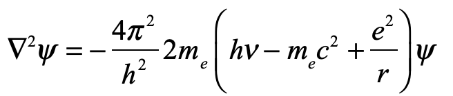
Convinced that he was onto something big, and unwilling to fail, despite his failure to obtain correct values for hydrogen, Schrödinger went back to first principles, to the classical theory of Hamiltonian mechanics, identifying Hamilton’s characteristic function with the phase of an electron wave and deriving a non-relativistic equation using variational principles subject to boundary conditions. The eigenvalues of this new equation, when applied to hydrogen, matched the Bohr spectrum perfectly!
Fig. 4. Schrödinger’s second wave equation was non-relativistic and correctly matched the Bohr energy levels of hydrogen.
It had been only a few weeks since Schrödinger had given his previous seminar to the Zurich group, but in January he gave his update, probably given with some degree of satisfaction, having Debye in attendance, showing his now-famous wave equation and the agreement with experiment. Schrödinger wrote up his theory and results and submitted his paper on January 27, 1926, to Annalen der Physik [6].
Schrödinger had been known, but not as a forefront thinker, despite what he believed about himself. Now he was a forefront thinker, vindicating his beliefs but not always on the right track. He continued his unconventional lifestyle, marginalizing him socially, and he resisted Max Born’s and Niels Bohr’s probabilistic interpretations of the meaning of his own quantum wavefunction, marginalizing him professionally. Yet his breakthrough gave him a platform, and his skeptical reactions to his colleague’s successes helped illuminate the nature of the new physics (“Schrödinger’s Cat” [7]) through the decades to follow.
Bibliography
A very large body of historical work exists on the discovery of the Schrödinger equation, partially fueled by the lack of first-person accounts on how he achieved it. There has been a lot of speculation and a lot of sleuthing to uncover his path of discovery. Several accounts differ mainly in the timing of when he derived his equations, although all agree on the sequence: that the relativistic equation preceded the non-relativistic one. Here is a small sampling of the literature:
• Hanle, P. A. (1977). “The Coming of Age of Erwin Schrödinger: His Quantum Statistics of Ideal Gases.” Archive for History of Exact Sciences, 17(2), 165–192. DOI: 10.1007/BF00328532.
• Hanle, P. A. (1979). “The Schrödinger‐Einstein correspondence and the sources of wave mechanics.” American Journal of Physics, 47(7), 644–648. DOI: 10.1119/1.11587.
• Mehra, Jagdish. “Erwin Schrödinger and the Rise of Wave Mechanics. II. The Creation of Wave Mechanics.” Foundations of Physics, vol. 17, no. 12, 1987, pp. 1141-1188.
• Renn, J. (2013). “Schrödinger and the Genesis of Wave Mechanics.” In W. L. Reiter & J. Yngvason (Eds.), Erwin Schrödinger – 50 Years After (pp. 9–36). Zurich: European Mathematical Society. DOI: 10.4171/121-1/2.
• Wessels, L. (1979). “Schrödinger’s Route to Wave Mechanics.” Studies in History and Philosophy of Science Part A, 10(4), 311–340.
Notes
[1] He led an unconventional lifestyle (some would say emotionally predatory) based on his belief in the personal origins of genius. Although this behavior presented significant social barriers to his career, he refused to abandon it.
[2] A. Enstein, ‘Quantentheorie des einatomigen idealen Gases’, Preuss. Ak. Wiss. Sitzb. (1924) pp. 261 – 267, and (1925), pp. 3-14.
[6] Schrödinger, Erwin. “Quantisierung als Eigenwertproblem (Erste Mitteilung).” Annalen Der Physik, vol. 384, no. 4, 1926, pp. 361-376.
[7] Schrödinger, E. (1935). “Die gegenwärtige Situation in der Quantenmechanik.” Naturwissenschaften 23: 807–812, 823–828, 844–849. Schrödinger, E. (1980). “The Present Situation in Quantum Mechanics: A Translation of Schrödinger’s ‘Cat Paradox’ Paper.” Proceedings of the American Philosophical Society 124 (5): 323–338. (Translated by J. D. Trimmer).
Read more in Books by David Nolte at Oxford University Press
Of all the audacious proposals made by Einstein, and there were many, this one takes the cake because it should be impossible.
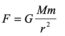
There can be no force of gravity on light because light has no mass. Without mass, there is no gravitational “interaction”. We all know Newton’s Law of gravity … it was one of the first equations of physics we ever learned
which shows the interaction between the masses M and m through their product. For light, this is strictly zero.
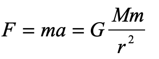
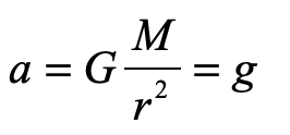
How, then did Einstein conclude, in 1907, only two years after he proposed his theory of special relativity, that gravity bends light? If it were us, we might take Newton’s other famous equation and equate the two
and guess that somehow the little mass m (though it equals zero) cancels out to give
so that light would fall in gravity with the same acceleration as anything else, massive or not.
But this is not how Einstein arrived at his proposal, because this derivation is wrong! To do it right, you have to think like an Einstein.
“My Happiest Thought”
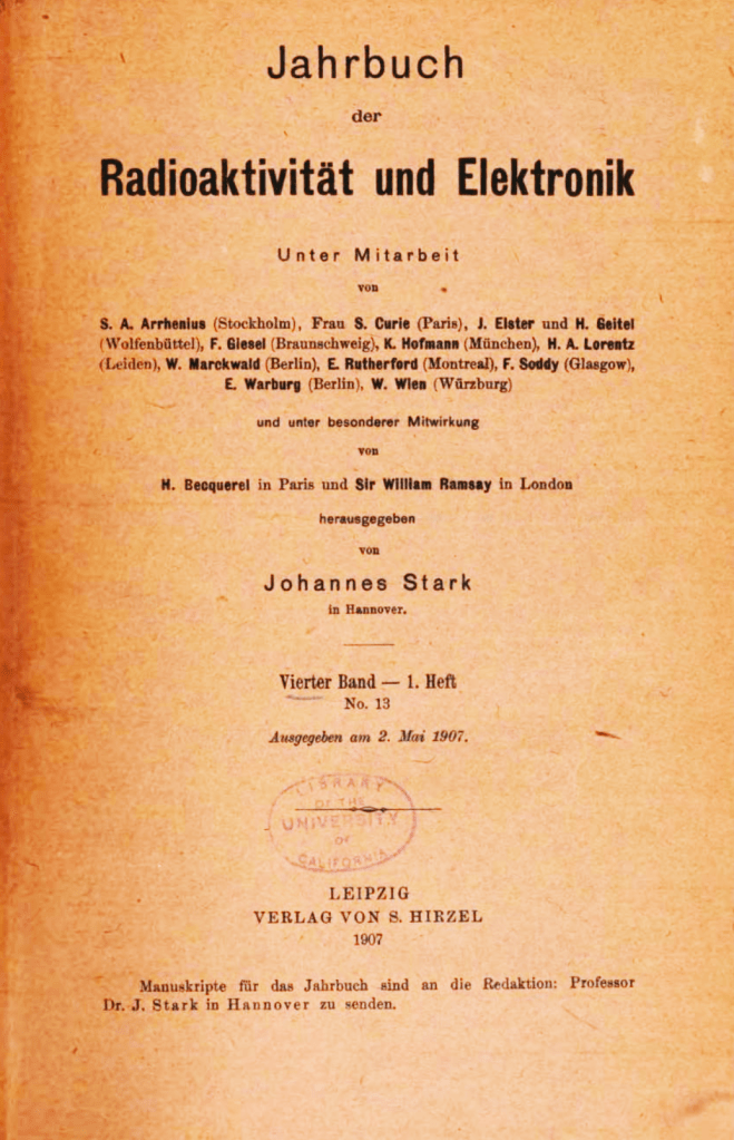
Towards the end of 1907, Einstein was asked by Johannes Stark to contribute a review article on the state of the relativity theory to the Jahrbuch of Radioactivity and Electronics. There had been a flurry of activity in the field in the two years since Einstein had published his groundbreaking paper in Annalen der Physik in September of 1905 [1]. Einstein himself had written several additional papers on the topic, along with others, so Stark felt it was time to put things into perspective.
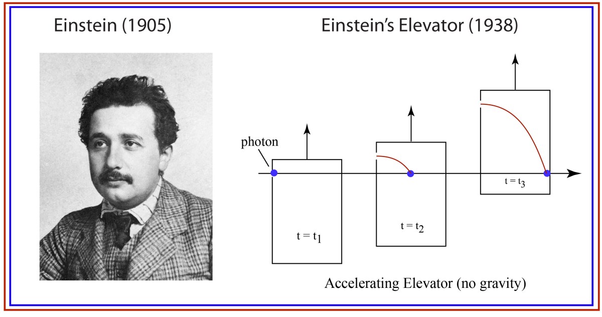
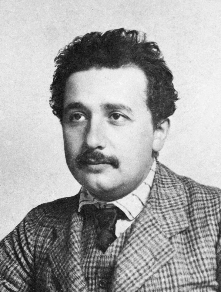
Fig. 1 Einstein around 1905.
Einstein was still working at the Patent Office in Bern, Switzerland, which must not have been too taxing, because it gave him plenty of time think. It was while he was sitting in his armchair in his office in 1907 that he had what he later described as the happiest thought of his life. He had been struggling with the details of how to apply relativity theory to accelerating reference frames, a topic that is fraught with conceptual traps, when he had a flash of simplifying idea:
“Then there occurred to me the ‘glucklichste Gedanke meines Lebens,’ the happiest thought of my life, in the following form. The gravitational field has only a relative existence in a way similar to the electric field generated by magnetoelectric induction. Because for an observer falling freely from the roof of a house there exists —at least in his immediate surroundings— no gravitational field. Indeed, if the observer drops some bodies then these remain relative to him in a state of rest or of uniform motion… The observer therefore has the right to interpret his state as ‘at rest.'”[2]
In other words, the freely falling observer believes he is in an inertial frame rather than an accelerating one, and by the principle of relativity, this means that all the laws of physics in the accelerating frame must be the same as for an inertial frame. Hence, his great insight was that there must be complete equivalence between a mechanically accelerating frame and a gravitational field. This is the very first conception of his Equivalence Principle.
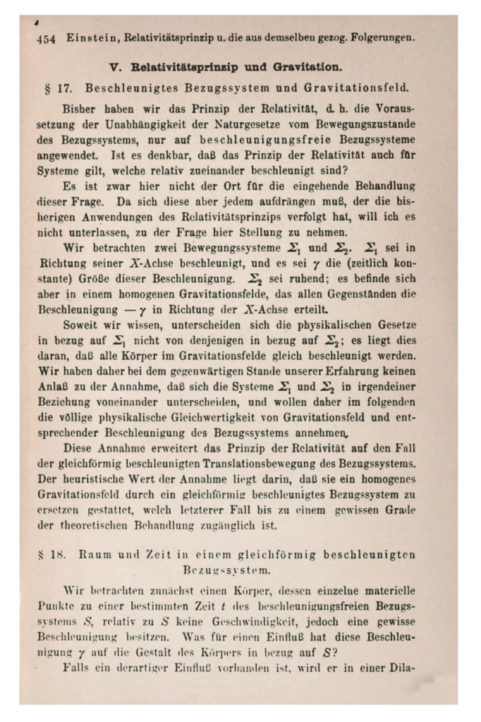
Fig. 2 Front page of the 1907 volume of the Jahrbuch. The editor list reads like a “Whos-Who” of early modern physics.
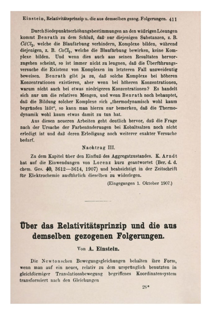
After completing his review of the consequences of special relativity in his Jahrbuch article, Einstein took the opportunity to launch into his speculations on the role of the relativity principle in gravitation. He is almost appologetic at the start, saying that:
“This is not the place for a detailed discussion of this question. But as it will occur to anybody who has been following the applications of the principle of relativity, I will not refrain from taking a stand on this question here.”
But he then launches into his first foray into general relativity with keen insights.
Fig. 4 The beginning of the section where Einstein first discusses the effects of accelerating frames and effects of gravity.
He states early in his exposition:
“… in the discussion that follows, we shall therefore assume the complete physical equivalence of a gravitational field and a corresponding accelerated reference system.”
Here is his equivalence principle. And using it, in 1907, he derives the effect of acceleration (and gravity) on ticking clocks, on the energy density of electromagnetic radiation (photons) in a gravitational potential, and on the deflection of light by gravity.
Over the next several years, Einstein was distracted by other things, such as obtaining his first university position, and his continuing work on the early quantum theory. But by 1910 he was ready to tackle the general theory of relativity once again, when he discovered that his equivalence principle was missing a key element: the effects of spatial curvature, which launched him on a 5-year program into the world of tensors and metric spaces that culminated with his completed general theory of relativity that he published in November of 1915 [4].
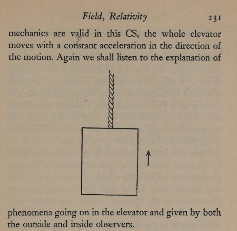
The Observer in the Chest: There is no Elevator
Einstein was never a stone to gather moss. Shortly after delivering his triumphal exposition on the General Theory of Relativity, he wrote up a popular account of his Special and now General Theories to be published as a book in 1916, first in German [5] and then in English [6]. What passed for a “popular exposition” in 1916 is far from what is considered popular today. Einstein’s little book is full of equations that would be somewhat challenging even for specialists. But the book also showcases Einstein’s special talent to create simple analogies, like the falling observer, that can make difficult concepts of physics appear crystal clear.
In 1916, Einstein was not yet thinking in terms of an elevator. His mental image at this time, for a sequestered observer, was someone inside a spacious chest filled with measurement apparatus that the observer could use at will. This observer in his chest was either floating off in space far from any gravitating bodies, or the chest was being pulled by a rope hooked to the ceiling such that the chest accelerates constantly. Based on the measurement he makes, he cannot distinguish between gravitational fields and acceleration, and hence they are equivalent. A bit later in the book, Einstein describes what a ray of light would do in an accelerating frame, but he does not have his observer attempt any such measurement, even in principle, because the deflection of the ray of light from a linear path would be far too small to measure.
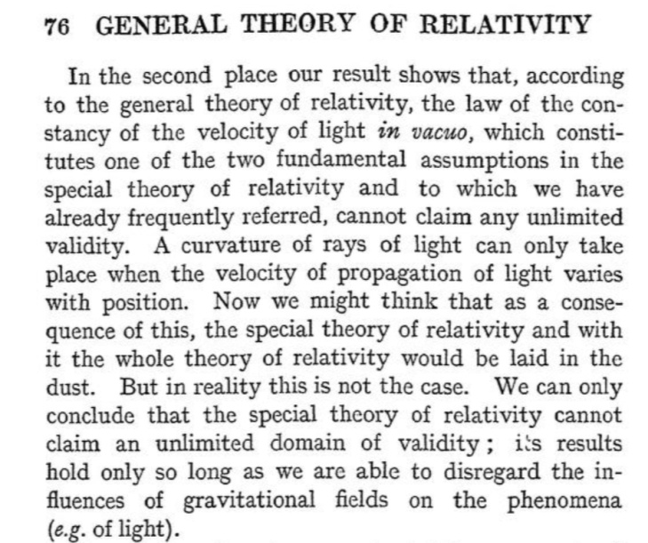
But Einstein does go on to say that any curvature of the path of the light ray requires that the speed of light changes with position. This is a shocking admission, because his fundamental postulate of relativity from 1905 was the invariance of the speed of light in all inertial frames. It was from this simple assertion that he was eventually able to derive E = mc2. Where, on the one hand, he was ready to posit the invariance of the speed of light, on the other hand, as soon as he understood the effects of gravity on light, Einstein did not hesitate to cast this postulate adrift.
Fig. 5 Einstein’s argument for the speed of light depending on position in a gravitational field.
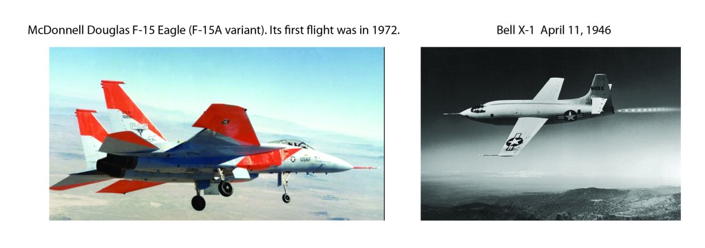
(Einstein can be forgiven for taking so long to speak in terms of an elevator that could accelerate at a rate of one g, because it was not until 1946 that the rocket plane Bell X-1 achieved linear acceleration exceeding 1 g, and jet planes did not achieve 1 g linear acceleration until the F-15 Eagle in 1972.)
Fig. 6 Aircraft with greater than 1:1 thrust to weight ratios.
The Evolution of Physics: Enter Einstein’s Elevator
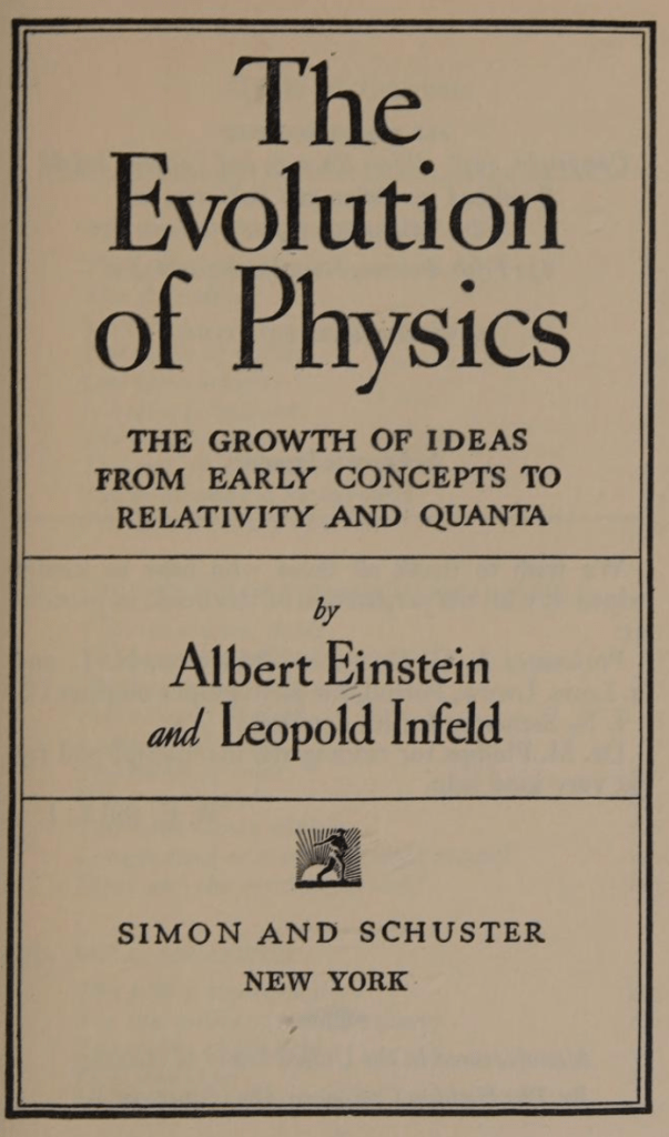
Years passed, and Einstein fled an increasingly autocratic and belligerent Germany for a position at Princeton’s Institute for Advanced Study. In 1938, at the instigation of his friend Leopold Infeld, they decided to write a general interest book on the new physics of relativity and quanta that had evolved so rapidly over the past 30 years.
Fig. 7 Title page of “Evolution of Physics” 1938 written with his friend Leopold Infeld at Princeton’s Institute for Advanced Study.
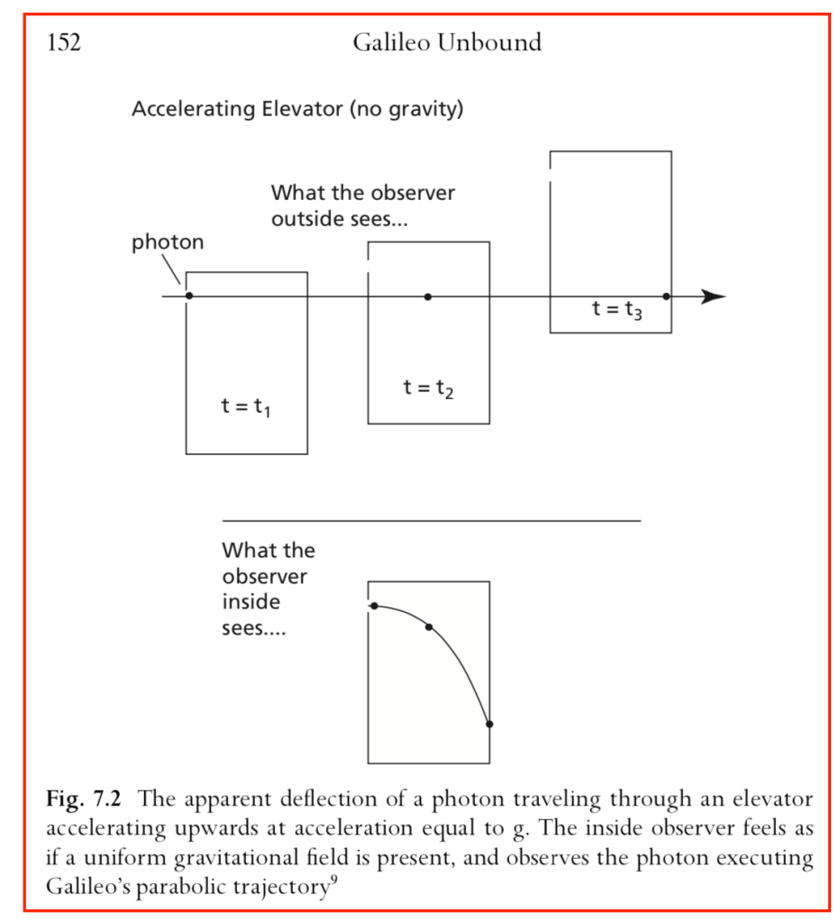
Here, in this obscure book that no-one remembers today, we find Einstein’s elevator for the first time, and the exposition talks very explicitly about a small window that lets in a light ray, and what the observer sees (in principle) for the path of the ray.
Fig. 8 One of the only figures in the Einstein and Infeld book: The origin of “Einstein’s Elevator”!
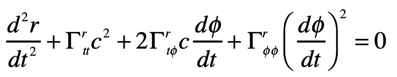
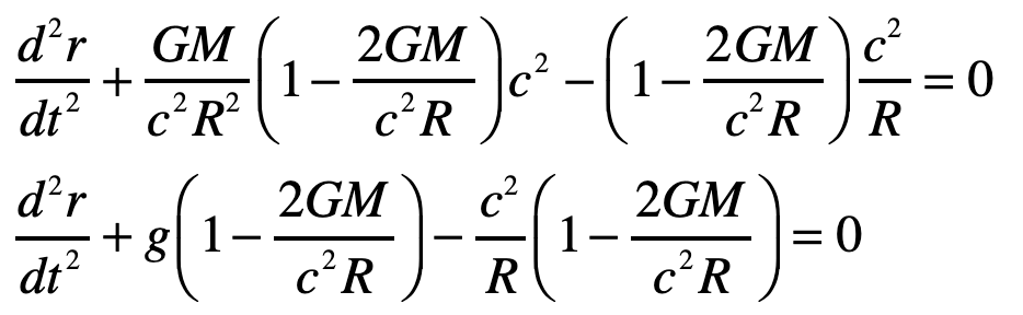
By the equivalence principle, the observer cannot tell whether they are far out in space, being accelerated at the rate g, or whether they are statinary on the surface of the Earth subject to a gravitational field. In the first instance of the accelerating elevator, a photon moving in a straight line through space would appear to deflect downward in the elevator, as shown in Fig. 9, because the elevator is accelerating upwards as the photon transits the elevator. However, by the equivalence principle, the same physics should occur in the gravitational field. Hence, gravity must bend light. Furthermore, light falls inside the elevator with an acceleration g, just as any other object would.
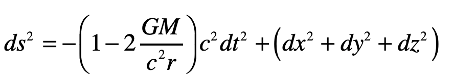
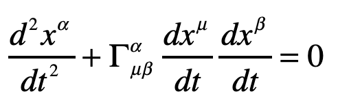
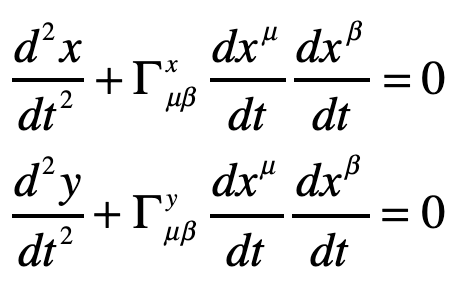
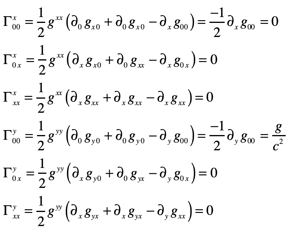
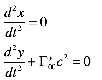
A photon enters an elevator at right angles to its acceleration vector g. Use the geodesic equation and the elevator (Equivalence Principle) metric [8]
The geodesic equation with time as the dependent variable
This gives two coordinate equations
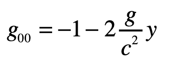
Note that x0 = ct and x1 = ct are both large relative to the y-motion of the photon. The metric component that is relevant here is
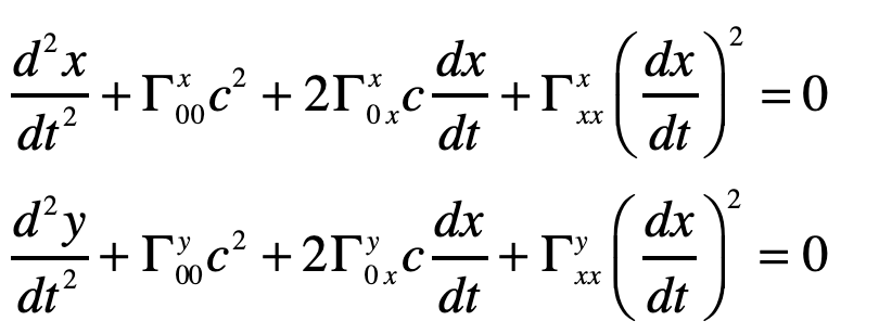
and the others are unity. The geodesic becomes (assuming dy/dt = 0)
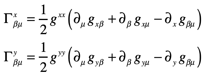
The Christoffel symbols are
which give
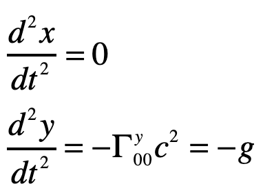
Therefore
or
where the photon falls with acceleration g, as anticipated.
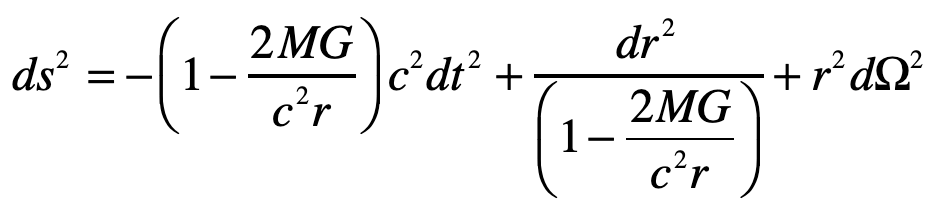
Light Deflection in the Schwarzschild Metric
Do the same problem of the light ray in Einstein’s Elevator, but now using the full Schwarzschild solution to the Einstein Field equations.
Solution:
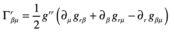
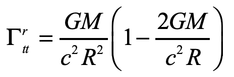
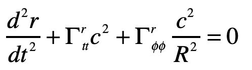
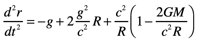
Einstein’s elevator is the classic test of virtually all heuristic questions related to the deflection of light by gravity. In the previous Example, the deflection was attributed to the Equivalence Principal in which the observer in the elevator cannot discern whether they are in an acceleration rocket ship or standing stationary on Earth. In that case, the time-like metric component is the sole cause of the free-fall of light in gravity. In the Schwarzschild metric, on the other hand, the curvature of the field near a spherical gravitating body also contributes. In this case, the geodesic equation, assuming that dr/dt = 0 for the incoming photon, is
where, as before, the Christoffel symbol for the radial displacements are
Evaluating one of these
The other Christoffel symbol that contributes to the radial motion is
and the geodesic equation becomes
with
The radial acceleration of the light ray in the elevator is thus
The first term on right is free-fall in gravity, just as was obtained from the Equivalence Principal. The second term is a higher-order correction caused by curvature of spacetime. The third term is the motion of the light ray relative to the curved ceiling of the elevator in this spherical geometry and hence is a kinematic (or geometric) artefact. (It is interesting that the GR correction on the curved-ceiling correction is of the same order as the free-fall term, so one would need to be very careful doing such an experiment … if it were at all measurable.) Therefore, the second and third terms are curved-geometry effects while the first term is the free fall of the light ray.
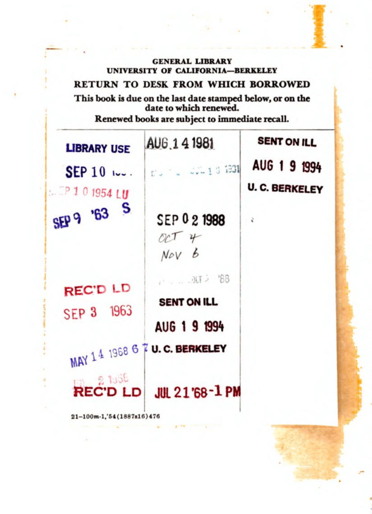
Post-Script: The Importance of Library Collections
I was amused to see the library card of the scanned Internet Archive version of Einstein’s Jahrbuch article, shown below. The volume was checked out in August of 1981 from the UC Berkeley Physics Library. It was checked out again 7 years later in September of 1988. These dates coincide with when I arrived at Berkeley to start grad school in physics, and when I graduated from Berkeley to start my post-doc position at Bell Labs. Hence this library card serves as the book ends to my time in Berkeley, a truly exhilarating place that was the top-ranked physics department at that time, with 7 active Nobel Prize winners on its faculty.
During my years at Berkeley, I scoured the stacks of the Physics Library looking for books and journals of historical importance, and was amazed to find the original volumes of Annalen der Physik from 1905 where Einstein published his famous works. This was the same library where, ten years before me, John Clauser was browsing the stacks and found the obscure paper by John Bell on his inequalities that led to Clauser’s experiment on entanglement that won him the Nobel Prize of 2022.
That library at UC Berkeley was recently closed, as was the Physics Library in my department at Purdue University (see my recent Blog), where I also scoured the stacks for rare gems. Some ancient books that I used to be able to check out on a whim, just to soak up their vintage ambience and to get a tactile feel for the real thing held in my hands, are now not even available through Interlibrary Loan. I may be able to get scans from Internet Archive online, but the palpable magic of the moment of discovery is lost.
References:
[1] Einstein, A. (1905). Zur Elektrodynamik bewegter Körper. Annalen der Physik, 17(10), 891–921.
[2] Pais, A (2005). Subtle is the Lord: The Science and Life of Albert Einstein (Oxford University Press). pg. 178
[3] Einstein, A. (1907). Über das Relativitätsprinzip und die aus demselben gezogenen Folgerungen. Jahrbuch der Radioaktivität und Elektronik, 4, 411–462.
[4] A. Einstein (1915), “On the general theory of relativity,” Sitzungsberichte Der Koniglich Preussischen Akademie Der Wissenschaften, pp. 778-786, Nov.
[5] Einstein, A. (1916). Über die spezielle und die allgemeine Relativitätstheorie (Gemeinverständlich). Braunschweig: Friedr. Vieweg & Sohn.
[6] Einstein, A. (1920). Relativity: The Special and the General Theory (A Popular Exposition) (R. W. Lawson, Trans.). London: Methuen & Co. Ltd.
At the turn of the New Year, as I turn to the breakthroughs in physics of the previous year, sifting through the candidates, I usually narrow it down to about 4 to 6 that I find personally compelling (See, for instance 2023, 2022). In a given year, they may be related to things like supersolids, condensed atoms, or quantum entanglement. Often they relate to those awful, embarrassing gaps in physics knowledge that we give euphemistic names to, like “Dark Energy” and “Dark Matter” (although in the end they may be neither energy nor matter). But this year, as I sifted, I was struck by how many of the “physics” advances of the past year were focused on pushing limits—lower temperatures, more qubits, larger distances.
If you want something that is eventually useful, then engineering is the way to go, and many of the potential breakthroughs of 2024 did require heroic efforts. But if you are looking for a paradigm shift—a new way of seeing or thinking about our reality—then bigger, better and farther won’t give you that. We may be pushing the boundaries, but the thinking stays the same.
Therefore, for 2024, I have replaced “breakthrough” with a single “prospect” that may force us to change our thinking about the universe and the fundamental forces behind it.
This prospect is the weakening of dark energy over time.
It is a “prospect” because it is not yet absolutely confirmed. If it is confirmed in the next few years, then it changes our view of reality. If it is not confirmed, then it still forces us to think harder about fundamental questions, pointing where to look next.
Einstein’s Cosmological “Constant”
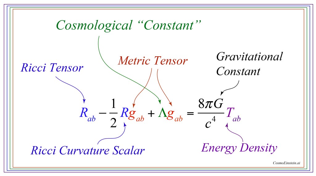
Like so much of physics today, the origins of this story go back to Einstein. At the height of WWI in 1917, as Einstein was working in Berlin, he “tweaked” his new theory of general relativity to allow the universe to be static. The tweak came in the form of a parameter he labelled Lambda (Λ), providing a counterbalance against the gravitational collapse of the universe, which at the time was assumed to have a time-invariant density. This cosmological “constant” of spacetime represented a pressure that kept the universe inflated like a balloon.
Fig. 1 Einstein’s “Field Equations” for the universe containing expressions for curvature, the metric tensor and energy density. Spacetime is warped by energy density, and trajectories within the warped spacetime follow geodesic curves. When Λ = 0, only gravitional attraction is present. When Λ ≠ 0, a “repulsive” background force exerts a pressure on spacetime, keeping it inflated like a balloon.
Later, in 1929 when Edwin Hubble discovered that the universe was not static but was expanding, and not only expanding, but apparently on a free trajectory originating at some point in the past (the Big Bang), Einstein zeroed out his cosmological constant, viewing it as one of his greatest blunders.
And so it stood until 1998 when two teams announced that the expansion of the universe is accelerating—and Einstein’s cosmological constant was back in. In addition, measurements of the energy density of the universe showed that the cosmological constant was contributing around 68% of the total energy density, which has been given the name of Dark Energy. One of the ways to measure Dark Energy is through BAO.
Baryon Acoustic Oscillations (BAO)
If the goal of science communication is to be transparent, and to engage the public in the heroic pursuit of pure science, then the moniker Baryon Acoustic Oscillations (BAO) was perhaps the wrong turn of phrase. “Cosmic Ripples” might have been a better analogy (and a bit more poetic).
In the early moments after the Big Bang, slight density fluctuations set up a balance of opposing effects between gravitational attraction, that tends to clump matter, and the homogenization effects of the hot photon background, that tends to disperse ionized matter. Matter consists of both dark matter as well as the matter we are composed of, known as baryonic matter. Only baryonic matter can be ionized and hence interact with photons, hence only photons and baryons experience this balance. As the universe expanded, an initial clump of baryons and photons expanded outward together, like the ripples on a millpond caused by a thrown pebble. And because the early universe had many clumps (and anti-clumps where density was lower than average), the millpond ripples were like those from a gentle rain with many expanding ringlets overlapping.
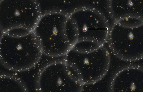
Fig. 2 Overlapping ripples showing galaxies formed along the shells. The size of the shells is set by the speed of “sound” in the universe. From [Ref].
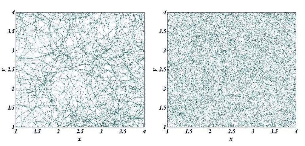
Fig. 3 Left. Galaxies formed on acoustic ringlets like drops of dew on a spider’s web. Right. Many ringlets overlapping. The characteristic size of the ringlets can still be extracted statistically. From [Ref].
Then, about 400,000 years after the Big Bang, as the universe expanded and cooled, it got cold enough that ionized electrons and baryons formed atoms that are neutral and transparent to light. Light suddenly flew free, decoupled from the matter that had constrained it. Removing the balance between light and matter in the BAO caused the baryonic ripples to freeze in place, as if a sudden arctic blast froze the millpond in an instant. The residual clumps of matter in the early universe became clumps of galaxies in the modern universe that we can see and measure. We can also see the effects of those clumps on the temperature fluctuations of the cosmic microwave background (CMB).
Between these two—the BAO and the CMB—it is possible to measure cosmic distances, and with those distances, to measure how fast the universe is expanding.
Acceleration Slowing
The Dark Energy Spectroscopic Instrument (DESI) on top of Kitt Peak in Arizona is measuring the distances to millions of galaxies using automated fiber optic arrays containing thousands of optical fibers. In one year it measured the distances to about 6 milliion galaxies.
Fig. 4 The Kitt Peak observatory, the site of DESI. From [Ref].
By focusing on seven “epochs” in galaxy formation in the universe, it measures the sizes of the BAO ripples over time, ranging in ages from 3 billion to 11 billion years ago. (The universe is about 13.8 billion years old.) The relative sizes are then compared to the predictions of the LCDM (Lambda-Cold-Dark-Matter) model. This is the “consensus” model of the day—agreed upon as being “most likely” to explain observations. If Dark Energy is a true constant, then the relative sizes of the ripples should all be the same, regardless of how far back in time we look.
But what the DESI data discovered is that relative sizes more recently (a few billion years ago) are smaller than predicted by LCDM. Given that LCDM includes the acceleration of the expansion of the universe caused by Dark Energy, it means that Dark Energy is slightly weaker in the past few billion years than it was 10 billion years ago—it’s weakening or “thawing”.
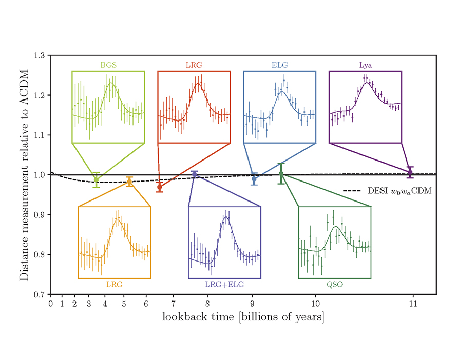
The measurements as they stand today are shown in Fig. 5, showing the relative sizes as a function of how far back in time they look, with a dashed line showing the deviation from the LCDM prediction. The error bars in the figure are not yet are that impressive, and statistical effects may be causing the trend, so it might be erased by more measurements. But the BAO results have been augmented by recent measurements of supernova (SNe) that provide additional support for thawing Dark Energy. Combined, the BAO+SNe results currently stand at about 3.4 sigma. The gold standard for “discovery” is about 5 sigma, so there is still room for this effect to disappear. So stay tuned—the final answer may be known within a few years.
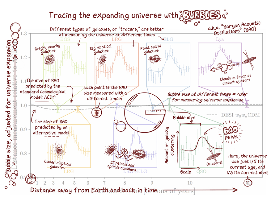
Fig. 5 Seven “epochs” in the evolution of galaxies in the universe. This plot shows relative galactic distances as a function of time looking back towards the Big Bang (older times closer to the Big Bang are to the right side of the graph). In more recent times, relative distances are smaller than predicted by the consensus theory known as Lambda-Cold-Dark-Matter (LCDM), suggesting that Dark Energy is slight weaker today than it was billions of years ago. The three left-most data points (with error bars from early 2024) are below the LCDM line. From [Ref].Fig. 6 Annotated version of the previous figure. From [Ref].
The Future of Physics
The gravitational constant G is considered to be a constant property of nature, as is Planck’s constant h, and the charge of the electron e. None of these fundamental properties of physics are viewed as time dependent and none can be derived from basic principles. They are simply constants of our reality. But if Λ is time dependent, then it is not a fundamental constant and should be derivable and explainable.
Light is one of the most powerful manifestations of the forces of physics because it tells us about our reality. The interference of light, in particular, has led to the detection of exoplanets orbiting distant stars, discovery of the first gravitational waves, capture of images of black holes and much more. The stories behind the history of light and interference go to the heart of how scientists do what they do and what they often have to overcome to do it. These time-lines are organized along the chapter titles of the book Interference. They follow the path of theories of light from the first wave-particle debate, through the personal firestorms of Albert Michelson, to the discoveries of the present day in quantum information sciences.
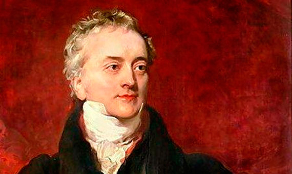
Thomas Young was the ultimate dabbler, his interests and explorations ranged far and wide, from ancient egyptology to naval engineering, from physiology of perception to the physics of sound and light. Yet unlike most dabblers who accomplish little, he made original and seminal contributions to all these fields. Some have called him the “Last Man Who Knew Everything“.
Thomas Young. The Law of Interference.
Topics: The Law of Interference. The Rosetta Stone. Benjamin Thompson, Count Rumford. Royal Society. Christiaan Huygens. Pendulum Clocks. Icelandic Spar. Huygens’ Principle. Stellar Aberration. Speed of Light. Double-slit Experiment.
1629 – Huygens born (1629 – 1695)
1642 – Galileo dies, Newton born (1642 – 1727)
1655 – Huygens ring of Saturn
1657 – Huygens patents the pendulum clock
1666 – Newton prismatic colors
1666 – Huygens moves to Paris
1669 – Bartholin double refraction in Icelandic spar
1670 – Bartholinus polarization of light by crystals
1671 – Expedition to Hven by Picard and Rømer
1673 – James Gregory bird-feather diffraction grating
1801 – Young Theory of Light and Colours, three color mechanism (Bakerian Lecture), Young considers interference to cause the colored films, first estimates of the wavelengths of different colors
1802 – Young begins series of lecturs at the Royal Institution (Jan. 1802 – July 1803)
1802 – Young names the principle (Law) of interference
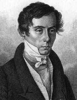
Augustin Fresnel was an intuitive genius whose talents were almost squandered on his job building roads and bridges in the backwaters of France until he was discovered and rescued by Francois Arago.
Topics: Particles versus Waves. Malus and Polarization. Agustin Fresnel. Francois Arago. Diffraction. Daniel Bernoulli. The Principle of Superposition. Joseph Fourier. Transverse Light Waves.
1665 – Grimaldi diffraction bands outside shadow
1673 – James Gregory bird-feather diffraction grating
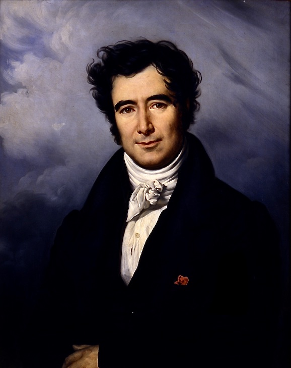
There is no question that Francois Arago was a swashbuckler. His life’s story reads like an adventure novel as he went from being marooned in hostile lands early in his career to becoming prime minister of France after the 1848 revolutions swept across Europe.
Topics: The Birth of Interferometry. Snell’s Law. Fresnel and Arago. The First Interferometer. Fizeau and Foucault. The Speed of Light. Ether Drag. Jamin Interferometer.
No name is more closely connected to interferometry than that of Albert Michelson. He succeeded, sometimes at great personal cost, in launching interferometric metrology as one of the most important tools used by scientists today.
Albert A. Michelson, 1907 Nobel Prize. Image Credit.
Topics: The Trials of Albert Michelson. Hermann von Helmholtz. Michelson and Morley. Fabry and Perot.
1810 – Arago search for ether drag
1813 – Fraunhofer dark lines in Sun spectrum
1813 – Faraday begins at Royal Institution
1820 – Oersted discovers electromagnetism
1821 – Faraday electromagnetic phenomena
1827 – Green mathematical analysis of electricity and magnetism
1830 – Cauchy ether as elastic solid
1831 – Faraday electromagnetic induction
1831 – Cauchy ether drag
1831 – Maxwell born
1831 – Faraday electromagnetic induction
1836 – Cauchy’s second theory of the ether
1838 – Green theory of the ether
1839 – Hamilton group velocity
1839 – MacCullagh properties of rotational ether
1839 – Cauchy ether with negative compressibility
1841 – Maxwell entered Edinburgh Academy (age 10) met P. G. Tait
1842 – Doppler effect
1845 – Faraday effect (magneto-optic rotation)
1846 – Stokes’ viscoelastic theory of the ether
1847 – Maxwell entered Edinburgh University
1850 – Maxwell at Cambridge, studied under Hopkins, also knew Stokes and Whewell
1852 – Michelson born Strelno, Prussia
1854 – Maxwell wins the Smith’s Prize (Stokes’ theorem was one of the problems)
1855 – Michelson’s immigrate to San Francisco through Panama Canal
Learning from his attempts to measure the speed of light through the ether, Michelson realized that the partial coherence of light from astronomical sources could be used to measure their sizes. His first measurements using the Michelson Stellar Interferometer launched a major subfield of astronomy that is one of the most active today.
R Hanbury Brown
Topics: Measuring the Stars. Astrometry. Moons of Jupiter. Schwarzschild. Betelgeuse. Michelson Stellar Interferometer. Banbury Brown Twiss. Sirius. Adaptive Optics.
1838 – Bessel stellar parallax measurement with Fraunhofer telescope
1868 – Fizeau proposes stellar interferometry
1873 – Stephan implements Fizeau’s stellar interferometer on Sirius, sees fringes
1880 – Michelson Idea for second-order measurement of relative motion against ether
1880 – 1882 Michelson Studies in Europe (Helmholtz in Berlin, Quincke in Heidelberg, Cornu, Mascart and Lippman in Paris)
1881 – Michelson Measurement at Potsdam with funds from Alexander Graham Bell
1881 – Michelson Resigned from active duty in the Navy
1883 – Michelson Joined Case School of Applied Science
1889 – Michelson moved to Clark University at Worcester
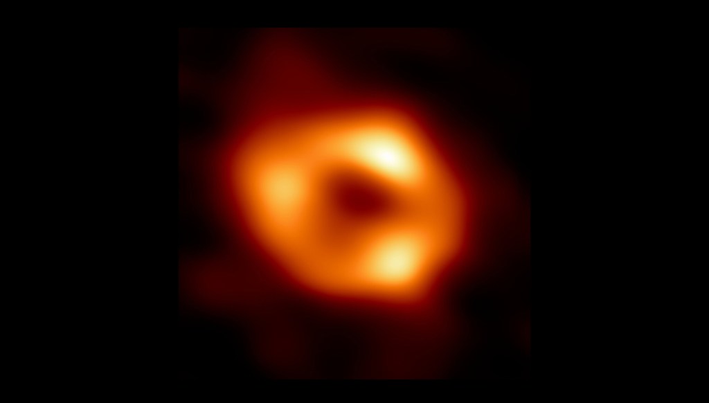
Stellar interferometry is opening new vistas of astronomy, exploring the wildest occupants of our universe, from colliding black holes half-way across the universe (LIGO) to images of neighboring black holes (EHT) to exoplanets near Earth that may harbor life.
Image of the supermassive black hole in M87 from Event Horizon Telescope.
Topics: Gravitational Waves, Black Holes and the Search for Exoplanets. Nulling Interferometer. Event Horizon Telescope. M87 Black Hole. Long Baseline Interferometry. LIGO.
1947 – Virgo A radio source identified as M87
1953 – Horace W. Babcock proposes adaptive optics (AO)
From the astronomically large dimensions of outer space to the microscopically small dimensions of inner space, optical interference pushes the resolution limits of imaging.
Topics: Diffraction and Interference. Joseph Fraunhofer. Diffraction Gratings. Henry Rowland. Carl Zeiss. Ernst Abbe. Phase-contrast Microscopy. Super-resolution Micrscopes. Structured Illumination.
The coherence of laser light is like a brilliant jewel that sparkles in the darkness, illuminating life, probing science and projecting holograms in virtual worlds.
What is the image of one photon interfering? Better yet, what is the image of two photons interfering? The answer to this crucial question laid the foundation for quantum communication.
Topics: The Beginnings of Quantum Communication. EPR paradox. Entanglement. David Bohm. John Bell. The Bell Inequalities. Leonard Mandel. Single-photon Interferometry. HOM Interferometer. Two-photon Fringes. Quantum cryptography. Quantum Teleportation.
1900 – Planck (1901). “Law of energy distribution in normal spectra.” [1]
There is almost no technical advantage better than having exponential resources at hand. The exponential resources of quantum interference provide that advantage to quantum computing which is poised to usher in a new era of quantum information science and technology.
David Deutsch.
Topics: Interferometric Computing. David Deutsch. Quantum Algorithm. Peter Shor. Prime Factorization. Quantum Logic Gates. Linear Optical Quantum Computing. Boson Sampling. Quantum Computational Advantage.
1980 – Paul Benioff describes possibility of quantum computer
[10] B. R. Mollow, R. J. Glauber: Phys. Rev. 160, 1097 (1967); 162, 1256 (1967)
[11] J. F. Clauser, M. A. Horne, A. Shimony, and R. A. Holt, ” Proposed experiment to test local hidden-variable theories,” Physical Review Letters, vol. 23, no. 15, pp. 880-&, (1969)
[15] R. Ghosh and L. Mandel, “Observation of nonclassical effects in the interference of 2 photons,” Physical Review Letters, vol. 59, no. 17, pp. 1903-1905, Oct (1987)
[16] C. K. Hong, Z. Y. Ou, and L. Mandel, “Measurement of subpicosecond time intervals between 2 photons by interference,” Physical Review Letters, vol. 59, no. 18, pp. 2044-2046, Nov (1987)
[18] D. Deutsch, “QUANTUM-THEORY, THE CHURCH-TURING PRINCIPLE AND THE UNIVERSAL QUANTUM COMPUTER,” Proceedings of the Royal Society of London Series a-Mathematical Physical and Engineering Sciences, vol. 400, no. 1818, pp. 97-117, (1985)
[19] P. W. Shor, “ALGORITHMS FOR QUANTUM COMPUTATION – DISCRETE LOGARITHMS AND FACTORING,” in 35th Annual Symposium on Foundations of Computer Science, Proceedings, S. Goldwasser Ed., (Annual Symposium on Foundations of Computer Science, 1994, pp. 124-134.
[20] F. Arute et al., “Quantum supremacy using a programmable superconducting processor,” Nature, vol. 574, no. 7779, pp. 505-+, Oct 24 (2019)
[21] H.-S. Zhong et al., “Quantum computational advantage using photons,” Science, vol. 370, no. 6523, p. 1460, (2020)
Further Reading: The History of Light and Interference (2023)
The first step on the road to Einstein’s relativity was taken a hundred years earlier by an ironic rebel of physics—Augustin Fresnel. His radical (at the time) wave theory of light was so successful, especially the proof that it must be composed of transverse waves, that he was single-handedly responsible for creating the irksome luminiferous aether that would haunt physicists for the next century. It was only when Einstein combined the work of Fresnel with that of Hippolyte Fizeau that the aether was ultimately banished.
Augustin Fresnel: Ironic Rebel of Physics
Augustin Fresnel was an odd genius who struggled to find his place in the technical hierarchies of France. After graduating from the Ecole Polytechnique, Fresnel was assigned a mindless job overseeing the building of roads and bridges in the boondocks of France—work he hated. To keep himself from going mad, he toyed with physics in his spare time, and he stumbled on inconsistencies in Newton’s particulate theory of light that Laplace, a leader of the French scientific community, embraced as if it were revealed truth .
The final irony is that Einstein used Fresnel’s theoretical coefficient and Fizeau’s measurements—that had introduced aether drag in the first place—to show that there was no aether.
Fresnel rebelled, realizing that effects of diffraction could be explained if light were made of waves. He wrote up an initial outline of his new wave theory of light, but he could get no one to listen, until Francois Arago heard of it. Arago was having his own doubts about the particle theory of light based on his experiments on stellar aberration.
Augustin Fresnel and Francois Arago (circa 1818)
Stellar Aberration and the Fresnel Drag Coefficient
Stellar aberration had been explained by James Bradley in 1729 as the effect of the motion of the Earth relative to the motion of light “particles” coming from a star. The Earth’s motion made it look like the star was tilted at a very small angle (see my previous blog). That explanation had worked fine for nearly a hundred years, but then around 1810 Francois Arago at the Paris Observatory made extremely precise measurements of stellar aberration while placing finely ground glass prisms in front of his telescope. According to Snell’s law of refraction, which depended on the velocity of the light particles, the refraction angle should have been different at different times of the year when the Earth was moving one way or another relative to the speed of the light particles. But to high precision the effect was absent. Arago began to question the particle theory of light. When he heard about Fresnel’s work on the wave theory, he arranged a meeting, encouraging Fresnel to continue his work.
But at just this moment, in March of 1815, Napoleon returned from exile in Elba and began his march on Paris with a swelling army of soldiers who flocked to him. Fresnel rebelled again, joining a royalist militia to oppose Napoleon’s return. Napoleon won, but so did Fresnel, who was ironically placed under house arrest, which was like heaven to him. It freed him from building roads and bridges, giving him free time to do optics experiments in his mother’s house to support his growing theoretical work on the wave nature of light.
Arago convinced the authorities to allow Fresnel to come to Paris, where the two began experiments on diffraction and interference. By using polarizers to control the polarization of the interfering light paths, they concluded that light must be composed of transverse waves.
This brilliant insight was then followed by one of the great tragedies of science—waves needed a medium within which to propagate, so Fresnel conceived of the luminiferous aether to support it. Worse, the transverse properties of light required the aether to have a form of crystalline stiffness.
How could moving objects, like the Earth orbiting the sun, travel through such an aether without resistance? This was a serious problem for physics. One solution was that the aether was entrained by matter, so that as matter moved, the aether was dragged along with it. That solved the resistance problem, but it raised others, because it couldn’t explain Arago’s refraction measurements of aberration.
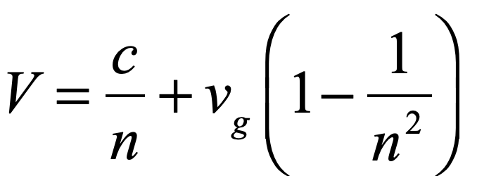
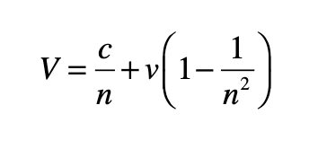
Fresnel realized that Arago’s null results could be explained if aether was only partially dragged along by matter. For instance, in the glass prisms used by Arago, the fraction of the aether being dragged along by the moving glass versus at rest would depend on the refractive index n of the glass. The speed of light in moving glass would then be
where c is the speed of light through stationary aether, vg is the speed of the glass prism through the stationary aether, and V is the speed of light in the moving glass. The first term in the expression is the ordinary definition of the speed of light in stationary matter with the refractive index. The second term is called the Fresnel drag coefficient which he communicated to Arago in a letter in 1818. Even at the high speed of the Earth moving around the sun, this second term is a correction of only about one part in ten thousand. It explained Arago’s null results for stellar aberration, but it was not possible to measure it directly in the laboratory at that time.
Fizeau’s Moving Water Experiment
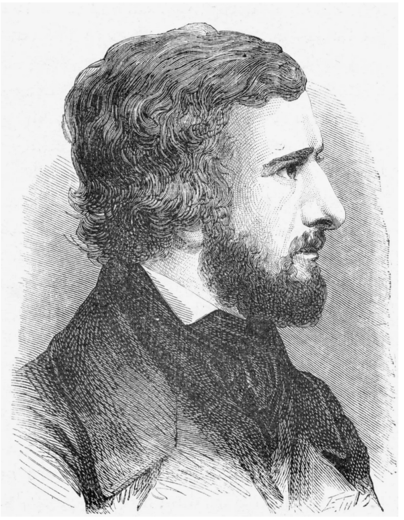
Hippolyte Fizeau has the distinction of being the first to measure the speed of light directly in an Earth-bound experiment. All previous measurements had been astronomical. The story of his ingenious use of a chopper wheel and long-distance reflecting mirrors placed across the city of Paris in 1849 can be found in Chapter 3 of Interference. However, two years later he completed an experiment that few at the time noticed but which had a much more profound impact on the history of physics.
Hippolyte Fizeau
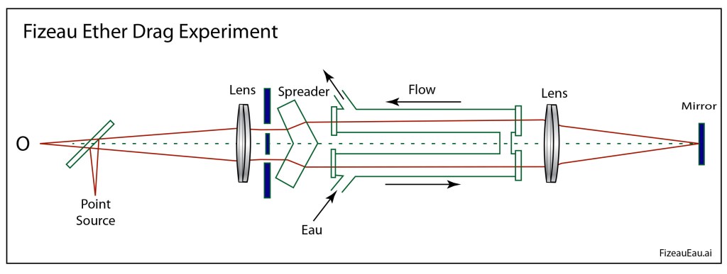
In 1851, Fizeau modified an Arago interferometer to pass two interfering light beams along pipes of moving water. The goal of the experiment was to measure the aether drag coefficient directly and to test Fresnel’s theory of partial aether drag. The interferometer allowed Fizeau to measure the speed of light in moving water relative to the speed of light in stationary water. The results of the experiment confirmed Fresnel’s drag coefficient to high accuracy, which seemed to confirm the partial drag of aether by moving matter.
Fizeau’s 1851 measurement of the speed of light in water using a modified Arago interferometer. (Reprinted from Chapter 2: Interference.)
This result stood for thirty years, presenting its own challenges for physicist exploring theories of the aether. The sophistication of interferometry improved over that time, and in 1881 Albert Michelson used his newly-invented interferometer to measure the speed of the Earth through the aether. He performed the experiment in the Potsdam Observatory outside Berlin, Germany, and found the opposite result of complete aether drag, contradicting Fizeau’s experiment. Later, after he began collaborating with Edwin Morley at Case and Western Reserve Colleges in Cleveland, Ohio, the two repeated Fizeau’s experiment to even better precision, finding once again Fresnel’s drag coefficient, followed by their own experiment, known now as “the Michelson-Morley Experiment” in 1887, that found no effect of the Earth’s movement through the aether.
The two experiments—Fizeau’s measurement of the Fresnel drag coefficient, and Michelson’s null measurement of the Earth’s motion—were in direct contradiction with each other. Based on the theory of the aether, they could not both be true.
But where to go from there? For the next 15 years, there were numerous attempts to put bandages on the aether theory, from Fitzgerald’s contraction to Lorenz’ transformations, but it all seemed like kludges built on top of kludges. None of it was elegant—until Einstein had his crucial insight.
Einstein’s Insight
While all the other top physicists at the time were trying to save the aether, taking its real existence as a fact of Nature to be reconciled with experiment, Einstein took the opposite approach—he assumed that the aether did not exist and began looking for what the experimental consequences would be.
From the days of Galileo, it was known that measured speeds depended on the frame of reference. This is why a knife dropped by a sailor climbing the mast of a moving ship strikes at the base of the mast, falling in a straight line in the sailor’s frame of reference, but an observer on the shore sees the knife making an arc—velocities of relative motion must add. But physicists had over-generalized this result and tried to apply it to light—Arago, Fresnel, Fizeau, Michelson, Lorenz—they were all locked in a mindset.
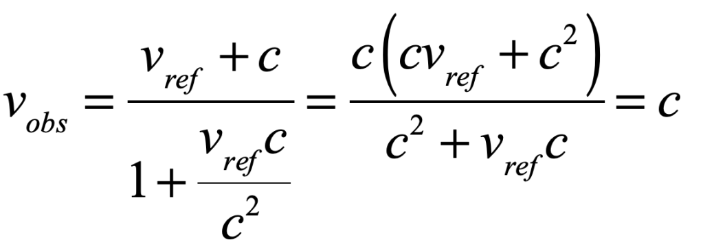
Einstein stepped outside that mindset and asked what would happen if all relatively moving observers measured the same value for the speed of light, regardless of their relative motion. It was just a little algebra to find that the way to add the speed of light c to the speed of a moving reference frame vref was
where the numerator was the usual Galilean relativity velocity addition, and the denominator was required to enforce the constancy of observed light speeds. Therefore, adding the speed of light to the speed of a moving reference frame gives back simply the speed of light.
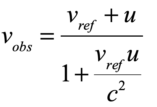
Generalizing this equation for general velocity addition between moving frames gives
where u is now the speed of some moving object being added the the speed of a reference frame, and vobs is the “net” speed observed by some “external” observer . This is Einstein’s famous equation for relativistic velocity addition (see pg. 12 of the English translation). It ensures that all observers with differently moving frames all measure the same speed of light, while also predicting that no velocities for objects can ever exceed the speed of light.
This last fact is a consequence, not an assumption, as can be seen by letting the reference speed vref increase towards the speed of light so that vref ≈ c, then
so that the speed of an object launched in the forward direction from a reference frame moving near the speed of light is still observed to be no faster than the speed of light
All of this, so far, is theoretical. Einstein then looked to find some experimental verification of his new theory of relativistic velocity addition, and he thought of the Fizeau experimental measurement of the speed of light in moving water. Applying his new velocity addition formula to the Fizeau experiment, he set vref = vwater and u = c/n and found
The second term in the denominator is much smaller that unity and is expanded in a Taylor’s expansion
The last line is exactly the Fresnel drag coefficient!
Therefore, Fizeau, half a century before, in 1851, had already provided experimental verification of Einstein’s new theory for relativistic velocity addition! It wasn’t aether drag at all—it was relativistic velocity addition.
From this point onward, Einstein followed consequence after inexorable consequence, constructing what is now called his theory of Special Relativity, complete with relativistic transformations of time and space and energy and matter—all following from a simple postulate of the constancy of the speed of light and the prescription for the addition of velocities.
The final irony is that Einstein used Fresnel’s theoretical coefficient and Fizeau’s measurements, that had established aether drag in the first place, as the proof he needed to show that there was no aether. It was all just how you looked at it.
• The history behind Einstein’s use of relativistic velocity addition is given in: A. Pais, Subtle is the Lord: The Science and the Life of Albert Einstein (Oxford University Press, 2005).
Despite the many apparent paradoxes posed in physics—the twin and ladder paradoxes of relativity theory, Olber’s paradox of the bright night sky, Loschmitt’s paradox of irreversible statistical fluctuations—these are resolved by a deeper look at the underlying assumptions—the twin paradox is resolved by considering shifts in reference frames, the ladder paradox is resolved by the loss of simultaneity, Olber’s paradox is resolved by a finite age to the universe, and Loschmitt’s paradox is resolved by fluctuation theorems. In each case, no physical principle is violated, and each paradox is fully explained.
However, there is at least one “true” paradox in physics that defies consistent explanation—quantum entanglement. Quantum entanglement was first described by Einstein with colleagues Podolsky and Rosen in the famous EPR paper of 1935 as an argument against the completeness of quantum mechanics, and it was given its name by Schrödinger the same year in the paper where he introduced his “cat” as a burlesque consequence of entanglement.
Here is a short history of quantum entanglement [1], from its beginnings in 1935 to the recent 2022 Nobel prize in Physics awarded to John Clauser, Alain Aspect and Anton Zeilinger.
The EPR Papers of 1935
Einstein can be considered as the father of quantum mechanics, even over Planck, because of his 1905 derivation of the existence of the photon as a discrete carrier of a quantum of energy (see Einstein versus Planck). Even so, as Heisenberg and Bohr advanced quantum mechanics in the mid 1920’s, emphasizing the underlying non-deterministic outcomes of measurements, and in particular the notion of instantaneous wavefunction collapse, they pushed the theory in directions that Einstein found increasingly disturbing and unacceptable.
This feature is an excerpt from an upcoming book, Interference: The History of Optical Interferometry and the Scientists Who Tamed Light (Oxford University Press, July 2023), by David D. Nolte.
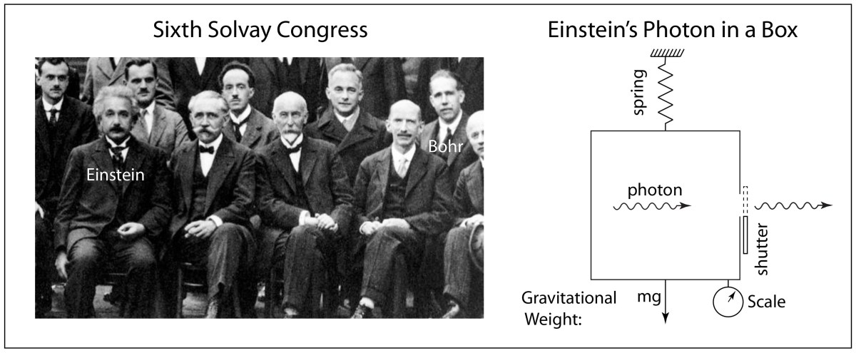
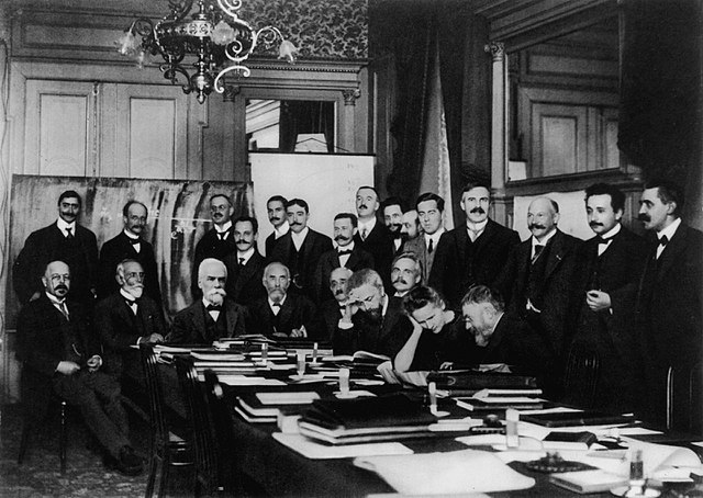
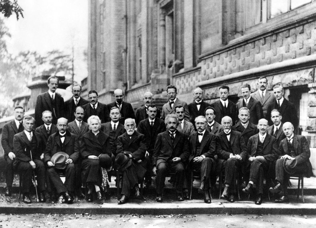
At the invitation-only Solvay Congresses of 1927 and 1930, where all the top physicists met to debate the latest advances, Einstein and Bohr began a running debate that was epic in the history of physics as the two top minds went head-to-head as the onlookers looked on in awe. Ultimately, Einstein was on the losing end. Although he was convinced that something was missing in quantum theory, he could not counter all of Bohr’s rejoinders, even as Einstein’s assaults became ever more sophisticated, and he left the field of battle beaten but not convinced. Several years later he launched his last and ultimate salvo.
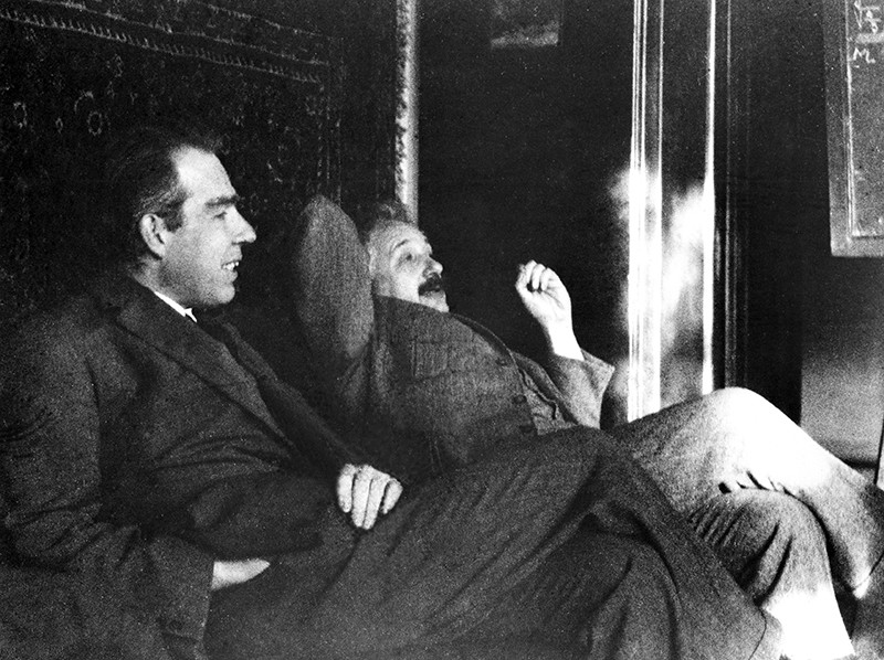
Fig. 1 Niels Bohr and Albert Einstein
At the Institute for Advanced Study in Princeton, New Jersey, in the 1930’s Einstein was working with Nathan Rosen and Boris Podolsky when he envisioned a fundamental paradox in quantum theory that occurred when two widely-separated quantum particles were required to share specific physical properties because of simple conservation theorems like energy and momentum. Even Bohr and Heisenberg could not deny the principle of conservation of energy and momentum, and Einstein devised a two-particle system for which these conservation principles led to an apparent violation of Heisenberg’s own uncertainty principle. He left the details to his colleagues, with Podolsky writing up the main arguments. They published the paper in the Physical Review in March of 1935 with the title “Can Quantum-Mechanical Description of Physical Reality be Considered Complete” [2]. Because of the three names on the paper (Einstein, Podolsky, Rosen), it became known as the EPR paper, and the paradox they presented became known as the EPR paradox.
When Bohr read the paper, he was initially stumped and aghast. He felt that EPR had shaken the very foundations of the quantum theory that he and his institute had fought so hard to establish. He also suspected that EPR had made a mistake in their arguments, and he halted all work at his institute in Copenhagen until they could construct a definitive answer. A few months later, Bohr published a paper in the Physical Review in July of 1935, using the identical title that EPR had used, in which he refuted the EPR paradox [3]. There is not a single equation or figure in the paper, but he used his “awful incantation terminology” to maximum effect, showing that one of the EPR assumptions on the assessment of uncertainties to position and momentum was in error, and he was right.
Einstein was disgusted. He had hoped that this ultimate argument against the completeness of quantum mechanics would stand the test of time, but Bohr had shot it down within mere months. Einstein was particularly disappointed with Podolsky, because Podolsky had tried too hard to make the argument specific to position and momentum, leaving a loophole for Bohr to wiggle through, where Einstein had wanted the argument to rest on deeper and more general principles.
Despite Bohr’s victory, Einstein had been correct in his initial formulation of the EPR paradox that showed quantum mechanics did not jibe with common notions of reality. He and Schrödinger exchanged letters commiserating with each other and encouraging each other in their counter beliefs against Bohr and Heisenberg. In November of 1935, Schrödinger published a broad, mostly philosophical, paper in Naturwissenschaften [4] in which he amplified the EPR paradox with the use of an absurd—what he called burlesque—consequence of wavefunction collapse that became known as Schrödinger’s Cat. He also gave the central property of the EPR paradox its name: entanglement.
Ironically, both Einstein’s entanglement paradox and Schrödinger’s Cat, which were formulated originally to be arguments against the validity of quantum theory, have become established quantum tools. Today, entangled particles are the core workhorses of quantum information systems, and physicists are building larger and larger versions of Schrödinger’s Cat that may eventually merge with the physics of the macroscopic world.
Bohm and Ahronov Tackle EPR
The physicist David Bohm was a rare political exile from the United States. He was born in the heart of Pennsylvania in the town of Wilkes-Barre, attended Penn State and then the University of California at Berkeley, where he joined Robert Oppenheimer’s research group. While there, he became deeply involved in the fight for unions and socialism, activities for which he was called before McCarthy’s Committee on Un-American Activities. He invoked his right to the fifth amendment for which he was arrested. Although he was later acquitted, Princeton University fired him from his faculty position, and fearing another arrest, he fled to Brazil where his US passport was confiscated by American authorities. He had become a physicist without a country.
Fig. 2 David Bohm
Despite his personal trials, Bohm remained scientifically productive. He published his influential textbook on quantum mechanics in the midst of his Senate hearings, and after a particularly stimulating discussion with Einstein shortly before he fled the US, he developed and published an alternative version of quantum theory in 1952 that was fully deterministic—removing Einstein’s “God playing dice”—by creating a hidden-variable theory [5].
Hidden-variable theories of quantum mechanics seek to remove the randomness of quantum measurement by assuming that some deeper element of quantum phenomena—a hidden variable—explains each outcome. But it is also assumed that these hidden variables are not directly accessible to experiment. In this sense, the quantum theory of Bohr and Heisenberg was “correct” but not “complete”, because there were things that the theory could not predict or explain.
Bohm’s hidden variable theory, based on a quantum potential, was able to reproduce all the known results of standard quantum theory without invoking the random experimental outcomes that Einstein abhorred. However, it still contained one crucial element that could not sweep away the EPR paradox—it was nonlocal.
Nonlocality lies at the heart of quantum theory. In its simplest form, the nonlocal nature of quantum phenomenon says that quantum states span spacetime with space-like separations, meaning that parts of the wavefunction are non-causally connected to other parts of the wavefunction. Because Einstein was fundamentally committed to causality, the nonlocality of quantum theory was what he found most objectionable, and Bohm’s elegant hidden-variable theory, that removed Einstein’s dreaded randomness, could not remove that last objection of non-causality.
After working in Brazil for several years, Bohm moved to the Technion University in Israel where he began a fruitful collaboration with Yakir Ahronov. In addition to proposing the Ahronov-Bohm effect, in 1957 they reformulated Podolsky’s version of the EPR paradox that relied on continuous values of position and momentum and replaced it with a much simpler model based on the Stern-Gerlach effect on spins and further to the case of positronium decay into two photons with correlated polarizations. Bohm and Ahronov reassessed experimental results of positronium decay that had been made by Madame Wu in 1950 at Columbia University and found it in full agreement with standard quantum theory.
John Bell’s Inequalities
John Stuart Bell had an unusual start for a physicist. His family was too poor to give him an education appropriate to his skills, so he enrolled in vocational school where he took practical classes that included brick laying. Working later as a technician in a university lab, he caught the attention of his professors who sponsored him to attend the university. With a degree in physics, he began working at CERN as an accelerator designer when he again caught the attention of his supervisors who sponsored him to attend graduate school. He graduated with a PhD and returned to CERN as a card-carrying physicist with all the rights and privileges that entailed.
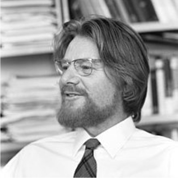
Fig. 3 John Bell
During his university days, he had been fascinated by the EPR paradox, and he continued thinking about the fundamentals of quantum theory. On a sabbatical to the Stanford accelerator in 1960 he began putting mathematics to the EPR paradox to see whether any local hidden variable theory could be compatible with quantum mechanics. His analysis was fully general, so that it could rule out as-yet-unthought-of hidden-variable theories. The result of this work was a set of inequalities that must be obeyed by any local hidden-variable theory. Then he made a simple check using the known results of quantum measurement and showed that his inequalities are violated by quantum systems. This ruled out the possibility of any local hidden variable theory (but not Bohm’s nonlocal hidden-variable theory). Bell published his analysis in 1964 [6] in an obscure journal that almost no one read…except for a curious graduate student at Columbia University who began digging into the fundamental underpinnings of quantum theory against his supervisor’s advice.
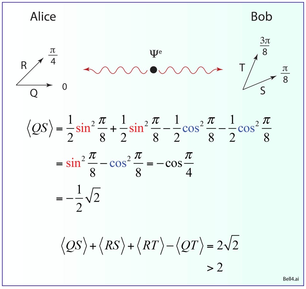
Fig. 4 Polarization measurements on entangled photons violate Bell’s inequality.
John Clauser’s Tenacious Pursuit
As a graduate student in astrophysics at Columbia University, John Clauser was supposed to be doing astrophysics. Instead, he spent his time musing over the fundamentals of quantum theory. In 1967 Clauser stumbled across Bell’s paper while he was in the library. The paper caught his imagination, but he also recognized that the inequalities were not experimentally testable, because they required measurements that depended directly on hidden variables, which are not accessible. He began thinking of ways to construct similar inequalities that could be put to an experimental test, and he wrote about his ideas to Bell, who responded with encouragement. Clauser wrote up his ideas in an abstract for an upcoming meeting of the American Physical Society, where one of the abstract reviewers was Abner Shimony of Boston University. Clauser was surprised weeks later when he received a telephone call from Shimony. Shimony and his graduate student Micheal Horne had been thinking along similar lines, and Shimony proposed to Clauser that they join forces. They met in Boston where they were met Richard Holt, a graudate student at Harvard who was working on experimental tests of quantum mechanics. Collectively, they devised a new type of Bell inequality that could be put to experimental test [7]. The result has become known as the CHSH Bell inequality (after Clauser, Horne, Shimony and Holt).
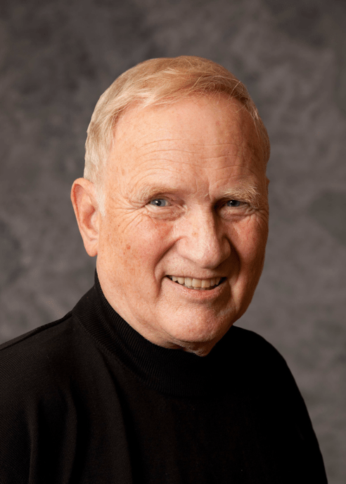
Fig. 5 John Clauser
When Clauser took a post-doc position in Berkeley, he began searching for a way to do the experiments to test the CHSH inequality, even though Holt had a head start at Harvard. Clauser enlisted the help of Charles Townes, who convinced one of the Berkeley faculty to loan Clauser his graduate student, Stuart Freedman, to help. Clauser and Freedman performed the experiments, using a two-photon optical decay of calcium ions and found a violation of the CHSH inequality by 5 standard deviations, publishing their result in 1972 [8].
Fig. 6 CHSH inequality violated by entangled photons.
Alain Aspect’s Non-locality
Just as Clauser’s life was changed when he stumbled on Bell’s obscure paper in 1967, the paper had the same effect on the life of French physicist Alain Aspect who stumbled on it in 1975. Like Clauser, he also sought out Bell for his opinion, meeting with him in Geneva, and Aspect similarly received Bell’s encouragement, this time with the hope to build upon Clauser’s work.
Fig. 7 Alain Aspect
In some respects, the conceptual breakthrough achieved by Clauser had been the CHSH inequality that could be tested experimentally. The subsequent Clauser Freedman experiments were not a conclusion, but were just the beginning, opening the door to deeper tests. For instance, in the Clauser-Freedman experiments, the polarizers were static, and the detectors were not widely separated, which allowed the measurements to be time-like separated in spacetime. Therefore, the fundamental non-local nature of quantum physics had not been tested.
Aspect began a thorough and systematic program, that would take him nearly a decade to complete, to test the CHSH inequality under conditions of non-locality. He began with a much brighter source of photons produced using laser excitation of the calcium ions. This allowed him to perform the experiment in 100’s of seconds instead of the hundreds of hours by Clauser. With such a high data rate, Aspect was able to verify violation of the Bell inequality to 10 standard deviations, published in 1981 [9].
However, the real goal was to change the orientations of the polarizers while the photons were in flight to widely separated detectors [10]. This experiment would allow the detection to be space-like separated in spacetime. The experiments were performed using fast-switching acoustic-optic modulators, and the Bell inequality was violated to 5 standard deviations [11]. This was the most stringent test yet performed and the first to fully demonstrate the non-local nature of quantum physics.
Anton Zeilinger: Master of Entanglement
If there is one physicist today whose work encompasses the broadest range of entangled phenomena, it would be the Austrian physicist, Anton Zeilinger. He began his career in neutron interferometery, but when he was bitten by the entanglement bug in 1976, he switched to quantum photonics because of the superior control that can be exercised using optics over sources and receivers and all the optical manipulations in between.
Fig. 8 Anton Zeilinger
Working with Daniel Greenberger and Micheal Horne, they took the essential next step past the Bohm two-particle entanglement to consider a 3-particle entangled state that had surprising properties. While the violation of locality by the two-particle entanglement was observed through the statistical properties of many measurements, the new 3-particle entanglement could show violations on single measurements, further strengthening the arguments for quantum non-locality. This new state is called the GHZ state (after Greenberger, Horne and Zeilinger) [12].
As the Zeilinger group in Vienna was working towards experimental demonstrations of the GHZ state, Charles Bennett of IBM proposed the possibility for quantum teleportation, using entanglement as a core quantum information resource [13]. Zeilinger realized that his experimental set-up could perform an experimental demonstration of the effect, and in a rapid re-tooling of the experimental apparatus [14], the Zeilinger group was the first to demonstrate quantum teleportation that satisfied the conditions of the Bennett teleportation proposal [15]. An Italian-UK collaboration also made an early demonstration of a related form of teleportation in a paper that was submitted first, but published after Zeilinger’s, due to delays in review [16]. But teleportation was just one of a widening array of quantum applications for entanglement that was pursued by the Zeilinger group over the succeeding 30 years [17], including entanglement swapping, quantum repeaters, and entanglement-based quantum cryptography. Perhaps most striking, he has worked on projects at astronomical observatories that entangle photons coming from cosmic sources.
By David D. Nolte Nov. 26, 2022
Read more about the history of quantum entanglement in Interference (New From Oxford University Press, 2023)
A popular account of the trials and toils of the scientists and engineers who tamed light and used it to probe the universe.
[2] A. Einstein, B. Podolsky, N. Rosen, Can quantum-mechanical description of physical reality be considered complete? Physical Review47, 0777-0780 (1935).
[3] N. Bohr, Can quantum-mechanical description of physical reality be considered complete? Physical Review48, 696-702 (1935).
[4] E. Schrödinger, Die gegenwärtige Situation in der Quantenmechanik. Die Naturwissenschaften 23, 807-12; 823-28; 844-49 (1935).
[5] D. Bohm, A suggested interpretation of the quantum theory in terms of hidden variables .1. Physical Review85, 166-179 (1952); D. Bohm, A suggested interpretation of the quantum theory in terms of hidden variables .2. Physical Review85, 180-193 (1952).
[6] J. Bell, On the Einstein-Podolsky-Rosen paradox. Physics1, 195 (1964).
[7] 1. J. F. Clauser, M. A. Horne, A. Shimony, R. A. Holt, Proposed experiment to test local hidden-variable theories. Physical Review Letters23, 880-& (1969).
[8] S. J. Freedman, J. F. Clauser, Experimental test of local hidden-variable theories. Physical Review Letters28, 938-& (1972).
[9] A. Aspect, P. Grangier, G. Roger, EXPERIMENTAL TESTS OF REALISTIC LOCAL THEORIES VIA BELLS THEOREM. Physical Review Letters47, 460-463 (1981).
[10] Alain Aspect, Bell’s Theorem: The Naïve Veiw of an Experimentalit. (2004), hal- 00001079
[11] A. Aspect, J. Dalibard, G. Roger, EXPERIMENTAL TEST OF BELL INEQUALITIES USING TIME-VARYING ANALYZERS. Physical Review Letters49, 1804-1807 (1982).
[12] D. M. Greenberger, M. A. Horne, A. Zeilinger, in 1988 Fall Workshop on Bells Theorem, Quantum Theory and Conceptions of the Universe. (George Mason Univ, Fairfax, Va, 1988), vol. 37, pp. 69-72.
[13] C. H. Bennett, G. Brassard, C. Crepeau, R. Jozsa, A. Peres, W. K. Wootters, Teleporting an unknown quantum state via dual classical and einstein-podolsky-rosen channels. Physical Review Letters70, 1895-1899 (1993).
[14] J. Gea-Banacloche, Optical realizations of quantum teleportation, in Progress in Optics, Vol 46, E. Wolf, Ed. (2004), vol. 46, pp. 311-353.
[15] D. Bouwmeester, J.-W. Pan, K. Mattle, M. Eibl, H. Weinfurter, A. Zeilinger, Experimental quantum teleportation. Nature390, 575-579 (1997).
[16] D. Boschi, S. Branca, F. De Martini, L. Hardy, S. Popescu, Experimental realization of teleporting an unknown pure quantum state via dual classical and Einstein-podolsky-Rosen Channels. Phys. Rev. Lett.80, 1121-1125 (1998).
[17] A. Zeilinger, Light for the quantum. Entangled photons and their applications: a very personal perspective. Physica Scripta92, 1-33 (2017).
One of the hardest aspects to grasp about relativity theory is the question of whether an event “looks as if” it is doing something, or whether it “actually is” doing something.
Take, for instance, the classic twin paradox of relativity theory in which there are twins who wear identical high-precision wrist watches. One of them rockets off to Alpha Centauri at relativistic speeds and returns while the other twin stays on Earth. Each twin sees the other twin’s clock running slowly because of relativistic time dilation. Yet when they get back together and, standing side-by-side, they compare their watches—the twin who went to Alpha Centauri is actually younger than the other, despite the paradox. The relativistic effect of time dilation is “real”, not just apparent, regardless of whether they come back together to do the comparison.
Yet this understanding of relativistic effects took many years, even decades, to gain acceptance after Einstein proposed them. He was aware himself that key experiments were required to prove that relativistic effects are real and not just apparent.
Einstein and the Transverse Doppler Effect
In 1905 Einstein used his new theory of special relativity to predict observable consequences that included relativistic velocity addition and a general treatment of the relativistic Doppler effect [1]. This included the effects of time dilation in addition to the longitudinal effect of the source chasing the wave. Time dilation produced a correction to Doppler’s original expression for the longitudinal effect that became significant at speeds approaching the speed of light. More significantly, it predicted a transverse Doppler effect for a source moving along a line perpendicular to the line of sight to an observer. This effect had not been predicted either by Christian Doppler (1803 – 1853) or by Woldemar Voigt (1850 – 1919).
Despite the generally positive reception of Einstein’s theory of special relativity, some of its consequences were anathema to many physicists at the time. A key stumbling block was the question whether relativistic effects, like moving clocks running slowly, were only apparent, or were actually real, and Einstein had to fight to convince others of its reality. When Johannes Stark (1874 – 1957) observed Doppler line shifts in ion beams called “canal rays” in 1906 (Stark received the 1919 Nobel prize in part for this discovery) [3], Einstein promptly published a paper suggesting how the canal rays could be used in a transverse geometry to directly detect time dilation through the transverse Doppler effect [4]. Thirty years passed before the experiment was performed with sufficient accuracy by Herbert Ives and G. R. Stilwell in 1938 to measure the transverse Doppler effect [5]. Ironically, even at this late date, Ives and Stilwell were convinced that their experiment had disproved Einstein’s time dilation by supporting Lorentz’ contraction theory of the electron. The Ives-Stilwell experiment was the first direct test of time dilation, followed in 1940 by muon lifetime measurements [6].
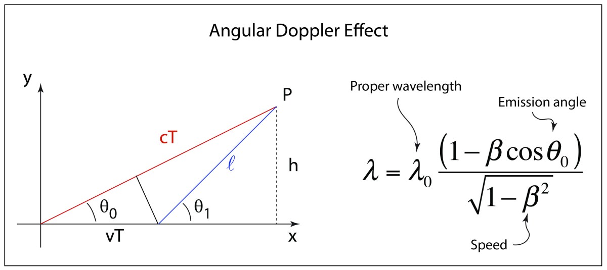
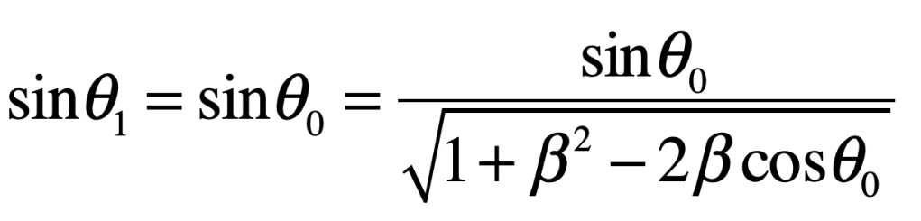
A) Transverse Doppler Shift Relative to EmissionAngle
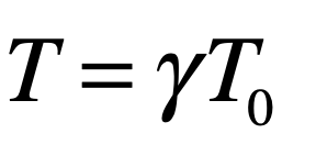
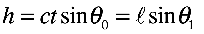
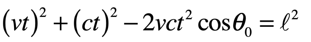
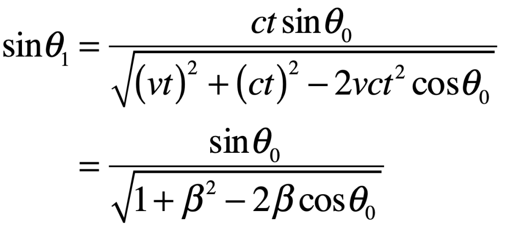
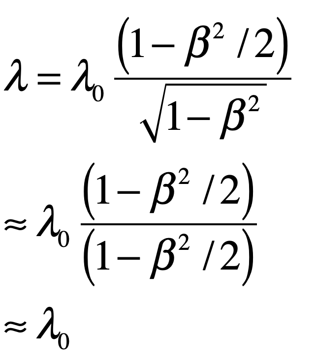
The Doppler effect varies between blue shifts in the forward direction to red shifts in the backward direction, with a smooth variation in Doppler shift as a function of the emission angle. Consider the configuration shown in Fig. 1 for light emitted from a source moving at speed v and emitting at an angle θ0 in the receiver frame. The source moves a distance vT in the time of a single emission cycle (assume a harmonic wave). In that time T (which is the period of oscillation of the light source — or the period of a clock if we think of it putting out light pulses) the light travels a distance cT before another cycle begins (or another pulse is emitted).
Fig. 1 Configuration for detection of Doppler shifts for emission angle θ0. The light source travels a distance vT during the time of a single cycle, while the wavefront travels a distance cT towards the detector.
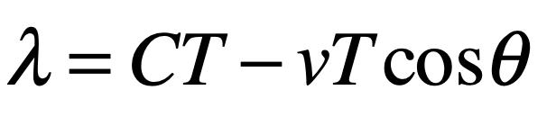
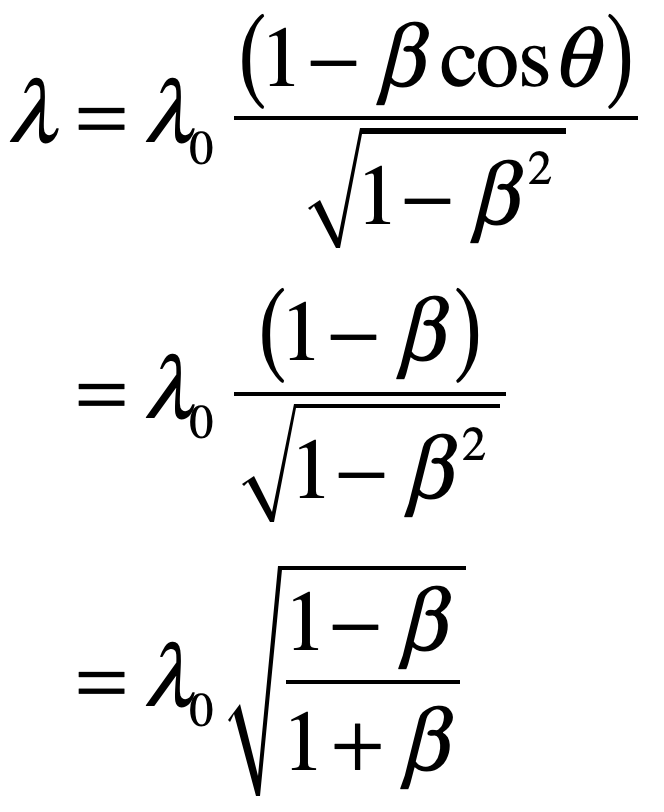
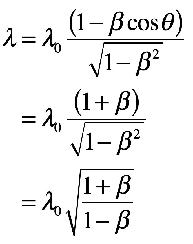
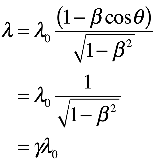
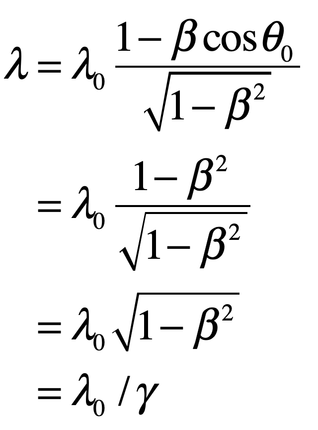
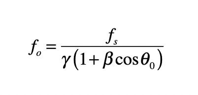
The observed wavelength in the receiver frame is thus given by
where T is the emission period of the moving source. Importantly, the emission period is time dilated relative to the proper emission time of the source
Therefore,
This expression can be evaluated for several special cases:
a) θ0 = 0 for forward emission
which is the relativistic blue shift for longitudinal motion in the direction of the receiver.
b) θ0 = π for backward emission
which is the relativistic red shift for longitudinal motion away from the receiver
c) θ0 = π/2 for transverse emission
This transverse Doppler effect for emission at right angles is a red shift, caused only by the time dilation of the moving light source. This is the effect proposed by Einstein and observed by Stark that proved moving clocks tick slowly. But it is not the only way to view the transverse Doppler effect.
B) Transverse Doppler Shift Relative to Angle at Reception
A different option for viewing the transverse Doppler effect is the angle to the moving source at the moment that the light is detected. The geometry of this configuration relative to the previous is illustrated in Fig. 2.
Fig. 2 The detection point is drawn at a finite distance. However, the relationship between θ0 and θ1 is independent of the distance to the detector
The transverse distance to the detection point is
The length of the line connecting the detection point P with the location of the light source at the moment of detection is (using the law of cosines)
Combining with the first equation gives
An equivalent expression is obtained as
Note that this result, relating θ1 to θ0, is independent of the distance to the observation point.
When θ1 = π/2, then
yielding
for which the Doppler effect is
which is a blue shift. This creates the unexpected result that sin θ0 = π/2 produces a red shift, while sin θ1 = π/2 produces a blue shift. The question could be asked: which one represents time dilation? In fact, it is sin θ0 = π/2 that produces time dilation exclusively, because in that configuration there is no foreshortening effect on the wavelength–only the emission time.
C) Compromise: The Null Transverse Doppler Shift
The previous two configurations each could be used as a definition for the transverse Doppler effect. But one gives a red shift and one gives a blue shift, which seems contradictory. Therefore, one might try to strike a compromise between these two cases so that sin θ1 = sin θ0, and the configuration is shown in Fig. 3.
This is the case when θ1 + θ2 = π. The sines of the two angles are equal, yielding
and
which is solved for
Inserting this into the Doppler equation gives
where the Taylor’s expansion of the denominator (at low speed) cancels the numerator to give zero net Doppler shift. This compromise configuration represents the condition of null Doppler frequency shift. However, for speeds approaching the speed of light, the net effect is a lengthening of the wavelength, dominated by time dilation, causing a red shift.
D) Source in Circular Motion Around Receiver
An interesting twist can be added to the problem of the transverse Doppler effect: put the source or receiver into circular motion, one about the other. In the case of a source in circular motion around the receiver, it is easy to see that this looks just like case A) above for θ0 = π/2, which is the red shift caused by the time dilation of the moving source
However, there is the possible complication that the source is no longer in an inertial frame (it experiences angular acceleration) and therefore it is in the realm of general relativity instead of special relativity. In fact, it was Einstein’s solution to this problem that led him to propose the Equivalence Principle and make his first calculations on the deflection of light by gravity. His solution was to think of an infinite number of inertial frames, each of which was instantaneously co-moving with the same linear velocity as the source. These co-moving frames are inertial and can be analyzed using the principles of special relativity. The general relativistic effects come from slipping from one inertial co-moving frame to the next. But in the case of the circular transverse Doppler effect, each instantaneously co-moving frame has the exact configuration as case A) above, and so the wavelength is red shifted exactly by the time dilation.
Fig. Left: Moving source around a stationary receiver has red-shifted light (pure time dilation effect). Right. Moving receiver around a stationary source has blue-shifted light.
E) Receiver in Circular Motion Around Source
Now flip the situation and consider a moving receiver orbiting a stationary source.
With the notion of co-moving inertial frames now in hand, this configuration is exactly the same as case B) above, and the wavelength is blue shifted according to the equation
caused by foreshortening.
By David D. Nolte, June 3, 2021
New from Oxford Press: The History of Light and Interference (2023)
Read about the physics and history of light and optics.
[3] J. Stark, W. Hermann, and S. Kinoshita, “The Doppler effect in the spectrum of mercury,” Annalen Der Physik, vol. 21, pp. 462-469, Nov 1906.
[4] A. Einstein, “Possibility of a new examination of the relativity principle,” Annalen Der Physik, vol. 23, no. 6, pp. 197-198, May (1907)
[5] H. E. Ives and G. R. Stilwell, “An experimental study of the rate of a moving atomic clock,” Journal of the Optical Society of America, vol. 28, p. 215, 1938.
[6] B. Rossi and D. B. Hall, “Variation of the Rate of Decay of Mesotrons with Momentum,” Physical Review, vol. 59, pp. 223–228, 1941.
“Society is founded on hero worship”, wrote Thomas Carlyle (1795 – 1881) in his 1840 lecture on “Hero as Divinity”—and the society of physicists is no different. Among physicists, the hero is the genius—the monomyth who journeys into the supernatural realm of high mathematics, engages in single combat against chaos and confusion, gains enlightenment in the mysteries of the universe, and returns home to share the new understanding. If the hero is endowed with unusual talent and achieves greatness, then mythologies are woven, creating shadows that can grow and eclipse the truth and the work of others, bestowing upon the hero recognitions that are not entirely deserved.
“Gentlemen! The views of space and time which I wish to lay before you … They are radical. Henceforth space by itself, and time by itself, are doomed to fade away into mere shadows, and only a kind of union of the two will preserve an independent reality.”
Herman Minkowski (1908)
The greatest hero of physics of the twentieth century, without question, is Albert Einstein. He is the person most responsible for the development of “Modern Physics” that encompasses:
Relativity theory (both special and general),
Quantum theory (he invented the quantum in 1905—see my blog),
Astrophysics (his field equations of general relativity were solved by Schwarzschild in 1916 to predict event horizons of black holes, and he solved his own equations to predict gravitational waves that were discovered in 2015),
Cosmology (his cosmological constant is now recognized as the mysterious dark energy that was discovered in 2000), and
Solid state physics (his explanation of the specific heat of crystals inaugurated the field of quantum matter).
Einstein made so many seminal contributions to so many sub-fields of physics that it defies comprehension—hence he is mythologized as genius, able to see into the depths of reality with unique insight. He deserves his reputation as the greatest physicist of the twentieth century—he has my vote, and he was chosen by Time magazine in 2000 as the Man of the Century. But as his shadow has grown, it has eclipsed and even assimilated the work of others—work that he initially criticized and dismissed, yet later embraced so whole-heartedly that he is mistakenly given credit for its discovery.
For instance, when we think of Einstein, the first thing that pops into our minds is probably “spacetime”. He himself wrote several popular accounts of relativity that incorporated the view that spacetime is the natural geometry within which so many of the non-intuitive properties of relativity can be understood. When we think of time being mixed with space, making it seem that position coordinates and time coordinates share an equal place in the description of relativistic physics, it is common to attribute this understanding to Einstein. Yet Einstein initially resisted this viewpoint and even disparaged it when he first heard it!
Spacetime was the brain-child of Hermann Minkowski.
Minkowski in Königsberg
Hermann Minkowski was born in 1864 in Russia to German parents who moved to the city of Königsberg (King’s Mountain) in East Prussia when he was eight years old. He entered the university in Königsberg in 1880 when he was sixteen. Within a year, when he was only seventeen years old, and while he was still a student at the University, Minkowski responded to an announcement of the Mathematics Prize of the French Academy of Sciences in 1881. When he submitted is prize-winning memoire, he could have had no idea that it was starting him down a path that would lead him years later to revolutionary views.
A view of Königsberg in 1581. Six of the seven bridges of Königsberg—which Euler famously described in the first essay on topology—are seen in this picture. The University is in the center distance behind the castle. The city was destroyed by the Russians in WWII followed by a forced evacuation of the local population.
The specific Prize challenge of 1881 was to find the number of representations of an integer as a sum of five squares of integers. For instance, every integer n > 33 can be expressed as the sum of five nonzero squares. As an example, 42 = 22 + 22 + 32 + 32 + 42, which is the only representation for that number. However, there are five representation for n = 53
The task of enumerating these representations draws from the theory of quadratic forms. A quadratic form is a function of products of numbers with integer coefficients, such as ax2 + bxy + cy2 and ax2 + by2 + cz2 + dxy + exz + fyz. In number theory, one seeks to find integer solutions for which the quadratic form equals an integer. For instance, the Pythagorean theorem x2 + y2 = n2 for integers is a quadratic form for which there are many integer solutions (x,y,n), known as Pythagorean triplets, such as
The topic of quadratic forms gained special significance after the work of Bernhard Riemann who established the properties of metric spaces based on the metric expression
for infinitesimal distance in a D-dimensional metric space. This is a generalization of Euclidean distance to more general non-Euclidean spaces that may have curvature. Minkowski would later use this expression to great advantage, developing a “Geometry of Numbers” [1] as he delved ever deeper into quadratic forms and their uses in number theory.
Minkowski in Göttingen
After graduating with a doctoral degree in 1885 from Königsberg, Minkowski did his habilitation at the university of Bonn and began teaching, moving back to Königsberg in 1892 and then to Zurich in 1894 (where one of his students was a somewhat lazy and unimpressive Albert Einstein). A few years later he was given an offer that he could not refuse.
At the turn of the 20th century, the place to be in mathematics was at the University of Göttingen. It had a long tradition of mathematical giants that included Carl Friedrich Gauss, Bernhard Riemann, Peter Dirichlet, and Felix Klein. Under the guidance of Felix Klein, Göttingen mathematics had undergone a renaissance. For instance, Klein had attracted Hilbert from the University of Königsberg in 1895. David Hilbert had known Minkowski when they were both students in Königsberg, and Hilbert extended an invitation to Minkowski to join him in Göttingen, which Minkowski accepted in 1902.
The University of Göttingen
A few years after Minkowski arrived at Göttingen, the relativity revolution broke, and both Minkowski and Hilbert began working on mathematical aspects of the new physics. They organized a colloquium dedicated to relativity and related topics, and on Nov. 5, 1907 Minkowski gave his first tentative address on the geometry of relativity.
Because Minkowski’s specialty was quadratic forms, and given his understanding of Riemann’s work, he was perfectly situated to apply his theory of quadratic forms and invariants to the Lorentz transformations derived by Poincaré and Einstein. Although Poincaré had published a paper in 1906 that showed that the Lorentz transformation was a generalized rotation in four-dimensional space [2], Poincaré continued to discuss space and time as separate phenomena, as did Einstein. For them, simultaneity was no longer an invariant, but events in time were still events in time and not somehow mixed with space-like properties. Minkowski recognized that Poincaré had missed an opportunity to define a four-dimensional vector space filled by four-vectors that captured all possible events in a single coordinate description without the need to separate out time and space.
Minkowski’s first attempt, presented in his 1907 colloquium, at constructing velocity four-vectors was flawed because (like so many of my mechanics students when they first take a time derivative of the four-position) he had not yet understood the correct use of proper time. But the research program he outlined paved the way for the great work that was to follow.
On Feb. 21, 1908, only 3 months after his first halting steps, Minkowski delivered a thick manuscript to the printers for an article to appear in the Göttinger Nachrichten. The title “Die Grundgleichungen für die elektromagnetischen Vorgänge in bewegten Körpern” (The Basic Equations for Electromagnetic Processes of Moving Bodies) belies the impact and importance of this very dense article [3]. In its 60 pages (with no figures), Minkowski presents the correct form for four-velocity by taking derivatives relative to proper time, and he formalizes his four-dimensional approach to relativity that became the standard afterwards. He introduces the terms spacelikevector, timelike vector, light cone and world line. He also presents the complete four-tensor form for the electromagnetic fields. The foundational work of Levi Cevita and Ricci-Curbastro on tensors was not yet well known, so Minkowski invents his own terminology of Traktor to describe it. Most importantly, he invents the terms spacetime (Raum-Zeit) and events (Erignisse) [4].
Minkowski’s four-dimensional formalism of relativistic electromagnetics was more than a mathematical trick—it uncovered the presence of a multitude of invariants that were obscured by the conventional mathematics of Einstein and Lorentz and Poincaré. In Minkowski’s approach, whenever a proper four-vector is contracted with itself (its inner product), an invariant emerges. Because there are many fundamental four-vectors, there are many invariants. These invariants provide the anchors from which to understand the complex relative properties amongst relatively moving frames.
Minkowski’s master work appeared in the Nachrichten on April 5, 1908. If he had thought that physicists would embrace his visionary perspective, he was about to be woefully disabused of that notion.
Einstein’s Reaction
Despite his impressive ability to see into the foundational depths of the physical world, Einstein did not view mathematics as the root of reality. Mathematics for him was a tool to reduce physical intuition into quantitative form. In 1908 his fame was rising as the acknowledged leader in relativistic physics, and he was not impressed or pleased with the abstract mathematical form that Minkowski was trying to stuff the physics into. Einstein called it “superfluous erudition” [5], and complained “since the mathematics pounced on the relativity theory, I no longer understand it myself! [6]”
With his collaborator Jakob Laub (also a former student of Minkowski’s), Einstein objected to more than the hard-to-follow mathematics—they believed that Minkowski’s form of the pondermotive force was incorrect. They then proceeded to re-translate Minkowski’s elegant four-vector derivations back into ordinary vector analysis, publishing two papers in Annalen der Physik in the summer of 1908 that were politely critical of Minkowski’s approach [7-8]. Yet another of Minkowski’s students from Zurich, Gunnar Nordström, showed how to derive Minkowski’s field equations without any of the four-vector formalism.
One can only wonder why so many of his former students so easily dismissed Minkowski’s revolutionary work. Einstein had actually avoided Minkowski’s mathematics classes as a student at ETH [5], which may say something about Minkowski’s reputation among the students, although Einstein did appreciate the class on mechanics that he took from Minkowski. Nonetheless, Einstein missed the point! Rather than realizing the power and universality of the four-dimensional spacetime formulation, he dismissed it as obscure and irrelevant—perhaps prejudiced by his earlier dim view of his former teacher.
Raum und Zeit
It is clear that Minkowski was stung by the poor reception of his spacetime theory. It is also clear that he truly believed that he had uncovered an essential new approach to physical reality. While mathematicians were generally receptive of his work, he knew that if physicists were to adopt his new viewpoint, he needed to win them over with the elegant results.
In 1908, Minkowski presented a now-famous paper Raum und Zeit at the 80thAssembly of German Natural Scientists and Physicians (21 September 1908). In his opening address, he stated [9]:
“Gentlemen! The views of space and time which I wish to lay before you have sprung from the soil of experimental physics, and therein lies their strength. They are radical. Henceforth space by itself, and time by itself, are doomed to fade away into mere shadows, and only a kind of union of the two will preserve an independent reality.”
To illustrate his arguments Minkowski constructed the most recognizable visual icon of relativity theory—the space-time diagram in which the trajectories of particles appear as “world lines”, as in Fig. 1. On this diagram, one spatial dimension is plotted along the horizontal-axis, and the value ct (speed of light times time) is plotted along the vertical-axis. In these units, a photon travels along a line oriented at 45 degrees, and the world-line (the name Minkowski gave to trajectories) of all massive particles must have slopes steeper than this. For instance, a stationary particle, that appears to have no trajectory at all, executes a vertical trajectory on the space-time diagram as it travels forward through time. Within this new formulation by Minkowski, space and time were mixed together in a single manifold—spacetime—and were no longer separate entities.
Fig. 1 The First “Minkowski diagram” of spacetime.
In addition to the spacetime construct, Minkowski’s great discovery was the plethora of invariants that followed from his geometry. For instance, the spacetime hyperbola
is invariant to Lorentz transformation in coordinates. This is just a simple statement that a vector is an entity of reality that is independent of how it is described. The length of a vector in our normal three-space does not change if we flip the coordinates around or rotate them, and the same is true for four-vectors in Minkowski space subject to Lorentz transformations.
In relativity theory, this property of invariance becomes especially useful because part of the mental challenge of relativity is that everything looks different when viewed from different frames. How do you get a good grip on a phenomenon if it is always changing, always relative to one frame or another? The invariants become the anchors that we can hold on to as reference frames shift and morph about us.
Fig. 2 Any event on an invariant hyperbola is transformed by the Lorentz transformation onto another point on the same hyperbola. Events that are simultaneous in one frame are each on a separate hyperbola. After transformation, simultaneity is lost, but each event stays on its own invariant hyperbola (Figure reprinted from [10]).
As an example of a fundamental invariant, the mass of a particle in its rest frame becomes an invariant mass, always with the same value. In earlier relativity theory, even in Einstein’s papers, the mass of an object was a function of its speed. How is the mass of an electron a fundamental property of physics if it is a function of how fast it is traveling? The construction of invariant mass removes this problem, and the mass of the electron becomes an immutable property of physics, independent of the frame. Invariant mass is just one of many invariants that emerge from Minkowski’s space-time description. The study of relativity, where all things seem relative, became a study of invariants, where many things never change. In this sense, the theory of relativity is a misnomer. Ironically, relativity theory became the motivation of post-modern relativism that denies the existence of absolutes, even as relativity theory, as practiced by physicists, is all about absolutes.
Despite his audacious gambit to win over the physicists, Minkowski would not live to see the fruits of his effort. He died suddenly of a burst gall bladder on Jan. 12, 1909 at the age of 44.
Arnold Sommerfeld (who went on to play a central role in the development of quantum theory) took up Minkowski’s four vectors, and he systematized it in a way that was palatable to physicists. Then Max von Laue extended it while he was working with Sommerfeld in Munich, publishing the first physics textbook on relativity theory in 1911, establishing the space-time formalism for future generations of German physicists. Further support for Minkowski’s work came from his distinguished colleagues at Göttingen (Hilbert, Klein, Wiechert, Schwarzschild) as well as his former students (Born, Laue, Kaluza, Frank, Noether). With such champions, Minkowski’s work was immortalized in the methodology (and mythology) of physics, representing one of the crowning achievements of the Göttingen mathematical community.
Einstein Relents
Already in 1907 Einstein was beginning to grapple with the role of gravity in the context of relativity theory, and he knew that the special theory was just a beginning. Yet between 1908 and 1910 Einstein’s focus was on the quantum of light as he defended and extended his unique view of the photon and prepared for the first Solvay Congress of 1911. As he returned his attention to the problem of gravitation after 1910, he began to realize that Minkowski’s formalism provided a framework from which to understand the role of accelerating frames. In 1912 Einstein wrote to Sommerfeld to say [5]
I occupy myself now exclusively with the problem of gravitation . One thing is certain that I have never before had to toil anywhere near as much, and that I have been infused with great respect for mathematics, which I had up until now in my naivety looked upon as a pure luxury in its more subtle parts. Compared to this problem. the original theory of relativity is child’s play.
By the time Einstein had finished his general theory of relativity and gravitation in 1915, he fully acknowledge his indebtedness to Minkowski’s spacetime formalism without which his general theory may never have appeared.
By David D. Nolte, April 24, 2021
[1] H. Minkowski, Geometrie der Zahlen. Leipzig and Berlin: R. G. Teubner, 1910.
[4] S. Walter, “Minkowski’s Modern World,” in Minkowski Spacetime: A Hundred Years Later, Petkov Ed.: Springer, 2010, ch. 2, pp. 43-61.
[5] L. Corry, “The influence of David Hilbert and Hermann Minkowski on Einstein’s views over the interrelation between physics and mathematics,” Endeavour, vol. 22, no. 3, pp. 95-97, (1998)
[6] A. Pais, Subtle is the Lord: The Science and the Life of Albert Einstein. Oxford, 2005.
[7] A. Einstein and J. Laub, “Electromagnetic basic equations for moving bodies,” Annalen Der Physik, vol. 26, no. 8, pp. 532-540, Jul (1908)
[8] A. Einstein and J. Laub, “Electromagnetic fields on quiet bodies with pondermotive energy,” Annalen Der Physik, vol. 26, no. 8, pp. 541-550, Jul (1908)
[9] Minkowski, H. (1909). “Raum und Zeit.” Jahresbericht der Deutschen Mathematikier-Vereinigung: 75-88.
Einstein is the alpha of the quantum. Einstein is also the omega. Although he was the one who established the quantum of energy and matter (see my Blog Einstein vs Planck), Einstein pitted himself in a running debate against Niels Bohr’s emerging interpretation of quantum physics that had, in Einstein’s opinion, severe deficiencies. Between sessions during a series of conferences known as the Solvay Congresses over a period of eight years from 1927 to 1935, Einstein constructed a challenges of increasing sophistication to confront Bohr and his quasi-voodoo attitudes about wave-function collapse. To meet the challenge, Bohr sharpened his arguments and bested Einstein, who ultimately withdrew from the field of battle. Einstein, as quantum physics’ harshest critic, played a pivotal role, almost against his will, establishing the Copenhagen interpretation of quantum physics that rules to this day, and also inventing the principle of entanglement which lies at the core of almost all quantum information technology today.
Debate Timeline
Fifth Solvay Congress: 1927 October Brussels: Debate Round 1
Einstein and ensembles
Sixth Solvay Congress: 1930 Debate Round 2
Photon in a box
Seventh Solvay Congress: 1933
Einstein absent (visiting the US when Hitler takes power…decides not to return to Germany.)
Physical Review 1935: Debate Round 3
EPR paper and Bohr’s response
Schrödinger’s Cat
Notable Nobel Prizes
1918 Planck
1921 Einstein
1922 Bohr
1932 Heisenberg
1933 Dirac and Schrödinger
The Solvay Conferences
The Solvay congresses were unparalleled scientific meetings of their day. They were attended by invitation only, and invitations were offered only to the top physicists concerned with the selected topic of each meeting. The Solvay congresses were held about every three years always in Belgium, supported by the Belgian chemical industrialist Ernest Solvay. The first meeting, held in 1911, was on the topic of radiation and quanta.
Fig. 1 First Solvay Congress (1911). Einstein (standing second from right) was one of the youngest attendees.
The fifth meeting, held in 1927, was on electrons and photons and focused on the recent rapid advances in quantum theory. The old quantum guard was invited—Planck, Bohr and Einstein. The new quantum guard was invited as well—Heisenberg, de Broglie, Schrödinger, Born, Pauli, and Dirac. Heisenberg and Bohr joined forces to present a united front meant to solidify what later became known as the Copenhagen interpretation of quantum physics. The basic principles of the interpretation include the wavefunction of Schrödinger, the probabilistic interpretation of Born, the uncertainty principle of Heisenberg, the complementarity principle of Bohr and the collapse of the wavefunction during measurement. The chief conclusion that Heisenberg and Bohr sought to impress on the assembled attendees was that the theory of quantum processes was complete, meaning that unknown or uncertain characteristics of measurements could not be attributed to lack of knowledge or understanding, but were fundamental and permanently inaccessible.
Fig. 2 Fifth Solvay Congress (1927). Einstein front and center. Bohr on the far right middle row.
Einstein was not convinced with that argument, and he rose to his feet to object after Bohr’s informal presentation of his complementarity principle. Einstein insisted that uncertainties in measurement were not fundamental, but were caused by incomplete information, that , if known, would accurately account for the measurement results. Bohr was not prepared for Einstein’s critique and brushed it off, but what ensued in the dining hall and the hallways of the Hotel Metropole in Brussels over the next several days has become one of the most famous scientific debates of the modern era, known as the Bohr-Einstein debate on the meaning of quantum theory. The debate gently raged night and day through the fifth congress, and was renewed three years later at the 1930 congress. It finished, in a final flurry of published papers in 1935 that launched some of the central concepts of quantum theory, including the idea of quantum entanglement and, of course, Schrödinger’s cat.
Einstein’s strategy, to refute Bohr, was to construct careful thought experiments that envisioned perfect experiments, without errors, that measured properties of ideal quantum systems. His aim was to paint Bohr into a corner from which he could not escape, caught by what Einstein assumed was the inconsistency of complementarity. Einstein’s “thought experiments” used electrons passing through slits, diffracting as required by Schrödinger’s theory, but being detected by classical measurements. Einstein would present a thought experiment to Bohr, who would then retreat to consider the way around Einstein’s arguments, returning the next hour or the next day with his answer, only to be confronted by yet another clever device of Einstein’s clever imagination that would force Bohr to retreat again. The spirit of this back and forth encounter between Bohr and Einstein is caught dramatically in the words of Paul Ehrenfest who witnessed the debate first hand, partially mediating between Bohr and Einstein, both of whom he respected deeply.
“Brussels-Solvay was fine!… BOHR towering over everybody. At first not understood at all … , then step by step defeating everybody. Naturally, once again the awful Bohr incantation terminology. Impossible for anyone else to summarise … (Every night at 1 a.m., Bohr came into my room just to say ONE SINGLE WORD to me, until three a.m.) It was delightful for me to be present during the conversation between Bohr and Einstein. Like a game of chess, Einstein all the time with new examples. In a certain sense a sort of Perpetuum Mobile of the second kind to break the UNCERTAINTY RELATION. Bohr from out of philosophical smoke clouds constantly searching for the tools to crush one example after the other. Einstein like a jack-in-the-box; jumping out fresh every morning. Oh, that was priceless. But I am almost without reservation pro Bohr and contra Einstein. His attitude to Bohr is now exacly like the attitude of the defenders of absolute simultaneity towards him …” [1]
The most difficult example that Einstein constructed during the fifth Solvary Congress involved an electron double-slit apparatus that could measure, in principle, the momentum imparted to the slit by the passing electron, as shown in Fig.3. The electron gun is a point source that emits the electrons in a range of angles that illuminates the two slits. The slits are small relative to a de Broglie wavelength, so the electron wavefunctions diffract according to Schrödinger’s wave mechanics to illuminate the detection plate. Because of the interference of the electron waves from the two slits, electrons are detected clustered in intense fringes separated by dark fringes.
So far, everyone was in agreement with these suggested results. The key next step is the assumption that the electron gun emits only a single electron at a time, so that only one electron is present in the system at any given time. Furthermore, the screen with the double slit is suspended on a spring, and the position of the screen is measured with complete accuracy by a displacement meter. When the single electron passes through the entire system, it imparts a momentum kick to the screen, which is measured by the meter. It is also detected at a specific location on the detection plate. Knowing the position of the electron detection, and the momentum kick to the screen, provides information about which slit the electron passed through, and gives simultaneous position and momentum values to the electron that have no uncertainty, apparently rebutting the uncertainty principle.
Fig. 3 Einstein’s single-electron thought experiment in which the recoil of the screen holding the slits can be measured to tell which way the electron went. Bohr showed that the more “which way” information is obtained, the more washed-out the interference pattern becomes.
This challenge by Einstein was the culmination of successively more sophisticated examples that he had to pose to combat Bohr, and Bohr was not going to let it pass unanswered. With ingenious insight, Bohr recognized that the key element in the apparatus was the fact that the screen with the slits must have finite mass if the momentum kick by the electron were to produce a measurable displacement. But if the screen has finite mass, and hence a finite momentum kick from the electron, then there must be an uncertainty in the position of the slits. This uncertainty immediately translates into a washout of the interference fringes. In fact the more information that is obtained about which slit the electron passed through, the more the interference is washed out. It was a perfect example of Bohr’s own complementarity principle. The more the apparatus measures particle properties, the less it measures wave properties, and vice versa, in a perfect balance between waves and particles.
Einstein grudgingly admitted defeat at the end of the first round, but he was not defeated. Three years later he came back armed with more clever thought experiments, ready for the second round in the debate.
The Sixth Solvay Conference: 1930
At the Solvay Congress of 1930, Einstein was ready with even more difficult challenges. His ultimate idea was to construct a box containing photons, just like the original black bodies that launched Planck’s quantum hypothesis thirty years before. The box is attached to a weighing scale so that the weight of the box plus the photons inside can be measured with arbitrarily accuracy. A shutter over a hole in the box is opened for a time T, and a photon is emitted. Because the photon has energy, it has an equivalent weight (Einstein’s own famous E = mc2), and the mass of the box changes by an amount equal to the photon energy divided by the speed of light squared: m = E/c2. If the scale has arbitrary accuracy, then the energy of the photon has no uncertainty. In addition, because the shutter was open for only a time T, the time of emission similarly has no uncertainty. Therefore, the product of the energy uncertainty and the time uncertainty is much smaller than Planck’s constant, apparently violating Heisenberg’s precious uncertainty principle.
Bohr was stopped in his tracks with this challenge. Although he sensed immediately that Einstein had missed something (because Bohr had complete confidence in the uncertainty principle), he could not put his finger immediately on what it was. That evening he wandered from one attendee to another, very unhappy, trying to persuade them and saying that Einstein could not be right because it would be the end of physics. At the end of the evening, Bohr was no closer to a solution, and Einstein was looking smug. However, by the next morning Bohr reappeared tired but in high spirits, and he delivered a master stroke. Where Einstein had used special relaitivity against Bohr, Bohr now used Einstein’s own general relativity against him.
The key insight was that the weight of the box must be measured, and the process of measurement was just as important as the quantum process being measured—this was one of the cornerstones of the Copenhagen interpretation. So Bohr envisioned a measuring apparatus composed of a spring and a scale with the box suspended in gravity from the spring. As the photon leaves the box, the weight of the box changes, and so does the deflection of the spring, changing the height of the box. This change in height, in a gravitational potential, causes the timing of the shutter to change according to the law of gravitational time dilation in general relativity. By calculating the the general relativistic uncertainty in the time, coupled with the special relativistic uncertainty in the weight of the box, produced a product that was at least as big as Planck’s constant—Heisenberg’s uncertainty principle was saved!
Fig. 4 Einstein’s thought experiment that uses special relativity to refute quantum mechanics. Bohr then invoked Einstein’s own general relativity to refute him.
Entanglement and Schrödinger’s Cat
Einstein ceded the point to Bohr but was not convinced. He still believed that quantum mechanics was not a “complete” theory of quantum physics and he continued to search for the perfect thought experiment that Bohr could not escape. Even today when we have become so familiar with quantum phenomena, the Copenhagen interpretation of quantum mechanics has weird consequences that seem to defy common sense, so it is understandable that Einstein had his reservations.
After the sixth Solvay congress Einstein and Schrödinger exchanged many letters complaining to each other about Bohr’s increasing strangle-hold on the interpretation of quantum mechanics. Egging each other on, they both constructed their own final assault on Bohr. The irony is that the concepts they devised to throw down quantum mechanics have today become cornerstones of the theory. For Einstein, his final salvo was “Entanglement”. For Schrödinger, his final salvo was his “cat”. Today, Entanglement and Schrödinger’s Cat have become enshrined on the alter of quantum interpretation even though their original function was to thwart that interpretation.
The final round of the debate was carried out, not at a Solvay congress, but in the Physical review journal by Einstein [2] and Bohr [3], and in the Naturwissenshaften by Schrödinger [4].
In 1969, Heisenberg looked back on these years and said,
To those of us who participated in the development of atomic theory, the five years following the Solvay Conference in Brussels in 1927 looked so wonderful that we often spoke of them as the golden age of atomic physics. The great obstacles that had occupied all our efforts in the preceding years had been cleared out of the way, the gate to an entirely new field, the quantum mechanics of the atomic shells stood wide open, and fresh fruits seemed ready for the picking. [5]
The Physics of Life, the Universe and Everything:
Read more about the history of modern dynamics in Galileo Unbound from Oxford University Press
[1] A. Whitaker, Einstein, Bohr, and the quantum dilemma : from quantum theory to quantum information, 2nd ed. Cambridge University Press, 2006. (pg. 210)
[2] A. Einstein, B. Podolsky, and N. Rosen, “Can quantum-mechanical description of physical reality be considered complete?,” Physical Review, vol. 47, no. 10, pp. 0777-0780, May (1935)
[3] N. Bohr, “Can quantum-mechanical description of physical reality be considered complete?,” Physical Review, vol. 48, no. 8, pp. 696-702, Oct (1935)
Christian Andreas Doppler (1803 – 1853) was born in Salzburg, Austria, to a longstanding family of stonemasons. As a second son, he was expected to help his older brother run the business, so his Father had him tested in his 18th year for his suitability for a career in business. The examiner Simon Stampfer (1790 – 1864), an Austrian mathematician and inventor teaching at the Lyceum in Salzburg, discovered that Doppler had a gift for mathematics and was better suited for a scientific career. Stampfer’s enthusiasm convinced Doppler’s father to enroll him in the Polytechnik Institute in Vienna (founded only a few years earlier in 1815) where he took classes in mathematics, mechanics and physics [1] from 1822 to 1825. Doppler excelled in his courses, but was dissatisfied with the narrowness of the education, yearning for more breadth and depth in his studies and for more significance in his positions, feelings he would struggle with for his entire short life. He left Vienna, returning to the Lyceum in Salzburg to round out his education with philosophy, languages and poetry. Unfortunately, this four-year detour away from technical studies impeded his ability to gain a permanent technical position, so he began a temporary assistantship with a mathematics professor at Vienna. As he approached his 30th birthday this term expired without prospects. He was about to emigrate to America when he finally received an offer to teach at a secondary school in Prague.
To read about the attack by Joseph Petzval on Doppler’s effect and the effect it had on Doppler, see my feature article “The Fall and Rise of the Doppler Effect“ in Physics Today, 73(3) 30, March (2020).
Salzburg Austria
Doppler in Prague
Prague gave Doppler new life. He was a professor with a position that allowed him to marry the daughter of a sliver and goldsmith from Salzburg. He began to publish scholarly papers, and in 1837 was appointed supplementary professor of Higher Mathematics and Geometry at the Prague Technical Institute, promoted to full professor in 1841. It was here that he met the unusual genius Bernard Bolzano (1781 – 1848), recently returned from political exile in the countryside. Bolzano was a philosopher and mathematician who developed rigorous concepts of mathematical limits and is famous today for his part in the Bolzano-Weierstrass theorem in functional analysis, but he had been too liberal and too outspoken for the conservative Austrian regime and had been dismissed from the University in Prague in 1819. He was forbidden to publish his work in Austrian journals, which is one reason why much of Bolzano’s groundbreaking work in functional analysis remained unknown during his lifetime. However, he participated in the Bohemian Society for Science from a distance, recognizing the inventive tendencies in the newcomer Doppler and supporting him for membership in the Bohemian Society. When Bolzano was allowed to return in 1842 to the Polytechnic Institute in Prague, he and Doppler became close friends as kindred spirits.
Prague, Czech Republic
On May 25, 1842, Bolzano presided as chairman over a meeting of the Bohemian Society for Science on the day that Doppler read a landmark paper on the color of stars to a meagre assembly of only five regular members of the Society [2]. The turn-out was so small that the meeting may have been held in the robing room of the Society rather than in the meeting hall itself. Leading up to this famous moment, Doppler’s interests were peripatetic, ranging widely over mathematical and physical topics, but he had lately become fascinated by astronomy and by the phenomenon of stellar aberration. Stellar aberration was discovered by James Bradley in 1729 and explained as the result of the Earth’s yearly motion around the Sun, causing the apparent location of a distant star to change slightly depending on the direction of the Earth’s motion. Bradley explained this in terms of the finite speed of light and was able to estimate it to within several percent [3]. As Doppler studied Bradley aberration, he wondered how the relative motion of the Earth would affect the color of the star. By making a simple analogy of a ship traveling with, or against, a series of ocean waves, he concluded that the frequency of impact of the peaks and troughs of waves on the ship was no different than the arrival of peaks and troughs of the light waves impinging on the eye. Because perceived color was related to the frequency of excitation in the eye, he concluded that the color of light would be slightly shifted to the blue if approaching, and to the red if receding from, the light source.
Doppler wave fronts from a source emitting spherical waves moving with speeds β relative to the speed of the wave in the medium.
Doppler calculated the magnitude of the effect by taking a simple ratio of the speed of the observer relative to the speed of light. What he found was that the speed of the Earth, though sufficient to cause the detectable aberration in the position of stars, was insufficient to produce a noticeable change in color. However, his interest in astronomy had made him familiar with binary stars where the relative motion of the light source might be high enough to cause color shifts. In fact, in the star catalogs there were examples of binary stars that had complementary red and blue colors. Therefore, the title of his paper, published in the Proceedings of the Royal Bohemian Society of Sciences a few months after he read it to the society, was “On the Coloured Light of the Double Stars and Certain Other Stars of the Heavens: Attempt at a General Theory which Incorporates Bradley’s Theorem of Aberration as an Integral Part” [4].
Title page of Doppler’s 1842 paper introducing the Doppler Effect.
Doppler’s analogy was correct, but like all analogies not founded on physical law, it differed in detail from the true nature of the phenomenon. By 1842 the transverse character of light waves had been thoroughly proven through the work of Fresnel and Arago several decades earlier, yet Doppler held onto the old-fashioned notion that light was composed of longitudinal waves. Bolzano, fully versed in the transverse nature of light, kindly published a commentary shortly afterwards [5] showing how the transverse effect for light, and a longitudinal effect for sound, were both supported by Doppler’s idea. Yet Doppler also did not know that speeds in visual binaries were too small to produce noticeable color effects to the unaided eye. Finally, (and perhaps the greatest flaw in his argument on the color of stars) a continuous spectrum that extends from the visible into the infrared and ultraviolet would not change color because all the frequencies would shift together preserving the flat (white) spectrum.
The simple algebraic derivation of the Doppler Effect in the 1842 publication..
Doppler’s twelve years in Prague were intense. He was consumed by his Society responsibilities and by an extremely heavy teaching load that included personal exams of hundreds of students. The only time he could be creative was during the night while his wife and children slept. Overworked and running on too little rest, his health already frail with the onset of tuberculosis, Doppler collapsed, and he was unable to continue at the Polytechnic. In 1847 he transferred to the School of Mines and Forrestry in Schemnitz (modern Banská Štiavnica in Slovakia) with more pay and less work. Yet the revolutions of 1848 swept across Europe, with student uprisings, barricades in the streets, and Hungarian liberation armies occupying the cities and universities, giving him no peace. Providentially, his former mentor Stampfer retired from the Polytechnic in Vienna, and Doppler was called to fill the vacancy.
Although Doppler was named the Director of Austria’s first Institute of Physics and was elected to the National Academy, he ran afoul of one of the other Academy members, Joseph Petzval (1807 – 1891), who persecuted Doppler and his effect. To read a detailed description of the attack by Petzval on Doppler’s effect and the effect it had on Doppler, see my feature article “The Fall and Rise of the Doppler Effect” in Physics Today, March issue (2020).
Christian Doppler
Voigt’s Transformation
It is difficult today to appreciate just how deeply engrained the reality of the luminiferous ether was in the psyche of the 19th century physicist. The last of the classical physicists were reluctant even to adopt Maxwell’s electromagnetic theory for the explanation of optical phenomena, and as physicists inevitably were compelled to do so, some of their colleagues looked on with dismay and disappointment. This was the situation for Woldemar Voigt (1850 – 1919) at the University of Göttingen, who was appointed as one of the first professors of physics there in 1883, to be succeeded in later years by Peter Debye and Max Born. Voigt received his doctorate at the University of Königsberg under Franz Neumann, exploring the elastic properties of rock salt, and at Göttingen he spent a quarter century pursuing experimental and theoretical research into crystalline properties. Voigt’s research, with students like Paul Drude, laid the foundation for the modern field of solid state physics. His textbook Lehrbuch der Kristallphysik published in 1910 remained influential well into the 20th century because it adopted mathematical symmetry as a guiding principle of physics. It was in the context of his studies of crystal elasticity that he introduced the word “tensor” into the language of physics.
At the January 1887 meeting of the Royal Society of Science at Göttingen, three months before Michelson and Morely began their reality-altering experiments at the Case Western Reserve University in Cleveland Ohio, Voit submitted a paper deriving the longitudinal optical Doppler effect in an incompressible medium. He was responding to results published in 1886 by Michelson and Morely on their measurements of the Fresnel drag coefficient, which was the precursor to their later results on the absolute motion of the Earth through the ether.
Fresnel drag is the effect of light propagating through a medium that is in motion. The French physicist Francois Arago (1786 – 1853) in 1810 had attempted to observe the effects of corpuscles of light emitted from stars propagating with different speeds through the ether as the Earth spun on its axis and traveled around the sun. He succeeded only in observing ordinary stellar aberration. The absence of the effects of motion through the ether motivated Augustin-Jean Fresnel (1788 – 1827) to apply his newly-developed wave theory of light to explain the null results. In 1818 Fresnel derived an expression for the dragging of light by a moving medium that explained the absence of effects in Arago’s observations. For light propagating through a medium of refractive index n that is moving at a speed v, the resultant velocity of light is
where the last term in parenthesis is the Fresnel drag coefficient. The Fresnel drag effect supported the idea of the ether by explaining why its effects could not be observed—a kind of Catch-22—but it also applied to light moving through a moving dielectric medium. In 1851, Fizeau used an interferometer to measure the Fresnel drag coefficient for light moving through moving water, arriving at conclusions that directly confirmed the Fresnel drag effect. The positive experiments of Fizeau, as well as the phenomenon of stellar aberration, would be extremely influential on the thoughts of Einstein as he developed his approach to special relativity in 1905. They were also extremely influential to Michelson, Morley and Voigt.
In his paper on the absence of the Fresnel drag effect in the first Michelson-Morley experiment, Voigt pointed out that an equation of the form
is invariant under the transformation
From our modern vantage point, we immediately recognize (to within a scale factor) the Lorentz transformation of relativity theory. The first equation is common Galilean relativity, but the last equation was something new, introducing a position-dependent time as an observer moved with speed relative to the speed of light [6]. Using these equations, Voigt was the first to derive the longitudinal (conventional) Doppler effect from relativistic effects.
Voigt’s derivation of the longitudinal Doppler effect used a classical approach that is still used today in Modern Physics textbooks to derive the Doppler effect. The argument proceeds by considering a moving source that emits a continuous wave in the direction of motion. Because the wave propagates at a finite speed, the moving source chases the leading edge of the wave front, catching up by a small amount by the time a single cycle of the wave has been emitted. The resulting compressed oscillation represents a blue shift of the emitted light. By using his transformations, Voigt arrived at the first relativistic expression for the shift in light frequency. At low speeds, Voigt’s derivation reverted to Doppler’s original expression.
A few months after Voigt delivered his paper, Michelson and Morley announced the results of their interferometric measurements of the motion of the Earth through the ether—with their null results. In retrospect, the Michelson-Morley experiment is viewed as one of the monumental assaults on the old classical physics, helping to launch the relativity revolution. However, in its own day, it was little more than just another null result on the ether. It did incite Fitzgerald and Lorentz to suggest that length of the arms of the interferometer contracted in the direction of motion, with the eventual emergence of the full Lorentz transformations by 1904—seventeen years after the Michelson results.
In 1904 Einstein, working in relative isolation at the Swiss patent office, was surprisingly unaware of the latest advances in the physics of the ether. He did not know about Voigt’s derivation of the relativistic Doppler effect (1887) as he had not heard of Lorentz’s final version of relativistic coordinate transformations (1904). His thinking about relativistic effects focused much farther into the past, to Bradley’s stellar aberration (1725) and Fizeau’s experiment of light propagating through moving water (1851). Einstein proceeded on simple principles, unencumbered by the mental baggage of the day, and delivered his beautifully minimalist theory of special relativity in his famous paper of 1905 “On the Electrodynamics of Moving Bodies”, independently deriving the Lorentz coordinate transformations [7].
One of Einstein’s talents in theoretical physics was to predict new phenomena as a way to provide direct confirmation of a new theory. This was how he later famously predicted the deflection of light by the Sun and the gravitational frequency shift of light. In 1905 he used his new theory of special relativity to predict observable consequences that included a general treatment of the relativistic Doppler effect. This included the effects of time dilation in addition to the longitudinal effect of the source chasing the wave. Time dilation produced a correction to Doppler’s original expression for the longitudinal effect that became significant at speeds approaching the speed of light. More significantly, it predicted a transverse Doppler effect for a source moving along a line perpendicular to the line of sight to an observer. This effect had not been predicted either by Doppler or by Voigt. The equation for the general Doppler effect for any observation angle is
Just as Doppler had been motivated by Bradley’s aberration of starlight when he conceived of his original principle for the longitudinal Doppler effect, Einstein combined the general Doppler effect with his results for the relativistic addition of velocities (also in his 1905 Annalen paper) as the conclusive treatment of stellar aberration nearly 200 years after Bradley first observed the effect.
Despite the generally positive reception of Einstein’s theory of special relativity, some of its consequences were anathema to many physicists at the time. A key stumbling block was the question whether relativistic effects, like moving clocks running slowly, were only apparent, or were actually real, and Einstein had to fight to convince others of its reality. When Johannes Stark (1874 – 1957) observed Doppler line shifts in ion beams called “canal rays” in 1906 (Stark received the 1919 Nobel prize in part for this discovery) [8], Einstein promptly published a paper suggesting how the canal rays could be used in a transverse geometry to directly detect time dilation through the transverse Doppler effect [9]. Thirty years passed before the experiment was performed with sufficient accuracy by Herbert Ives and G. R. Stilwell in 1938 to measure the transverse Doppler effect [10]. Ironically, even at this late date, Ives and Stilwell were convinced that their experiment had disproved Einstein’s time dilation by supporting Lorentz’ contraction theory of the electron. The Ives-Stilwell experiment was the first direct test of time dilation, followed in 1940 by muon lifetime measurements [11].
[3] Bradley, J (1729). “Account of a new discoved Motion of the Fix’d Stars”. Phil Trans. 35: 637–660.
[4] C. A. DOPPLER, “Über das farbige Licht der Doppelsterne und einiger anderer Gestirne des Himmels (About the coloured light of the binary stars and some other stars of the heavens),” Proceedings of the Royal Bohemian Society of Sciences, vol. V, no. 2, pp. 465–482, (Reissued 1903) (1842).
[5] B. Bolzano, “Ein Paar Bemerkunen über die Neu Theorie in Herrn Professor Ch. Doppler’s Schrift “Über das farbige Licht der Doppersterne und eineger anderer Gestirnedes Himmels”,” Pogg. Anal. der Physik und Chemie, vol. 60, p. 83, 1843; B. Bolzano, “Christian Doppler’s neuste Leistunen af dem Gebiet der physikalischen Apparatenlehre, Akoustik, Optik and optische Astronomie,” Pogg. Anal. der Physik und Chemie, vol. 72, pp. 530-555, 1847.
[6] W. Voigt, “Uber das Doppler’sche Princip,” Göttinger Nachrichten, vol. 7, pp. 41–51, (1887). The common use of c to express the speed of light came later from Voigt’s student Paul Drude.
[7] A. Einstein, “On the electrodynamics of moving bodies,” Annalen Der Physik, vol. 17, pp. 891-921, 1905.
[8] J. Stark, W. Hermann, and S. Kinoshita, “The Doppler effect in the spectrum of mercury,” Annalen Der Physik, vol. 21, pp. 462-469, Nov 1906.
[9] A. Einstein, “”Über die Möglichkeit einer neuen Prüfung des Relativitätsprinzips”,” vol. 328, pp. 197–198, 1907.
[10] H. E. Ives and G. R. Stilwell, “An experimental study of the rate of a moving atomic clock,” Journal of the Optical Society of America, vol. 28, p. 215, 1938.
[11] B. Rossi and D. B. Hall, “Variation of the Rate of Decay of Mesotrons with Momentum,” Physical Review, vol. 59, pp. 223–228, 1941.