Paul Dirac’s Delta Function

Physical reality is nothing but a bunch of spikes and pulses—or glitches.  Take any smooth phenomenon, no matter how benign it might seem, and decompose it into an infinitely dense array of infinitesimally transient, infinitely high glitches.  Then the sum of all glitches, weighted appropriately, becomes the phenomenon.  This might be called the “glitch” function—but it is better known as Green’s function in honor of the ex-millwright George Green who taught himself mathematics at night to became one of England’s leading mathematicians of the age. 

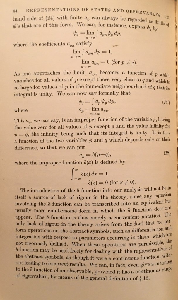
The δ function is thus merely a convenient notation … we perform operations on the abstract symbols, such as differentiation and integration …

PAM Dirac (1930)

The mathematics behind the “glitch” has a long history that began in the golden era of French analysis with the mathematicians Cauchy and Fourier, was employed by the electrical engineer Heaviside, and ultimately fell into the fertile hands of the quantum physicist, Paul Dirac, after whom it is named.

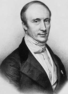
Augustin-Louis Cauchy (1815)

The French mathematician and physicist Augustin-Louis Cauchy (1789 – 1857) has lent his name to a wide array of theorems, proofs and laws that are still in use today. In mathematics, he was one of the first to establish “modern” functional analysis and especially complex analysis. In physics he established a rigorous foundation for elasticity theory (including the elastic properties of the so-called luminiferous ether).

Augustin-Louis Cauchy

In the early days of the 1800’s Cauchy was exploring how integrals could be used to define properties of functions.  In modern terminology we would say that he was defining kernel integrals, where a function is integrated over a kernel to yield some property of the function.

In 1815 Cauchy read before the Academy of Paris a paper with the long title “Theory of wave propagation on a surface of a fluid of indefinite weight”.  The paper was not published until more than ten years later in 1827 by which time it had expanded to 300 pages and contained numerous footnotes.  The thirteenth such footnote was titled “On definite integrals and the principal values of indefinite integrals” and it contained one of the first examples of what would later become known as a generalized distribution.  The integral is a function F(μ) integrated over a kernel

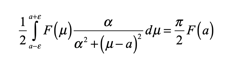
Cauchy lets the scale parameter α be “an infinitely small number”.  The kernel is thus essentially zero for any values of μ “not too close to α”.  Today, we would call the kernel given by

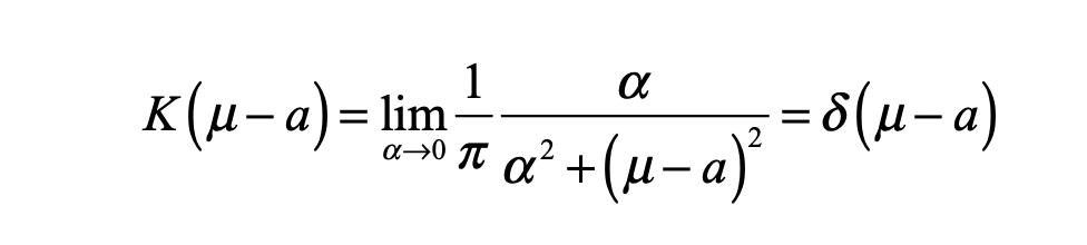
in the limit that α vanishes, “the delta function”.

Cauchy’s approach to the delta function is today one of the most commonly used descriptions of what a delta function is.  It is not enough to simply say that a delta function is an infinitely narrow, infinitely high function whose integral is equal to unity.  It helps to illustrate the behavior of the Cauchy function as α gets progressively smaller, as shown in Fig. 1. 

Fig. 1 Cauchy function for decreasing scale factor α approaches a delta function in the limit.

In the limit as α approaches zero, the function grows progressively higher and progressively narrower, but the integral over the function remains unity.

Joseph Fourier (1822)

The delayed publication of Cauchy’s memoire kept it out of common knowledge, so it can be excused if Joseph Fourier (1768 – 1830) may not have known of it by the time he published his monumental work on heat in 1822.  Perhaps this is why Fourier’s approach to the delta function was also different than Cauchy’s. 

Fourier noted that an integral over a sinusoidal function, as the argument of the sinusoidal function went to infinity, became independent of the limits of integration. He showed

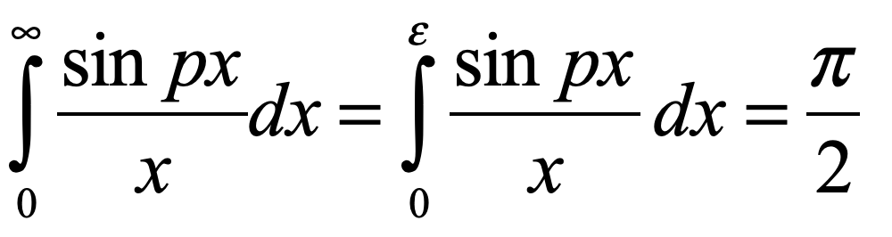
when ε << 1/p as p went to infinity. In modern notation, this would be the delta function defined through the “sinc” function

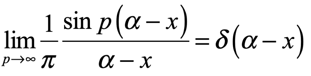
and Fourier noted that integrating this form over another function f(x) yielded the value of the function f(α) evaluated at α, rediscovering the results of Cauchy, but using a sinc(x) function in Fig. 2 instead of the Cauchy function of Fig. 1.

Fig. 2 Sinc function for increasing scale factor p approaches a delta function in the limit.

George Green’s Function (1829)

A history of the delta function cannot be complete without mention of George Green, one of the most remarkable British mathematicians of the 1800’s.  He was a miller’s son who had only one year of education and spent most of his early life tending to his father’s mill.  In his spare time, and to cut the tedium of his work, he read the most up-to-date work of the French mathematicians, reading the papers of Cauchy and Poisson and Fourier, whose work far surpassed the British work at that time.  Unbelievably, he mastered the material and developed new material of his own, that he eventually self published.  This is the mathematical work that introduced the potential function and introduced fundamental solutions to unit sources—what today would be called point charges or delta functions.  These fundamental solutions are equivalent to the modern Green’s function, although they were developed rigorously much later by Courant and Hilbert and by Kirchhoff.

George Green’s flour mill in Sneinton, England.

The modern idea of a Green’s function is simply the system response to a unit impulse—like throwing a pebble into a pond to launch expanding ripples or striking a bell.  To obtain the solutions for a general impulse, one integrates over the fundamental solutions weighted by the strength of the impulse.  If the system response to a delta function impulse at x = a, that is, a delta function δ(x-a), is G(x-a), then the response of the system to a distributed force f(x) is given by

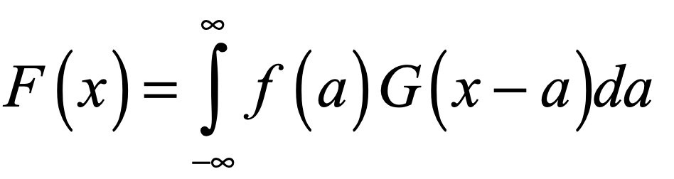
where G(x-a) is called the Green’s function.

Fig. Principle of Green’s function. The Green’s function is the system response to a delta-function impulse. The net system response is the integral over all the individual system responses summed over each of the impulses.

Oliver Heaviside (1893)

Oliver Heaviside (1850 – 1925) tended to follow his own path, independently of whatever the mathematicians were doing.  Heaviside took particularly pragmatic approaches based on physical phenomena and how they might behave in an experiment.  This is the context in which he introduced once again the delta function, unaware of the work of Cauchy or Fourier.

Oliver Heaviside

Heaviside was an engineer at heart who practiced his art by doing. He was not concerned with rigor, only with what works. This part of his personality may have been forged by his apprenticeship in telegraph technology helped by his uncle Charles Wheatstone (of the Wheatstone bridge). While still a young man, Heaviside tried to tackle Maxwell on his new treatise on electricity and magnetism, but he realized his mathematics were lacking, so he began a project of self education that took several years. The product of those years was his development of an idiosyncratic approach to electronics that may be best described as operator algebra. His algebra contained mis-behaved functions, such as the step function that was later named after him. It could also handle the derivative of the step function, which is yet another way of defining the delta function, though certainly not to the satisfaction of any rigorous mathematician—but it worked. The operator theory could even handle the derivative of the delta function.

The Heaviside function (step function) and its derivative the delta function.

Perhaps the most important influence by Heaviside was his connection of the delta function to Fourier integrals. He was one of the first to show that

which states that the Fourier transform of a delta function is a complex sinusoid, and the Fourier transform of a sinusoid is a delta function. Heaviside wrote several influential textbooks on his methods, and by the 1920’s these methods, including the Heaviside function and its derivative, had become standard parts of the engineer’s mathematical toolbox.

Given the work by Cauchy, Fourier, Green and Heaviside, what was left for Paul Dirac to do?
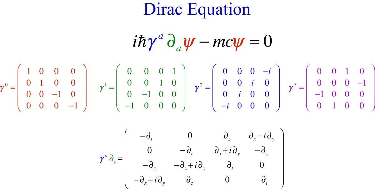
Paul Dirac (1930)

Paul Dirac (1902 – 1984) was given the moniker “The Strangest Man” by Niels Bohr during his visit to Copenhagen shortly after he had received his PhD.  In part, this was because of Dirac’s internal intensity that could make him seem disconnected from those around him. When he was working on a problem in his head, it was not unusual for him to start walking, and by the time he he became aware of his surroundings again, he would have walked the length of the city of Copenhagen. And his solutions to problems were ingenious, breaking bold new ground where others, some of whom were geniuses themselves, were fumbling in the dark.

P. A. M. Dirac

Among his many influential works—works that changed how physicists thought of and wrote about quantum systems—was his 1930 textbook on quantum mechanics. This was more than just a textbook, because it invented new methods by unifying the wave mechanics of Schrödinger with the matrix mechanics of Born and Heisenberg.

In particular, there had been a disconnect between bound electron states in a potential and free electron states scattering off of the potential. In the one case the states have a discrete spectrum, i.e. quantized, while in the other case the states have a continuous spectrum. There were standard quantum tools for decomposing discrete states by a projection onto eigenstates in Hilbert space, but an entirely different set of tools for handling the scattering states.

Yet Dirac saw a commonality between the two approaches. Specifically, eigenstate decomposition on the one hand used discrete sums of states, while scattering solutions on the other hand used integration over a continuum of states. In the first format, orthogonality was denoted by a Kronecker delta notation, but there was no equivalent in the continuum case—until Dirac introduced the delta function as a kernel in the integrand. In this way, the form of the equations with sums over states multiplied by Kronecker deltas took on the same form as integrals over states multiplied by the delta function.

Page 64 of Dirac’s 1930 edition of Quantum Mechanics.

In addition to introducing the delta function into the quantum formulas, Dirac also explored many of the properties and rules of the delta function. He was aware that the delta function was not a “proper” function, but by beginning with a simple integral property as a starting axiom, he could derive virtually all of the extended properties of the delta function, including properties of its derivatives.

Mathematicians, of course, were appalled and were quick to point out the insufficiency of the mathematical foundation for Dirac’s delta function, until the French mathematician Laurent Schwartz (1915 – 2002) developed the general theory of distributions in the 1940’s, which finally put the delta function in good standing.

Dirac’s introduction, development and use of the delta function was the first systematic definition of its properties. The earlier work by Cauchy, Fourier, Green and Heaviside had all touched upon the behavior of such “spiked” functions, but they had used it in passing. After Dirac, physicists embraced it as a powerful new tool in their toolbox, despite the lag in its formal acceptance by mathematicians, until the work of Schwartz redeemed it.

By David D. Nolte Feb. 17, 2022


Bibliography

V. Balakrishnan, “All about the Dirac Delta function(?)”, Resonance, Aug., pg. 48 (2003)

M. G. Katz. “Who Invented Dirac’s Delta Function?”, Semantic Scholar (2010).

J. Lützen, The prehistory of the theory of distributions. Studies in the history of mathematics and physical sciences ; 7 (Springer-Verlag, New York, 1982).

Dirac: From Quantum Field Theory to Antimatter

Paul Adrian Maurice Dirac (1902 – 1984) was given the moniker of “the strangest man” by Niels Bohr while he was reminiscing about the many great scientists with whom he had worked over the years [1].  It is a moniker that resonates with the innumerable “Dirac stories” that abound in the mythology of the hallways of physics departments around the world.  Dirac was awkward, shy, a loner, rarely said anything, was completely literal, had not the slightest comprehension of art or poetry, nor any clear understanding of human interpersonal interaction.  Dirac was also brilliant, providing the theoretical foundation for the central paradigm of modern physics—quantum field theory.  The discovery of the Higgs boson in 2012, a human achievement that capped nearly a century of scientific endeavor, rests solidly on the theory of quantum fields that permeate space.  The Higgs particle, when it pops into existence at the Large Hadron Collider in Geneva, is a singular quantum excitation of the Higgs field, a field that usually resides in a vacuum state, frothing with quantum fluctuations that imbue all particles—and you and me—with mass.  The Higgs field is Dirac’s legacy.

… all of a sudden he had a new equation with four-dimensional space-time symmetry.

Copenhagen and Bohr

Although Dirac as a young scientist was initially enthralled with relativity theory, he was working under Ralph Fowler (1889 – 1944) in the physics department at Cambridge in 1923 when he had the chance to read advanced proofs of Heisenberg’s matrix mechanics paper.  This chance event launched him on his own trajectory in quantum theory.  After Dirac was awarded his doctorate from Cambridge in 1926, he received a stipend that sent him to work with Niels Bohr (1885 – 1962) in Copenhagen—ground zero of the new physics. During his time there, Dirac became famous for taking long walks across Copenhagen as he played about with things in his mind, performing mental juggling of abstract symbols, envisioning how they would permute and act.  His attention was focused on the electromagnetic field and how it interacted with the quantized states of atoms.  Although the electromagnetic field was the classical field of light, it was also the quantum field of Einstein’s photon, and he wondered how the quantized harmonic oscillators of the electromagnetic field could be generated by quantum wavefunctions acting as operators.  But acting on what?  He decided that, to generate a photon, the wavefunction must operate on a state that had no photons—the ground state of the electromagnetic field known as the vacuum state.

            In late 1926, nearing the end of his stay in Copenhagen with Bohr, Dirac put these thoughts into their appropriate mathematical form and began work on two successive manuscripts.  The first manuscript contained the theoretical details of the non-commuting electromagnetic field operators.  He called the process of generating photons out of the vacuum “second quantization”.  This phrase is a bit of a misnomer, because there is no specific “first quantization” per se, although he was probably thinking of the quantized energy levels of Schrödinger and Heisenberg.  In second quantization, the classical field of electromagnetism is converted to an operator that generates quanta of the associated quantum field out of the vacuum (and also annihilates photons back into the vacuum).  The creation operators can be applied again and again to build up an N-photon state containing N photons that obey Bose-Einstein statistics, as they must, as required by their integer spin, agreeing with Planck’s blackbody radiation. 

            Dirac then went further to show how an interaction of the quantized electromagnetic field with quantized energy levels involved the annihilation and creation of photons as they promoted electrons to higher atomic energy levels, or demoted them through stimulated emission.  Very significantly, Dirac’s new theory explained the spontaneous emission of light from an excited electron level as a direct physical process that creates a photon carrying away the energy as the electron falls to a lower energy level.  Spontaneous emission had been explained first by Einstein more than ten years earlier when he derived the famous A and B coefficients, but Einstein’s arguments were based on the principle of detailed balance, which is a thermodynamic argument.  It is impressive that Einstein’s deep understanding of thermodynamics and statistical mechanics could allow him to derive the necessity of both spontaneous and stimulated emission, but the physical mechanism for these processes was inferred rather than derived. Dirac, in late 1926, had produced the first direct theory of photon exchange with matter.  This was the birth of quantum electrodynamics, known as QED, and the birth of quantum field theory [2].

Fig. 1 Paul Dirac in his early days.

Göttingen and Born

            Dirac’s next stop on his postodctoral fellowship was in Göttingen to work with Max Born (1882 – 1970) and the large group of theoreticians and mathematicians who were like electrons in a cloud orbiting around the nucleus represented by the new quantum theory.  Göttingen was second only to Copenhagen as the Mecca for quantum theorists.  Hilbert was there and von Neumann too, as well as the brash American J. Robert Oppenheimer (1904 – 1967) who was finishing his PhD with Born.  Dirac and Oppenheimer struck up an awkward friendship.  Oppenheimer was considered arrogant by many others in the group, but he was in awe of Dirac who arrived with his manuscript on quantum electrodynamics ready for submission.  Oppenheimer struggled at first to understand Dirac’s new approach to quantizing fields, but he quickly grasped the importance, as did Pascual Jordan (1902 – 1980), who was also in Göttingen.

            Jordan had already worked on ideas very close to Dirac’s on the quantization of fields.  He and Dirac seemed to be going down the same path, independently arriving at very similar conclusions around the same time.  In fact, Jordan was often a step ahead of Dirac, tending to publish just before Dirac, as with non-commuting matrices, transformation theory and the relationship of canonical transformations to second quantization.  However, Dirac’s paper on quantum electrodynamics was a masterpiece in clarity and comprehensiveness, launching a new field in a way that Jordan had not yet achieved with his own work.  But because of the closeness of Jordan’s thinking to Dirac’s, he was able to see immediately how to extend Dirac’s approach.  Within the year, he published a series of papers that established the formalism of quantum electrodynamics as well as quantum field theory.  With Pauli, he systematized the operators for creation and annihilation of photons [3].  With Wigner, he developed second quantization for de Broglie matter waves, defining creation and annihilation operators that obeyed the Pauli exclusion principle of electrons[4].  Jordan was on a roll, forging ahead of Dirac on extensions of quantum electrodynamics and field theory, but Dirac was about to eclipse Jordan once and for all.

St. John’s at Cambridge

            At the end of the Spring semester in 1927, Dirac was offered a position as a fellow of St. John’s College at Cambridge, which he accepted, returning to England to begin his life as a college professor.  During the summer and into the Fall, Dirac returned to his first passion in physics, relativity, which had yet to be successfully incorporated into quantum physics.  Oskar Klein and Walter Gordon had made initial attempts at formulating relativistic quantum theory, but they could not correctly incorporate the spin properties of the electron, and their wave equation had the bad habit of producing negative probabilities.  Probabilities went negative because the Klein-Gordon equation had two time derivatives instead of one.  The reason it had two (while the non-relativistic Schrödinger equation has only one) is because space-time symmetry required the double space derivative of the Schrödinger equation to be paired with a double time derivative.  Dirac, with creative insight, realized that the problem could be flipped by requiring the single time derivative to be paired with a single space derivative.  The problem was that a single space derivative did not seem to make any sense [5].

St. John’s College at Cambridge

            As Dirac puzzled how to get an equation with only single derivatives, he was playing around with Pauli spin matrices and hit on a simple identity that related the spin matrices to the electron momentum.  At first he could not get the identity to apply to four-dimensional relativistic momenta using the usual 2×2 spin matrices.  Then he realized that four-dimensional space-time could be captured if he expanded Pauli’s 2×2 spin matrices to 4×4 spin matrices, and all of a sudden he had a new equation with four-dimensional space-time symmetry with single derivatives on space and time.  As a test of his new equation, he calculated fine details of the experimentally-measured hydrogen spectrum, known as the fine structure, which had resisted theoretical explanation, and he derived answers in close agreement with experiment.  He also showed that the electron had spin-1/2, and he calculated its magnetic moment.  He finished his manuscript at the end of the Fall semester in 1927, and the paper was published in early 1928[6].  His relativistic quantum wave equation was an instant sensation, becoming known for all time as “the Dirac Equation”.  He had succeeded at finding a correct and long-sought relativistic quantum theory where many others had failed, such as Oskar Klein and Paul Gordon.  It was a crowning achievement, placing Dirac firmly in the firmament of the quantum theorists.

Fig. 1 The relativistic Dirac equation. The wavefunction is a four-component spinor. The gamma-del product is a 4×4 matrix operator. The time and space derivatives are both first-order operators.

Antimatter

            In the process of ridding the Klein-Gordon equation of negative probability, which Dirac found abhorent, his new equation created an infinite number of negative energy states, which he did not find abhorent.  It is perhaps a matter of taste what one theoriest is willing to accept over another, and for Dirac, negative energies were better than negative probabilities.  Even so, one needed to deal with an infinite number of negative energy states in quantum theory, because they are available to quantum transitions.  In 1929 and 1930, as Dirac was writing his famous textbook on quantum theory, he became intrigued by the similarity between the positive and negative electron states of the vacuum and the energy levels of valence electrons on atoms.  An electron in a state outside a filled electron shell behaves very much like a single-electron atom, like sodium and lithium with their single valence electrons.  Conversely, an atomic shell that has one electron less than a full complement can be described as having a “hole” that behaves “as if” it were a positive particle.  It is like a bubble in water.  As water sinks, the bubble rises to the top of the water level.  For electrons, if all the electrons go one way in an electric field, then the hole goes the opposite direction, like a positive charge. 

            Dirac took this analogy of nearly-filled atomic shells and applied it to the vacuum states of the electron, viewing the filled negative energy states like the filled electron shells of atoms.  If there is a missing electron, a hole in this infinite sea, then it would behave as if it had positive charge.  Initially, Dirac speculated that the “hole” was the proton, and he even wrote a paper on that possibility.  But Oppenheimer pointed out that the idea was inconsistent with observations, especially the inability of the electron and proton to annihilate, and that the ground state of the infinite electron sea must be completely filled. Hermann Weyl further pointed out that the electron-proton theory did not have the correct symmetry, and Dirac had to rethink.  In early 1931 he hit on an audacious solution to the puzzle.  What if the hole in the infinite negative energy sea did not just behave like a positive particle, but actually was a positive particle, a new particle that Dirac dubbed the “anti-electron”?  The anti-electron would have the same mass as the electron, but would have positive charge. He suggested that such particles might be generated in high-energy collisions in vacuum, and he finished his paper with the suggestion that there also could be an anti-proton with the mass of the proton but with negative charge.  In this singular paper, titled “Quantized Singularities of the Electromagnetic Field” published in 1931, Dirac predicted the existence of antimatter.  A year later the positron was discovered by Carl David Anderson at Cal Tech.  Anderson had originally called the particle the positive electron, but a journal editor of the Physical Review changed it to positron, and the new name stuck.

Fig. 3 An electron-positron pair is created by the absorption of a photon (gamma ray). Positrons have negative energy and can be viewed as a hole in a sea of filled electron states. (Momentum conservation is satisfied if a near-by heavy particle takes up the recoil momentum.)

            The prediction and subsequent experimental validation of antmatter stands out in the history of physics in the 20th Century.  In previous centuries, theory was performed mainly in the service of experiment, explaining interesting new observed phenomena either as consequences of known physics, or creating new physics to explain the observations.  Quantum theory, revolutionary as a way of understanding nature, was developed to explain spectroscopic observations of atoms and molecules and gases.  Similarly, the precession of the perihelion of Mercury was a well-known phenomenon when Einstein used his newly developed general relativity to explain it.  As a counter example, Einstein’s prediction of the deflection of light by the Sun was something new that emerged from theory.  This is one reason why Einstein became so famous after Eddington’s expedition to observe the deflection of apparent star locations during the total eclipse.  Einstein had predicted something that had never been seen before.  Dirac’s prediction of the existence of antimatter similarly is a triumph of rational thought, following the mathematical representation of reality to an inevitable conclusion that cannot be ignored, no matter how wild and initially unimaginable it is.  Dirac went on to receive the Nobel prize in Physics in 1933, sharing the prize that year with Schrödinger (Heisenberg won it the previous year in 1932).


Read all the stories behind the history of quantum field theory, in Galileo Unbound from Oxford Press:


References

[1] Framelo, “The Strangest Man: The Hidden Life of Paul Dirac” (Basic Books, 2011)

[2] Dirac, P. A. M. (1927). “The quantum theory of the emission and absorption of radiation.” Proceedings of the Royal Society of London Series A114(767): 243-265.;  Dirac, P. A. M. (1927). “The quantum theory of dispersion.” Proceedings of the Royal Society of London Series A114(769): 710-728.

[3] Jordan, P. and W. Pauli, Jr. (1928). “To quantum electrodynamics of free charge fields.” Zeitschrift Fur Physik 47(3-4): 151-173.

[4] Jordan, P. and E. Wigner (1928). “About the Pauli’s equivalence prohibited.” Zeitschrift Fur Physik 47(9-10): 631-651.

[5] This is because two space derivatives measure the curvative of the wavefunction which is related to the kinetic energy of the electron.

[6] Dirac, P. A. M. (1928). “The quantum theory of the electron.” Proceedings of the Royal Society of London Series A 117(778): 610-624.;  Dirac, P. A. M. (1928). “The quantum theory of the electron – Part II.” Proceedings of the Royal Society of London Series A118(779): 351-361.