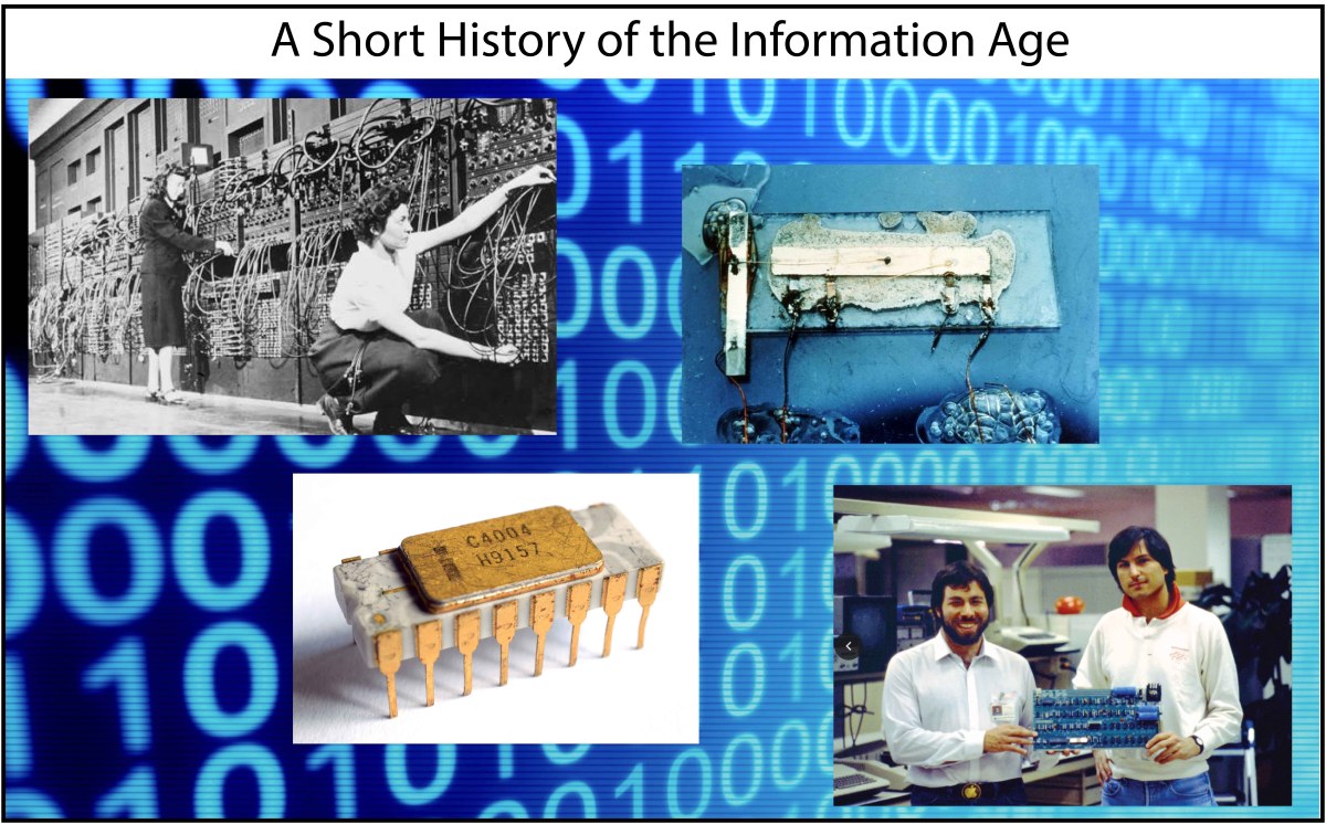
A Short History of the Information Age

A Short History of the Information Age

We are immersed in information, bathed in bits. 

Information surrounds us, informs us, guides us, protects us.  Without it, life could not exist.  Without it, the universe could not exist—because the universe might very well be information

Despite the ubiquity of information, the Information Age, as we call it, is quite young, only about 80 years old.  Everyone alive today has spent most, or all, of their lives watching it unfold.  Only octogenarians or older have any hope of remembering what life was like before the revolution.

The Information Age is defined by the dominance of digital information across society, economics and culture.  Information in a more raw form has been guiding human society ever since the invention of language about 500,000 years ago.  The invention of writing gave it a material boost 5000 years ago, and Gutenberg accelerated the process 500 years ago. But the threshold to the Information Age was crossed in 1945 with the invention of the ENIAC, the first digital computer.  From that moment, the analog world began to slip away, replaced by bits. The global amount of stored digital information surpassed analog storage (books, phonographs, photographs, audio tapes) in 2002. 

It may be too early today to gain the distance needed for a frank assessment, but the first 40 years were the real go-go years, when most of the underlying technology was invented.  Here is a short history of those first forty years of the Information Age, beginning with ENIAC in 1945 through the invention of the World Wide Web in 1989.

The ENIAC, University of Pennsylvania (1945)

The Information Age and the Computer Age are nearly synonymous.  The chief function of information is control, and the chief mechanism by which one stream of information controls another is in a computer. 
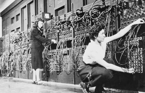
Marlyn Wescoff (left) and Ruth Lichterman programming the ENIAC computer
Marlyn Wescoff (left) and Ruth Lichterman programming the ENIAC.

The first fully functional electronic computer was the ENIAC built at the University of Pennsylvania in 1945 by physicist John Mauchly and engineer J. Eckert in collaboration with John von Neumann.  The three invented the stored-program architecture that consisted of a central processing unit (CPU), a memory and input/output ports.  It weighed 27 tons and consumed 150 kWatts of electricity, but it was 10 times faster than mechanical calculators.

The Transistor, Bell Labs (1947)

In the years from WWII to the notorious breakup of AT&T by federal district court judge Harold Green in 1984, Bell Labs was the apex R&D lab in the world.  Even in 1988, when I arrived at Holmdel, NJ, to begin my post-doc position with Alastair Glass in the Optical Materials Department, it still retained the glow of its halcyon days.  Nothing was impossible, and research ran at a furious pace.
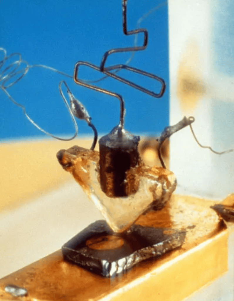
An image of the first transistor made from a Germanium semiconductor.
The first transistor.

The accelerating use of electronics during WWII had led to an intense research program to replace large, expensive, over-heating vacuum tubes with a compact solid-state device.  At Bell Labs, John Bardeen, Walter Brattain and William Shockley succeeded in controlling a current with a voltage in a transistor constructed of germanium in 1947.  The germanium was soon replaced by silicon that had superior properties, especially its oxide properties that enabled the operation of field effect transistors (FETs). 
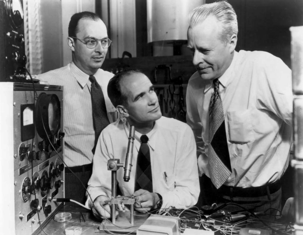
Photo of Bardeen, Shockley and Brattain with the first transistor.
Bardeen, Schockley and Brattain with the first transistor.

Information Theory, Bell Labs (1948)

The Information Age would not be a recognized technological age of modern society without a theory to go with it.  This was provided by Claude Shannon of Bell Labs in 1948, who recognized that information was related to a concept that Ludwig Boltzmann had derived 70 years earlier—Entropy.  The equation chiseled into stone on Boltzmann’s memorial in Vienna, Austria, states simply that entropy is proportional to the logarithm of the probability of states.
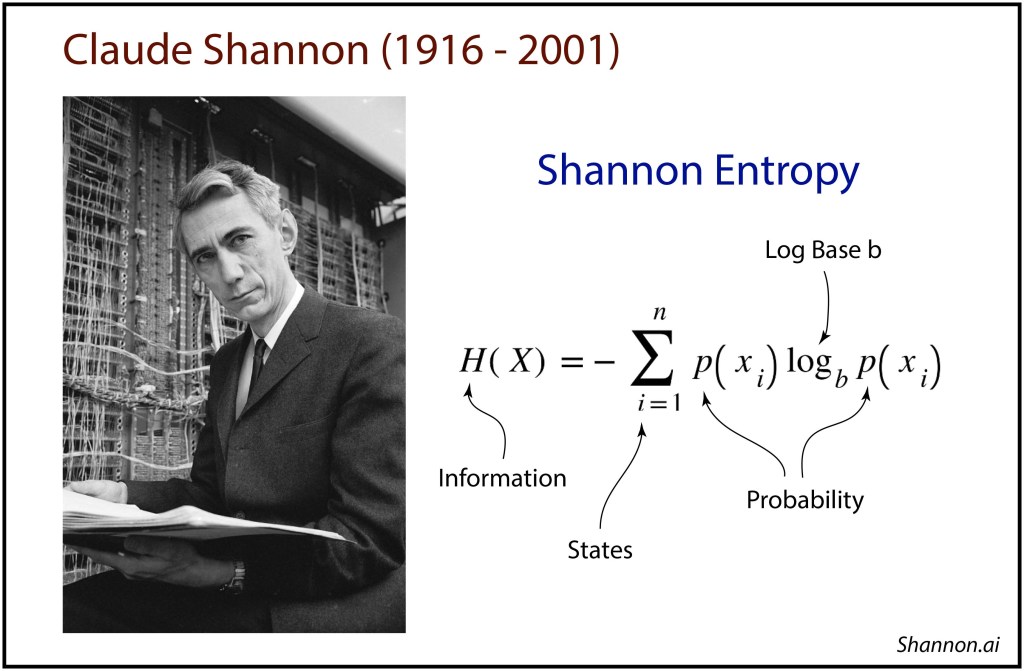
Claude Shannon and the mathematical formula for information based on entropy

Shannon showed that information is a measure of “surprise”, meaning that is it the likelihood of observing something unexpected.  If there is no surprise in a message, like a string of ones “1111111 ..”, then the message carries no information.  It is only when the message is structured “1011000110010101” that it carries information to distinguish one bit from the next.  Information is greatest when the surprise is greatest, which is also the highest entropy.

This concept of information is un-intuitive, but it ends up explaining almost every aspect of the flow of information through any dynamical or complex system.  Physicists like John Wheeler of Princeton and Seth Lloyd of MIT went so far as to claim that the physics of reality is in reality the physics of information.

Magnetic Hard Disk Drive, IBM (1953)

When I first learned to run computer programs on a mainframe computer at Cornell University in 1978, the first step in the process was converting my computer code into punched IBM cards that were fed into a mechanical reader.  Even then, it was a hold-over from a by-gone age when all computer memory was mechanical, either in the form of punched cards or magnetic tape.
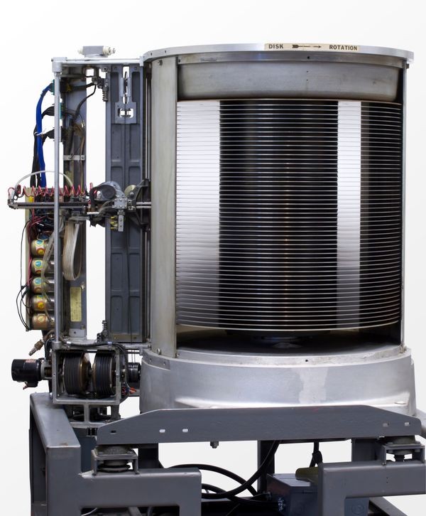
Photo of the first IBM hard drive system
The RAMAC 350 by IBM.

That all changed with the IBM 350 Disk Storage Unit that used spinning magnetic disks and a read head that floated on a cushion of air just a few mils above the disk surface.  This was the first commercial hard drive, invented at the IBM San Jose research facility in 1953 by Reynold Johnson, a former high-school teacher who had a knack for invention.  The key feature of the hard drive was its ability to provide random-access to stored information.  The unit was bigger than a refrigerator and weighed a ton while only having a storage capacity of 5 MB.  But the tech has scaled well, and today 8 TB hard drives the size of a pocket book are commonplace.

Integrated Circuit, Texas Instruments (1958)

The invention of the integrated circuit was a pivotal moment that launched electronic miniaturization, ushering in increasingly complex function into increasingly smaller packages.  The miniaturization trend has been going strong for 60 years and continues today.
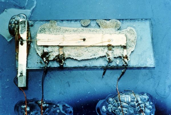
Photo of Jack Kilby's first integrated circuit.
First integrated circuit by Jack Kilby of Texas Instruments.

The integrated circuit solved the problem of spaghetti wiring needed to wire transistors together with capacitors and resistors on circuit boards.  By integrating the construction of wires, transistors, capacitors and resistors onto a semiconductor chip, all the mess is removed and each of the elements can be reduced in size.

The integrated circuit was invented by Jack Kilby of Texas Instruments.  Shortly after joining the company, he was stranded while others were away on vacation (he had not accrued any vacation time yet), so he thought of the idea of integrating the different circuit elements onto a single chip.  He built the first demo out of a chip of germanium

The Laser, Hughes Research Lab (1960)

Ted Maiman, the inventor of the laser, was a wanderer.  When given the opportunity to work with a Nobel prize winner at Stanford, he instead used his life savings to take a trip around the world.  Settling back into research life after his trip, he got a job at Hughes Research Lab, the research arm of the Hughes Corporation founded by the eccentric Howard Hughes. 
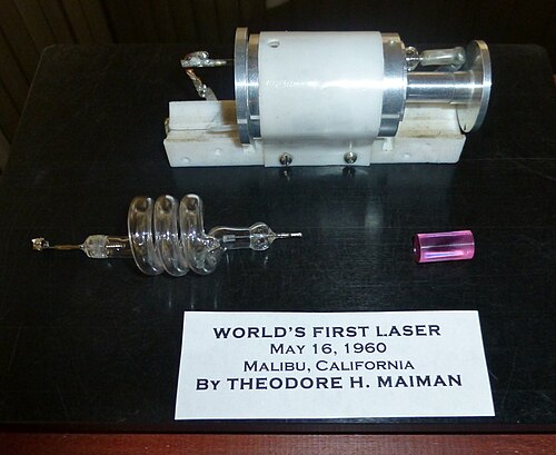
His first job at the lab was to improve on the ruby maser (micro-wave amplification by stimulated emission) but he wandered off track and began pursuing light emission—the so-called optical maser.  The common wisdom was that ruby would not lase, and Ali Javan at Bell Labs was close to completing the first HeNe laser.  Yet Maiman tried anyway by wrapping an intense flash tube around a rod of ruby with polished mirror faces.  On May16, 1960, he and his technician, Irnee D’Haenens, slowly increased the voltage to the flash tube until the room suddenly glowed red when the rod emitted red laser radiation.  D’Haenens was color blind and could not normally see red, but the laser light was so bright that even the few red receptors in his eyes picked up the light.  He saw the color red for the first time in his life! (Read more about the discovery of the laser in Chapter 8 of Interference (Oxford University Press (2023)).

T-Carrier, Bell Labs (1962)

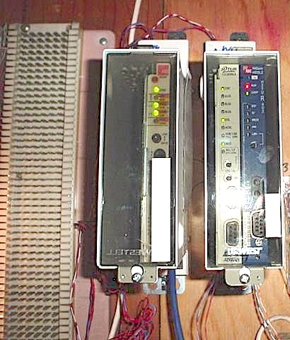
Information does little good if it cannot be transmitted from place to place.  In 1962, engineers at Bell Labs introduced the T-carrier, a method to transmit digital information over simple twisted-pair copper wires.  The master stroke of this invention is that it took the standard wire that was designed for a single analog phone conversation and sent 24 simultaneous conversations in digital form down the same wire.  By the early 1960’s the US had nearly 400 million miles of twisted pair laid down that would have cost a fortune to replace, but the Bell engineers “repurposed” it, extending the capacity by multiplexing, eventually pushing the multiplex level up to 96 simultaneous conversations.  One of the engineers responsible for this technological advance was John Mayo, who became the seventh president of Bell Labs in 1991.
Moore’s Law, Fairchild Semiconductor (1965)

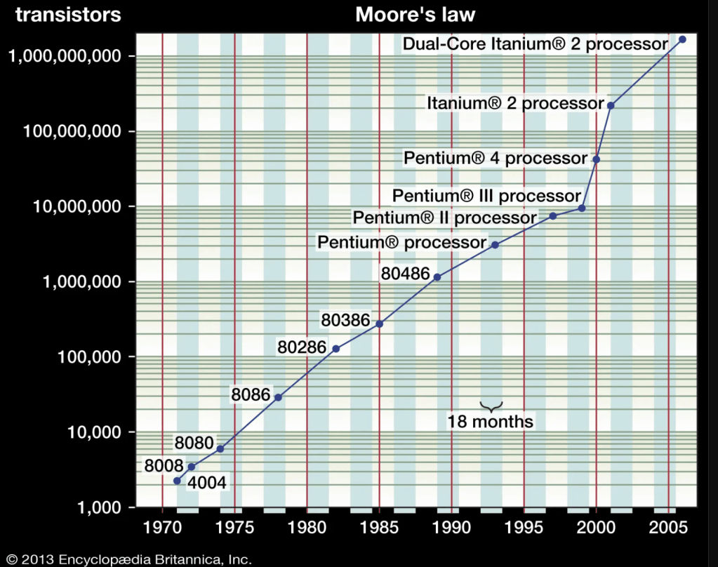
In 1965 Gordon Moore, the director of research at Fairchild Semiconductor in San Jose, California, was asked to contribute a short opinion piece to a special issue of an electronics magazine.  In the article he noted that the complexity of integrated silicon circuits was doubling about every year, and he projected that the trend would continue for the next ten years.  He revisited his prediction in 1975, noting that the trend would likely continue until 1980, after which it would adjust to a doubling every two years into the foreseeable future.  His prediction was essentially correct, and “Moore’s Law” has been on track for over half a century.  Numerous other technologies are now following their own form of Moore’s Law.
Fiber Optics, Standard Communications Laboratory, UK (1966)

In the early days of fiber optic research, shortly after 1960, scientists could not send light a hundred meters without losing nearly all of the intensity. The first breakthrough came in 1966 with the suggestion by Charles Kao, working a the Standard Communications Laboratory in England that a light-guiding core of high-density glass could be surrounded with an outer cladding of lower density glass. The lower-density cladding still allowed total internal reflection, while shielding the guided light from the rough surface of the fiber. This clad fiber solved one of the impediments to getting light to travel long distances, but there was still the problem of absorption by impurities in glass.
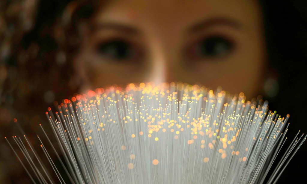
The second breakthrough came in 1970 when researchers at Corning Glass showed that, by using a special fabrication technique called chemical vapor deposition (CVD), the fibers could be made so pure that the absorption was minimized. They showed that light intensity in the fiber would drop only 99 percent over one kilometer. Though this sounds like a big drop in intensity, it was a critical threshold toward which everyone had been working. With this degree of transparency, a fiber system could have a repeater (a photodetector that receives the signal, and a laser that relaunches it down the next segment of fiber) spaced as far as 1 – 2 km apart. This was a magic number because it was the same repeat distance that was being used by electronic transmission. If it was good enough for telephone wires, it should be good enough for fibers. (Read more about the discovery of fiber optics in Chapter 6 of Mind at Light Speed (Free Press (2001))

SRAM Memory, RCA Laboratories (1968)

Core computer memory prior to 1965 was based on small magnetic ferrite rings threaded by small wires.  The devices were large and slow (by modern standards) and maxed out at about 8 MB.  Static Random Access Memory (SRAM) circuits would eventually replace core memory, but they had a modest start.  CMOS technology was invented at Fairchild Semiconductor in 1965 and was rapidly developed into TTL circuits as well as static RAM, but the capacity was initially only 288 bits.  RCA Laboratories integrated the CMOS into circuits that provided a long runway for scaling.  Today SRAM chips easily hold 64 MB of information while SRAM in CPU cores reach several GB.

CCD, Bell Labs (1969)

Light is one of the most ubiquitous and most information-rich probes of the world around us.  Although light moves in three dimensions, a two-dimensional cross section of light paths captures the essential information content.  Therefore, cameras are the quintessential collectors of information carried by light, and digital cameras are the front end to any downstream image processing using computers and telecommunications.
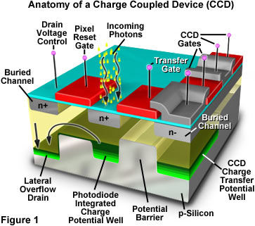
The charge-coupled device (CCD) was the breakthrough digital imaging technology of the Information Age, launching the revolution in commercial, industrial, scientific and personal imaging.  The CCD was invented at Bell Labs in 1969 by George Smith and Willard Boyle (who received the Nobel Prize in Physics for the invention in 2009) when they realized that MOS technology in silicon could transfer “buckets” (they called them “bubbles’) of electrons from one capacitor to an adjacent one on the chip, creating a “bucket brigade” of electrons along linear chains of capacitors.  The application of CCD technology specifically for imaging was demonstrate the next year in 1970.

Compact Disc, Pillips Corp. (1969)

The wavelength of light is about one micron (a millionth of a meter), so the storage of information on an optical disk has an ultra-high density of about 1 bit per square micron.  The first technology to try to access this data density was the compact disk of Klaas Compaan and later Kees Immink at Phillips Corporation.  CDs eventually reached a storage of 700 MB of data.  They were cheap to manufacture (pennies per disk) and easy to distribute (jewel cases) and replaced previous magnetic tape as the chief storage medium for music.  This was followed by DVDs with 5 GB for movies and later BluRay (shorter wavelength and multiple layers) in the early 2000’s with a storage of 25 GB of data.
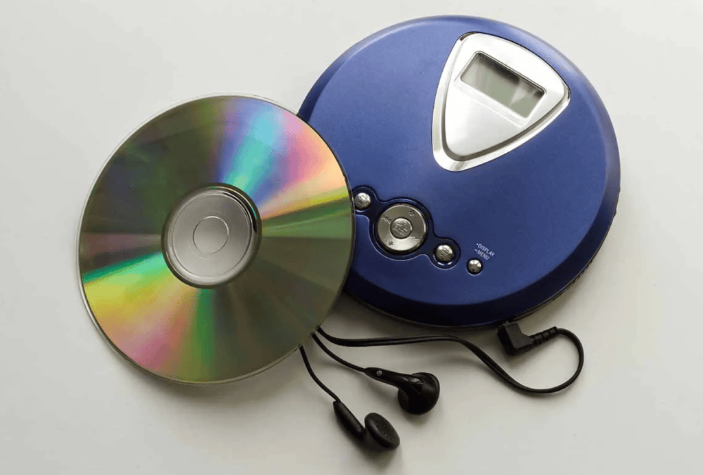
(As a personal aside, in the late 90’s, Marty Becker, a colleague of mine at Purdue, came into my office one day and asked my why CD’s reflected rainbow colors.  I didn’t know, but when I looked into it, I was amazed to find that the surface of a CD consisted of a billion little pits that each were a tiny optical interferometer.  (Optical interferometers are the most sensitive measurement system mankind has ever devised, capable of detecting the merger of two black holes from half a universe away.). This had been the brainchild of Klass Compaan and Piet Kramer of the Phillips Corporation in the Netherlands. 

About a year after I had talked with Marty, I was asked by Fred Regnier, another colleague at Purdue, how a physicist might measure thousands of different proteins to help the new field of proteomics.  I immediately thought of Compaan’s billion little interferometers and suggested that the little pits could be used like a billion little test tubes and use light to measure the protein reactions.  This was the origin of the BioCD, which went on to commercial success in the canine blood diagnostics market between 2010 and 2020.)

Intel 4004, Intel (1971)

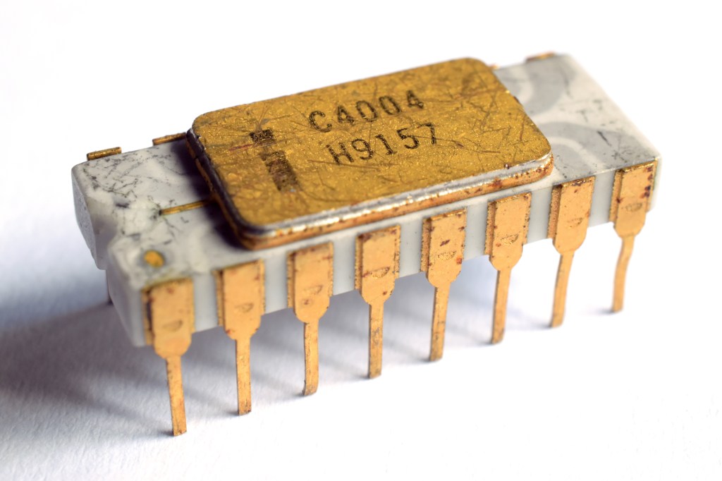
Transistors had already revolutionized circuit board electronics, but these were still bulky and expensive to fabricate.  A major technological breakthrough came with the integration of multiple transistors on a chip, and multiple chips in a package, creating significant computing power in the size of about 1 centimeter.  This was achieved by Intel with the release of the Intel 4004 microprocessor in 1971.  The fabrication was intrinsically scalable, putting successively more transistors onto chips, driving Moore’s Law for many decades.
Altair 8800, MITS (1975)

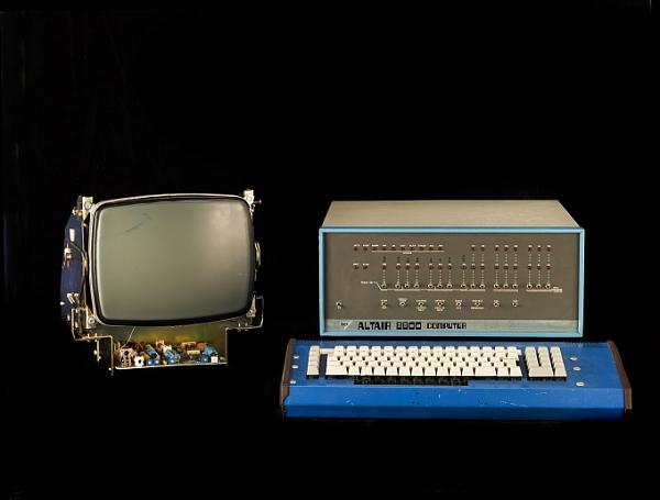
By combining microprocessor chips with memory and a user interface, the first personal computers came out as DIY electronics kits.  The first was the Altair 8800 released by MITS in 1975 as a hobbyist kit used for the first rudimentary computer games.
Apple II, Apple Corporation (1977)

Kits are fine for hobbyists, but personal computers could not penetrate mass markets until they became “appliances”.  This was achieved by Steve Wozniak and Steve Jobs at Apple in 1977 with the release of the Apple II that came with the VisiCalc program, the first spread-sheet application that saw widespread utility, known as a “killer app”.  The Commodore 64 microcomputer and the RadioShack TRS-80 were also early entries into the personal computer market.
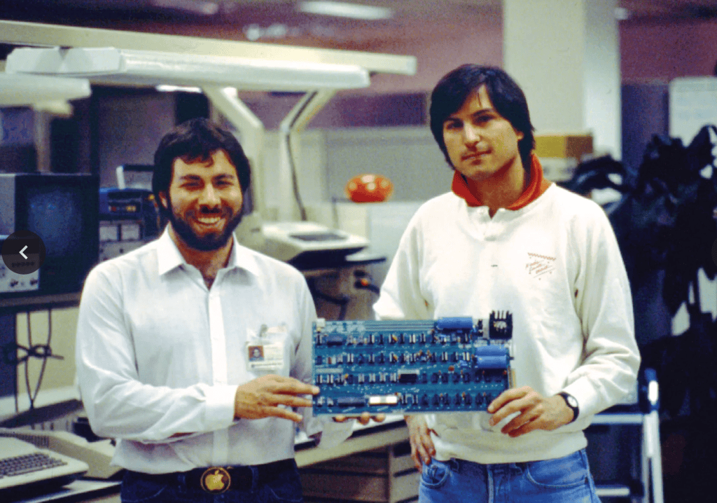
Steve Wozniak and Steve Jobs in 1976. Link.

Cell Phone, Motorola (1983)

The invention of the cell phone affected everyone by ushering in 24-7 with a vengeance. With the cell phone, no one is ever unavailable or out of touch or lost. It connected individuals into dense human networks.

The first cell phone call was made in 1973 by Martin Cooper of Motorola to his competitor at AT&T. It took another 10 years to settle all the regulatory issues and to build the first cell network before the Motorola DynaTAC 8000X was released to the public in 1983 operating on an AT&T network.
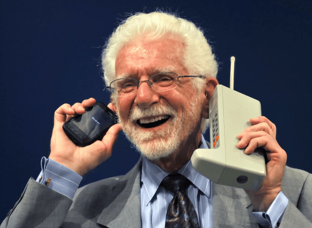
Photon of Martin Cooper holding the DynaTac 8000X along with a modern cell phone.
Martin Cooper holding the DynaTac 8000X along with a modern cell phone.

Handwriting Recognition, Bell Labs (1988)

When I joined Bell Labs in 1988, new employees were treated to a grand introduction to Bell Labs research by the president Arno Penzius, who had won the Nobel Prize in physics in 1978 for discovering the microwave background of the Big Bang.  We also were given tours of select labs where significant advances were being made.  One lab I visited was the handwriting recognition lab at Holmdel, NJ, where Yann LeCun was revolutionizing the recognition of handwritten numbers.
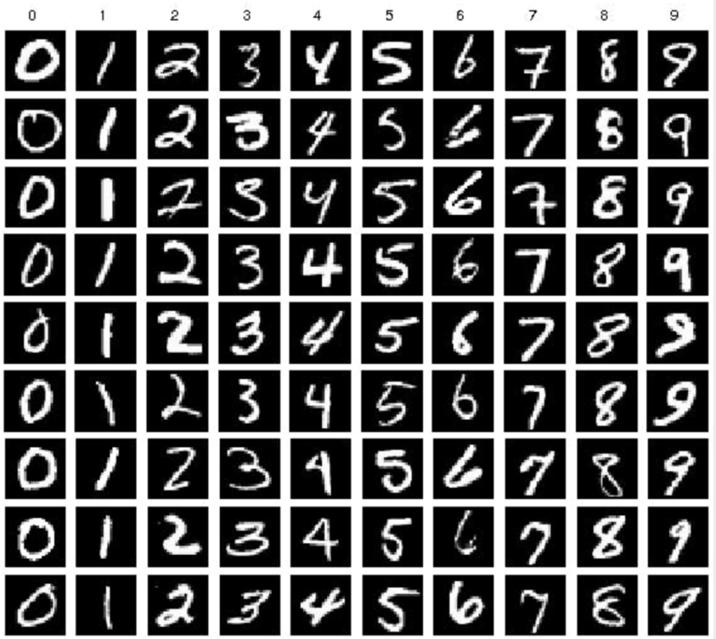
The MNIST data set
MNIST Number Set.

LeCun had joined Bell Labs the same year I did, coming from a post-doc with Geoff Hinton at Toronto where he had studied neural networks.  At Bell Labs, LeCun developed the convolutional neural network (CNN) to replace the fully connected layers of neurons that had routinely been used in previous networks.  The CNN, by using expanding fields of attention, required far fewer neural weights to train.  That year, the Bell Labs team tried out the new neural network architecture on scans of thousands of handwritten numbers provided by the US Postal Service from their facility in Buffalo, NY.  LeCun went on to become one of the leading figures in the AI revolution.

World Wide Web (1989)

The World Wide Web was invented by English computer scientist Tim Berners-Lee in March 1989 while working at CERN (the European Organization for Nuclear Research). Five years later, in a faculty meeting in the Physics Department at Purdue University, I was introduced to this new thing called the “World Wide Web” by an Physics IT staff. They told us we would need to learn how to use it because it would change how we did our jobs. None of us believed him—but teaching at the university today is almost unrecognizable to what it was in the early 90’s. And the same with daily life. The WWW changed everything from how we shop to how we read to how we communicate. It is the information conduit of the Information Age.
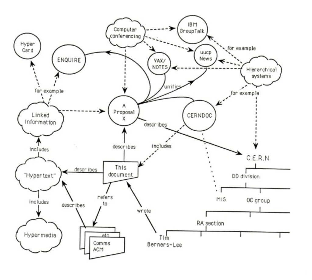
The first diagram of the internet by Berners'Lee
Berners-Lee’s diagram in his 1989 proposal for the web. Link.

Epilog

The Information Age proper began 80 years ago (although information has been with us since the start of the universe in the Big Bang). This short history has covered the first 40 years, so only about half of the period. Since 1989, the inventions of the first 40 years have matured and evolved, but are still mostly recognizable. Cell phones are still cell phones, just smaller and smarter. The internet now consumes our attention, but it uses the same hypertext technology as the first network at CERN.

But one thing has evolved that is about to remake human society—AI. It likely will change life in such radical ways that it will mark a discontinuity in human history. Born of the Information Age, AI may close that door and usher in a new Cognitive Age. How humans will participate in the new Age is an open question.

A short history of hyperspace

A Short History of Multiple Dimensions

Hyperspace by any other name would sound as sweet, conjuring to the mind’s eye images of hypercubes and tesseracts, manifolds and wormholes, Klein bottles and Calabi Yau quintics.  Forget the dimension of time—that may be the most mysterious of all—but consider the extra spatial dimensions that challenge the mind and open the door to dreams of going beyond the bounds of today’s physics.

The geometry of n dimensions studies reality; no one doubts that. Bodies in hyperspace are subject to precise definition, just like bodies in ordinary space; and while we cannot draw pictures of them, we can imagine and study them.

(Poincare 1895)

Here is a short history of hyperspace.  It begins with advances by Möbius and Liouville and Jacobi who never truly realized what they had invented, until Cayley and Grassmann and Riemann made it explicit.  They opened Pandora’s box, and multiple dimensions burst upon the world never to be put back again, giving us today the manifolds of string theory and infinite-dimensional Hilbert spaces.

August Möbius (1827)

Although he is most famous for the single-surface strip that bears his name, one of the early contributions of August Möbius was the idea of barycentric coordinates [1] , for instance using three coordinates to express the locations of points in a two-dimensional simplex—the triangle. Barycentric coordinates are used routinely today in metallurgy to describe the alloy composition in ternary alloys.

August Möbius illustration
August Möbius (1790 – 1868). Image.

Möbius’ work was one of the first to hint that tuples of numbers could stand in for higher dimensional space, and they were an early example of homogeneous coordinates that could be used for higher-dimensional representations. However, he was too early to use any language of multidimensional geometry.

Carl Jacobi (1834)

Carl Jacobi was a master at manipulating multiple variables, leading to his development of the theory of matrices. In this context, he came to study (n-1)-fold integrals over multiple continuous-valued variables. From our modern viewpoint, he was evaluating surface integrals of hyperspheres.

Carl Gustav Jacob Jacobi photo
Carl Gustav Jacob Jacobi (1804 – 1851)

In 1834, Jacobi found explicit solutions to these integrals and published them in a paper with the imposing title “De binis quibuslibet functionibus homogeneis secundi ordinis per substitutiones lineares in alias binas transformandis, quae solis quadratis variabilium constant; una cum variis theorematis de transformatione et determinatione integralium multiplicium” [2]. The resulting (n-1)-fold integrals are

when the space dimension is even or odd, respectively. These are the surface areas of the manifolds called (n-1)-spheres in n-dimensional space. For instance, the 2-sphere is the ordinary surface 4πr2 of a sphere on our 3D space.

Despite the fact that we recognize these as surface areas of hyperspheres, Jacobi used no geometric language in his paper. He was still too early, and mathematicians had not yet woken up to the analogy of extending spatial dimensions beyond 3D.

Joseph Liouville (1838)

Joseph Liouville’s name is attached to a theorem that lies at the core of mechanical systems—Liouville’s Theorem that proves that volumes in high-dimensional phase space are incompressible. Surprisingly, Liouville had no conception of high dimensional space, to say nothing of abstract phase space. The story of the convoluted path that led Liouville’s name to be attached to his theorem is told in Chapter 6, “The Tangled Tale of Phase Space”, in Galileo Unbound (Oxford University Press, 2018).

Joseph Liouville photo
Joseph Liouville (1809 – 1882)

Nonetheless, Liouville did publish a pure-mathematics paper in 1838 in Crelle’s Journal [3] that identified an invariant quantity that stayed constant during the differential change of multiple variables when certain criteria were satisfied. It was only later that Jacobi, as he was developing a new mechanical theory based on William R. Hamilton’s work, realized that the criteria needed for Liouville’s invariant quantity to hold were satisfied by conservative mechanical systems. Even then, neither Liouville nor Jacobi used the language of multidimensional geometry, but that was about to change in a quick succession of papers and books by three mathematicians who, unknown to each other, were all thinking along the same lines.

Liouville's theorem of 1838
Facsimile of Liouville’s 1838 paper on invariants

Arthur Cayley (1843)

Arthur Cayley was the first to take the bold step to call the emerging geometry of multiple variables to be actual space. His seminal paper “Chapters in the Analytic Theory of n-Dimensions” was published in 1843 in the Philosophical Magazine [4]. Here, for the first time, Cayley recognized that the domain of multiple variables behaved identically to multidimensional space. He used little of the language of geometry in the paper, which was mostly analysis rather than geometry, but his bold declaration for spaces of n-dimensions opened the door to a changing mindset that would soon sweep through geometric reasoning.

Arthur Cayley painting
Arthur Cayley (1821 – 1895). Image

Hermann Grassmann (1844)

Grassmann’s life story, although not overly tragic, was beset by lifelong setbacks and frustrations. He was a mathematician literally 30 years ahead of his time, but because he was merely a high-school teacher, no-one took his ideas seriously.

Somehow, in nearly a complete vacuum, disconnected from the professional mathematicians of his day, he devised an entirely new type of algebra that allowed geometric objects to have orientation. These could be combined in numerous different ways obeying numerous different laws. The simplest elements were just numbers, but these could be extended to arbitrary complexity with arbitrary number of elements. He called his theory a theory of “Extension”, and he self-published a thick and difficult tome that contained all of his ideas [5]. He tried to enlist Möbius to help disseminate his ideas, but even Möbius could not recognize what Grassmann had achieved.

In fact, what Grassmann did achieve was vector algebra of arbitrarily high dimension. Perhaps more impressive for the time is that he actually recognized what he was dealing with. He did not know of Cayley’s work, but independently of Cayley he used geometric language for the first time describing geometric objects in high dimensional spaces. He said, “since this method of formation is theoretically applicable without restriction, I can define systems of arbitrarily high level by this method… geometry goes no further, but abstract science knows no limits.” [6]

Grassman was convinced that he had discovered something astonishing and new, which he had, but no one understood him. After years trying to get mathematicians to listen, he finally gave up, left mathematics behind, and actually achieved some fame within his lifetime in the field of linguistics. There is even a law of diachronic linguistics named after him. For the story of Grassmann’s struggles, see the blog on Grassmann and his Wedge Product .

Hermann Grassmann photo
Hermann Grassmann (1809 – 1877).

Julius Plücker (1846)

Projective geometry sounds like it ought to be a simple topic, like the projective property of perspective art as parallel lines draw together and touch at the vanishing point on the horizon of a painting. But it is far more complex than that, and it provided a separate gateway into the geometry of high dimensions.

A hint of its power comes from homogeneous coordinates of the plane. These are used to find where a point in three dimensions intersects a plane (like the plane of an artist’s canvas). Although the point on the plane is in two dimensions, it take three homogeneous coordinates to locate it. By extension, if a point is located in three dimensions, then it has four homogeneous coordinates, as if the three dimensional point were a projection onto 3D from a 4D space.

These ideas were pursued by Julius Plücker as he extended projective geometry from the work of earlier mathematicians such as Desargues and Möbius. For instance, the barycentric coordinates of Möbius are a form of homogeneous coordinates. What Plücker discovered is that space does not need to be defined by a dense set of points, but a dense set of lines can be used just as well. The set of lines is represented as a four-dimensional manifold. Plücker reported his findings in a book in 1846 [7] and expanded on the concepts of multidimensional spaces published in 1868 [8].

Jülius Plucker illustration
Julius Plücker (1801 – 1868).

Ludwig Schläfli (1851)

After Plücker, ideas of multidimensional analysis became more common, and Ludwig Schläfli (1814 – 1895), a professor at the University of Berne in Switzerland, was one of the first to fully explore analytic geometry in higher dimensions. He described multidimsnional points that were located on hyperplanes, and he calculated the angles between intersecting hyperplanes [9]. He also investigated high-dimensional polytopes, from which are derived our modern “Schläfli notation“. However, Schläffli used his own terminology for these objects, emphasizing analytic properties without using the ordinary language of high-dimensional geometry.

Polytopes by Schläfli
Some of the polytopes studied by Schläfli.

Bernhard Riemann (1854)

The person most responsible for the shift in the mindset that finally accepted the geometry of high-dimensional spaces was Bernhard Riemann. In 1854 at the university in Göttingen he presented his habilitation talk “Über die Hypothesen, welche der Geometrie zu Grunde liegen” (Over the hypotheses on which geometry is founded). A habilitation in Germany was an examination that qualified an academic to be able to advise their own students (somewhat like attaining tenure in US universities).

The habilitation candidate would suggest three topics, and it was usual for the first or second to be picked. Riemann’s three topics were: trigonometric properties of functions (he was the first to rigorously prove the convergence properties of Fourier series), aspects of electromagnetic theory, and a throw-away topic that he added at the last minute on the foundations of geometry (on which he had not actually done any serious work). Gauss was his faculty advisor and picked the third topic. Riemann had to develop the topic in a very short time period, starting from scratch. The effort exhausted him mentally and emotionally, and he had to withdraw temporarily from the university to regain his strength. After returning around Easter, he worked furiously for seven weeks to develop a first draft and then asked Gauss to set the examination date. Gauss initially thought to postpone to the Fall semester, but then at the last minute scheduled the talk for the next day. (For the story of Riemann and Gauss, see Chapter 4 “Geometry on my Mind” in the book Galileo Unbound (Oxford, 2018)).

Riemann gave his lecture on 10 June 1854, and it was a masterpiece. He stripped away all the old notions of space and dimensions and imbued geometry with a metric structure that was fundamentally attached to coordinate transformations. He also showed how any set of coordinates could describe space of any dimension, and he generalized ideas of space to include virtually any ordered set of measurables, whether it was of temperature or color or sound or anything else. Most importantly, his new system made explicit what those before him had alluded to: Jacobi, Grassmann, Plücker and Schläfli. Ideas of Riemannian geometry began to percolate through the mathematics world, expanding into common use after Richard Dedekind edited and published Riemann’s habilitation lecture in 1868 [10].

Bernhard Riemann photo
Bernhard Riemann (1826 – 1866). Image.

George Cantor and Dimension Theory (1878)

In discussions of multidimensional spaces, it is important to step back and ask what is dimension? This question is not as easy to answer as it may seem. In fact, in 1878, George Cantor proved that there is a one-to-one mapping of the plane to the line, making it seem that lines and planes are somehow the same. He was so astonished at his own results that he wrote in a letter to his friend Richard Dedekind “I see it, but I don’t believe it!”. A few decades later, Peano and Hilbert showed how to create area-filling curves so that a single continuous curve can approach any point in the plane arbitrarily closely, again casting shadows of doubt on the robustness of dimension. These questions of dimensionality would not be put to rest until the work by Karl Menger around 1926 when he provided a rigorous definition of topological dimension (see the Blog on the History of Fractals).

Peano curve compared to a Hilbert curve
Area-filling curves by Peano and Hilbert.

Hermann Minkowski and Spacetime (1908)

Most of the earlier work on multidimensional spaces were mathematical and geometric rather than physical. One of the first examples of physical hyperspace is the spacetime of Hermann Minkowski. Although Einstein and Poincaré had noted how space and time were coupled by the Lorentz equations, they did not take the bold step of recognizing space and time as parts of a single manifold. This step was taken in 1908 [11] by Hermann Minkowski who claimed

“Gentlemen! The views of space and time which I wish to lay before you … They are radical. Henceforth space by itself, and time by itself, are doomed to fade away into mere shadows, and only a kind of union of the two will preserve an independent reality.”Herman Minkowski (1908)

For the story of Einstein and Minkowski, see the Blog on Minkowski’s Spacetime: The Theory that Einstein Overlooked.

Hermann Minkowski's famous diagram of spacetime
Facsimile of Minkowski’s 1908 publication on spacetime.

Felix Hausdorff and Fractals (1918)

No story of multiple “integer” dimensions can be complete without mentioning the existence of “fractional” dimensions, also known as fractals. The individual who is most responsible for the concepts and mathematics of fractional dimensions was Felix Hausdorff. Before being compelled to commit suicide by being jewish in Nazi Germany, he was a leading light in the intellectual life of Leipzig, Germany. By day he was a brilliant mathematician, by night he was the author Paul Mongré writing poetry and plays.

In 1918, as the war was ending, he wrote a small book “Dimension and Outer Measure” that established ways to construct sets whose measured dimensions were fractions rather than integers [12]. Benoit Mandelbrot would later popularize these sets as “fractals” in the 1980’s. For the background on a history of fractals, see the Blog A Short History of Fractals.

Felix Hausdorff photo
Felix Hausdorff (1868 – 1942)
Illustration of Sierpinski Gasket with fractal dimension
Example of a fractal set with embedding dimension DE = 2, topological dimension DT = 1, and fractal dimension DH = 1.585.


The Fifth Dimension of Theodore Kaluza (1921) and Oskar Klein (1926)

The first theoretical steps to develop a theory of a physical hyperspace (in contrast to merely a geometric hyperspace) were taken by Theodore Kaluza at the University of Königsberg in Prussia. He added an additional spatial dimension to Minkowski spacetime as an attempt to unify the forces of gravity with the forces of electromagnetism. Kaluza’s paper was communicated to the journal of the Prussian Academy of Science in 1921 through Einstein who saw the unification principles as a parallel of some of his own attempts [13]. However, Kaluza’s theory was fully classical and did not include the new quantum theory that was developing at that time in the hands of Heisenberg, Bohr and Born.

Oskar Klein was a Swedish physicist who was in the “second wave” of quantum physicists having studied under Bohr. Unaware of Kaluza’s work, Klein developed a quantum theory of a five-dimensional spacetime [14]. For the theory to be self-consistent, it was necessary to roll up the extra dimension into a tight cylinder. This is like a strand a spaghetti—looking at it from far away it looks like a one-dimensional string, but an ant crawling on the spaghetti can move in two dimensions—along the long direction, or looping around it in the short direction called a compact dimension. Klein’s theory was an early attempt at what would later be called string theory. For the historical background on Kaluza and Klein, see the Blog on Oskar Klein.

Klein-gordon equation compared to the Schrödinger and Dirac equations
The wave equations of Klein-Gordon, Schrödinger and Dirac.

John Campbell (1931): Hyperspace in Science Fiction

Art has a long history of shadowing the sciences, and the math and science of hyperspace was no exception. One of the first mentions of hyperspace in science fiction was in the story “Islands in Space’, by John Campbell [15], published in the Amazing Stories quarterly in 1931, where it was used as an extraordinary means of space travel.

In 1951, Isaac Asimov made travel through hyperspace the transportation network that connected the galaxy in his Foundation Trilogy [16].

Testez-vous : Isaac Asimov avait-il (entièrement) raison ? - Sciences et  Avenir
Isaac Asimov (1920 – 1992)

John von Neumann and Hilbert Space (1932)

Quantum mechanics had developed rapidly through the 1920’s, but by the early 1930’s it was in need of an overhaul, having outstripped rigorous mathematical underpinnings. These underpinnings were provided by John von Neumann in his 1932 book on quantum theory [17]. This is the book that cemented the Copenhagen interpretation of quantum mechanics, with projection measurements and wave function collapse, while also establishing the formalism of Hilbert space.

Hilbert space is an infinite dimensional vector space of orthogonal eigenfunctions into which any quantum wave function can be decomposed. The physicists of today work and sleep in Hilbert space as their natural environment, often losing sight of its infinite dimensions that don’t seem to bother anyone. Hilbert space is more than a mere geometrical space, but less than a full physical space (like five-dimensional spacetime). Few realize that what is so often ascribed to Hilbert was actually formalized by von Neumann, among his many other accomplishments like stored-program computers and game theory.

John von Neumann in front of an early vacuum tube computer
John von Neumann (1903 – 1957). Image Credits.

Einstein-Rosen Bridge (1935)

One of the strangest entities inhabiting the theory of spacetime is the Einstein-Rosen Bridge. It is space folded back on itself in a way that punches a short-cut through spacetime. Einstein, working with his collaborator Nathan Rosen at Princeton’s Institute for Advanced Study, published a paper in 1935 that attempted to solve two problems [18]. The first problem was the Schwarzschild singularity at a radius r = 2M/c2 known as the Schwarzschild radius or the Event Horizon. Einstein had a distaste for such singularities in physical theory and viewed them as a problem. The second problem was how to apply the theory of general relativity (GR) to point masses like an electron. Again, the GR solution to an electron blows up at the location of the particle at r = 0.

Einstain-Rosen bridge illustration in 3D
Einstein-Rosen Bridge. Image.

To eliminate both problems, Einstein and Rosen (ER) began with the Schwarzschild metric in its usual form

where it is easy to see that it “blows up” when r = 2M/c2 as well as at r = 0. ER realized that they could write a new form that bypasses the singularities using the simple coordinate substitution

to yield the “wormhole” metric

It is easy to see that as the new variable u goes from -inf to +inf that this expression never blows up. The reason is simple—it removes the 1/r singularity by replacing it with 1/(r + ε). Such tricks are used routinely today in computational physics to keep computer calculations from getting too large—avoiding the divide-by-zero problem. It is also known as a form of regularization in machine learning applications. But in the hands of Einstein, this simple “bypass” is not just math, it can provide a physical solution.

It is hard to imagine that an article published in the Physical Review, especially one written about a simple variable substitution, would appear on the front page of the New York Times, even appearing “above the fold”, but such was Einstein’s fame this is exactly the response when he and Rosen published their paper. The reason for the interest was because of the interpretation of the new equation—when visualized geometrically, it was like a funnel between two separated Minkowski spaces—in other words, what was named a “wormhole” by John Wheeler in 1957. Even back in 1935, there was some sense that this new property of space might allow untold possibilities, perhaps even a form of travel through such a short cut.

As it turns out, the ER wormhole is not stable—it collapses on itself in an incredibly short time so that not even photons can get through it in time. More recent work on wormholes have shown that it can be stabilized by negative energy density, but ordinary matter cannot have negative energy density. On the other hand, the Casimir effect might have a type of negative energy density, which raises some interesting questions about quantum mechanics and the ER bridge.

Edward Witten’s 10+1 Dimensions (1995)

A history of hyperspace would not be complete without a mention of string theory and Edward Witten’s unification of the variously different 10-dimensional string theories into 10- or 11-dimensional M-theory. At a string theory conference at USC in 1995 he pointed out that the 5 different string theories of the day were all related through dualities. This observation launched the second superstring revolution that continues today. In this theory, 6 extra spatial dimensions are wrapped up into complex manifolds such as the Calabi-Yau manifold.

Iconic Calabi-Yau six-dimensional manifold
Two-dimensional slice of a six-dimensional Calabi-Yau quintic manifold.

Prospects

There is definitely something wrong with our three-plus-one dimensions of spacetime. We claim that we have achieved the pinnacle of fundamental physics with what is called the Standard Model and the Higgs boson, but dark energy and dark matter loom as giant white elephants in the room. They are giant, gaping, embarrassing and currently unsolved. By some estimates, the fraction of the energy density of the universe comprised of ordinary matter is only 5%. The other 95% is in some form unknown to physics. How can physicists claim to know anything if 95% of everything is in some unknown form?

The answer, perhaps to be uncovered sometime in this century, may be the role of extra dimensions in physical phenomena—probably not in every-day phenomena, and maybe not even in high-energy particles—but in the grand expanse of the cosmos.

By David D. Nolte, Feb. 8, 2023


Bibliography:

M. Kaku, R. O’Keefe, Hyperspace: A scientific odyssey through parallel universes, time warps, and the tenth dimension.  (Oxford University Press, New York, 1994).

A. N. Kolmogorov, A. P. Yushkevich, Mathematics of the 19th century: Geometry, analytic function theory.  (Birkhäuser Verlag, Basel ; 1996).


References:

[1] F. Möbius, in Möbius, F. Gesammelte Werke,, D. M. Saendig, Ed. (oHG, Wiesbaden, Germany, 1967), vol. 1, pp. 36-49.

[2] Carl Jacobi, “De binis quibuslibet functionibus homogeneis secundi ordinis per substitutiones lineares in alias binas transformandis, quae solis quadratis variabilium constant; una cum variis theorematis de transformatione et determinatione integralium multiplicium” (1834)

[3] J. Liouville, Note sur la théorie de la variation des constantes arbitraires. Liouville Journal 3, 342-349 (1838).

[4] A. Cayley, Chapters in the analytical geometry of n dimensions. Collected Mathematical Papers 1, 317-326, 119-127 (1843).

[5] H. Grassmann, Die lineale Ausdehnungslehre.  (Wiegand, Leipzig, 1844).

[6] H. Grassmann quoted in D. D. Nolte, Galileo Unbound (Oxford University Press, 2018) pg. 105

[7] J. Plücker, System der Geometrie des Raumes in Neuer Analytischer Behandlungsweise, Insbesondere de Flächen Sweiter Ordnung und Klasse Enthaltend.  (Düsseldorf, 1846).

[8] J. Plücker, On a New Geometry of Space (1868).

[9] L. Schläfli, J. H. Graf, Theorie der vielfachen Kontinuität. Neue Denkschriften der Allgemeinen Schweizerischen Gesellschaft für die Gesammten Naturwissenschaften 38. ([s.n.], Zürich, 1901).

[10] B. Riemann, Über die Hypothesen, welche der Geometrie zu Grunde liegen, Habilitationsvortrag. Göttinger Abhandlung 13,  (1854).

[11] Minkowski, H. (1909). “Raum und Zeit.” Jahresbericht der Deutschen Mathematikier-Vereinigung: 75-88.

[12] Hausdorff, F.(1919).“Dimension und ausseres Mass,”Mathematische Annalen, 79: 157–79.

[13] Kaluza, Theodor (1921). “Zum Unitätsproblem in der Physik”. Sitzungsber. Preuss. Akad. Wiss. Berlin. (Math. Phys.): 966–972

[14] Klein, O. (1926). “Quantentheorie und fünfdimensionale Relativitätstheorie“. Zeitschrift für Physik. 37 (12): 895

[15] John W. Campbell, Jr. “Islands of Space“, Amazing Stories Quarterly (1931)

[16] Isaac Asimov, Foundation (Gnome Press, 1951)

[17] J. von Neumann, Mathematical Foundations of Quantum Mechanics.  (Princeton University Press, ed. 1996, 1932).

[18] A. Einstein and N. Rosen, “The Particle Problem in the General Theory of Relativity,” Phys. Rev. 48(73) (1935).


Interference (New from Oxford University Press: 2023)

Read about the history of light and interference.

Available at Amazon.

Available at Oxford U Press

Avaliable at Barnes & Nobles