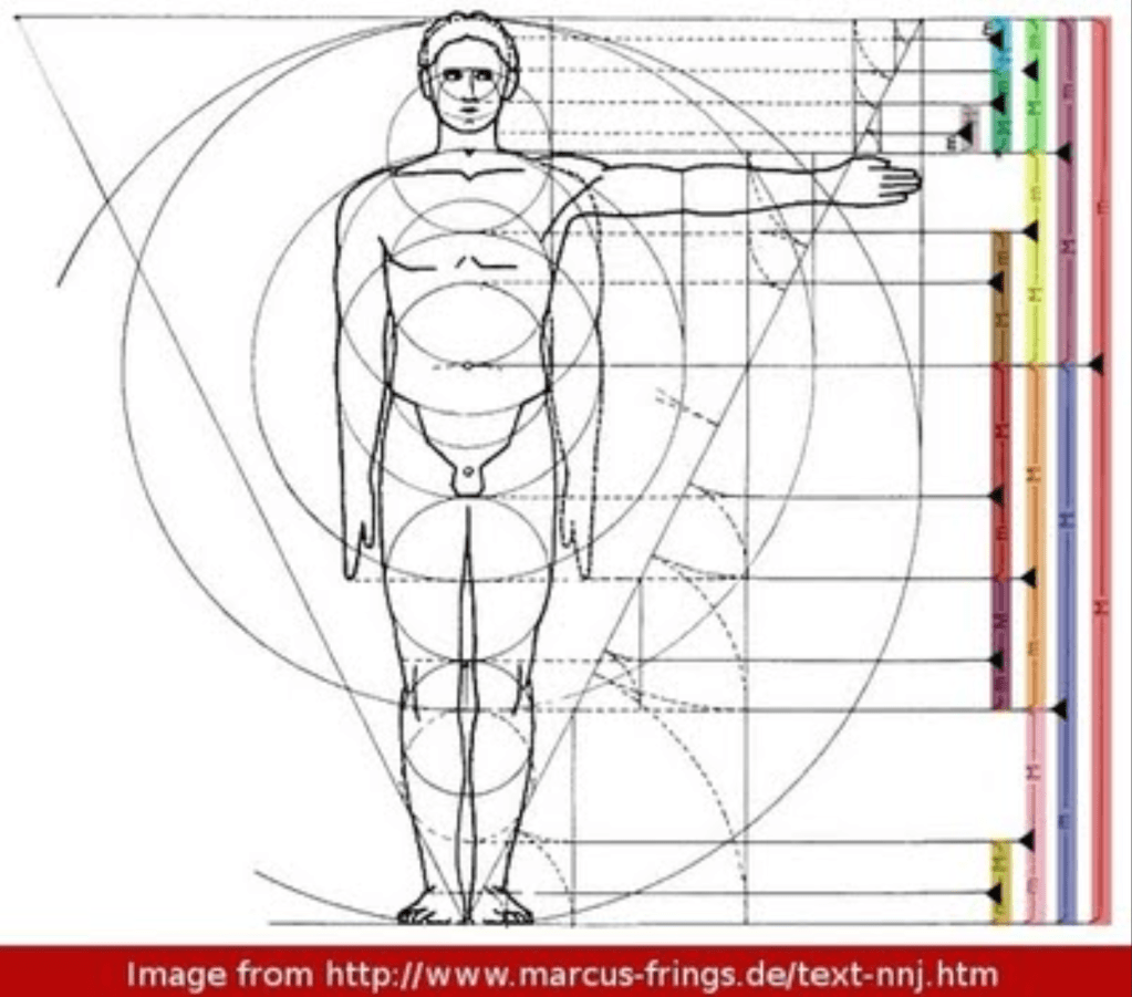
If ever there was a magic number that encoded the mysteries of the universe, then surely it must be the golden mean. It seems to pop up everywhere. In flowers and hurricanes. In pine cones and sea shells. In architecture and infinite sums. In telescoping cascades of golden rectangles in the human figure.
Fig. 1. The golden mean can be found in numerous ratios of the measurements of the human body.
It also rears its head in the world of chaos theory, governing how a twisting dumbbell rotor transitions from regular motion to chaotic motion when it is tapped gently at a regular period.
The Golden Ratio
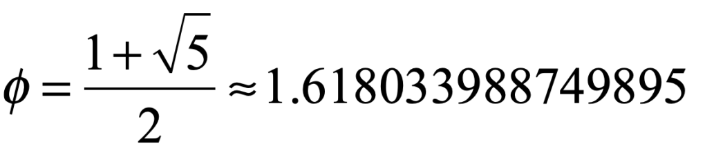
The Golden ratio can be defined in many ways, but its most common expression is given by
Among its many marvelous properties, one is that it is the hardest number to approximate with a ratio of small integers. For instance, the ratio 89/55 is a number that is as close as one part in ten thousand to the golden mean but it is hardly a ratio of small integers. This result may seem obscure, but there is a systematic way to find the ratios of integers that approximate an irrational number. This is known as continued fractions.
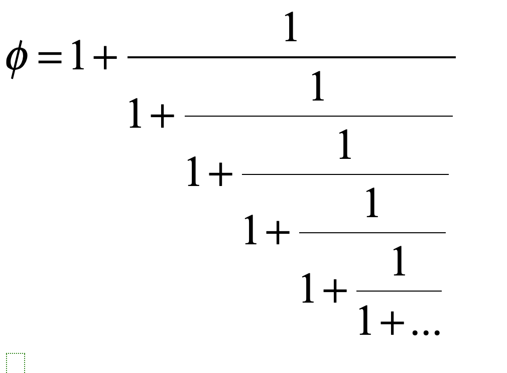
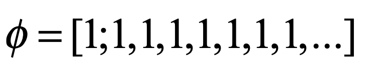
The continued fraction for the golden mean has an especially simple repeating form
also written as
This continued fraction has the slowest convergence for its continued fraction of any other number. Hence, the Golden Ratio can be considered, using this criterion, to be the most irrational number of all, and it governs the last straw of order as chaos emerges from a surprisingly simple map.
The Kicked Rigid Rotor
The rigid rotator (the simple dumbbell) is one of the iconic systems in physics. It is a classic object in the study of rotational dynamics, showing up in Lagrangian formulations as well as Euler’s equations. It is also a classic system in elementary quantum mechanics, illustrating the quantization of angular momentum. In the current setting (Hamiltonian chaos), it is an example of a periodically perturbed system that displays beautiful phenomena.
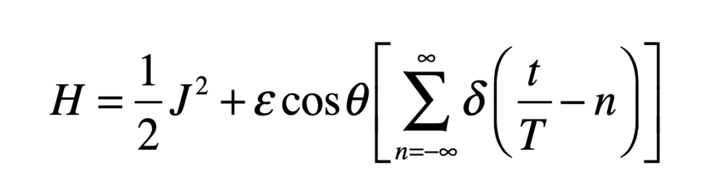
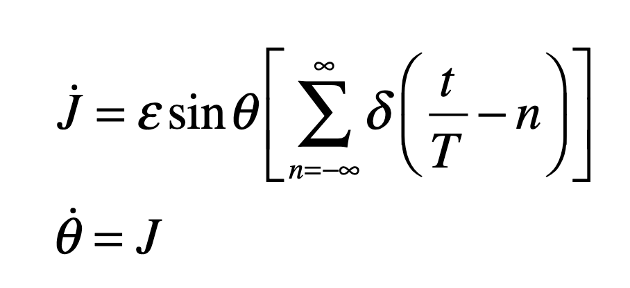
In chaos theory, the relationship between a continuous dynamical system and its discrete map is sometimes difficult to identify. However, a discrete map arises naturally from a randomly kicked dumbbell rotator. The system has an angular momentum J and a physical angle θ. The strength of the angular momentum kick is given by the perturbation parameter ε, and the torque of the kick is a function of the physical angle θ. The kicked rotator has the Hamiltonian
where the kicks are evenly timed with period T. The perturbation parameter ε can be large. The perturbation amplitude and sign depend on the instantaneous angle θ. The equations of motion from Hamilton’s equations are
The values for J and θ just before the nth successive kick are Jn and qn, respectively. Because the evaluation of the variables occurs at the period T, these discrete observations represent the values of a Poincaré section.
The Chirikov Twist Map
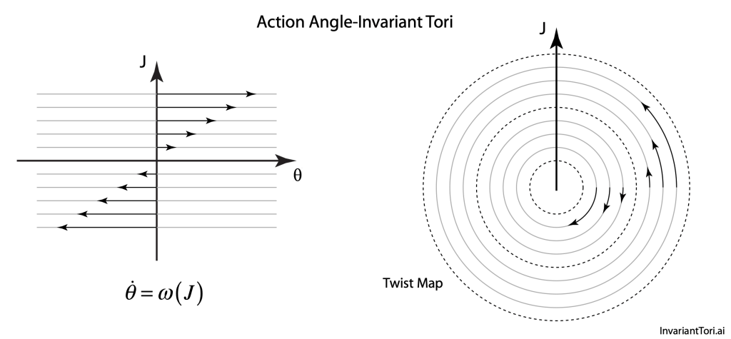
The phase space (in action-angle coordinates) of the rigid rotator is particularly attractive for applications because it is simply a linear flow that has increasing velocities with increasing action J. In action-angle representation, it is a twist map, where circles outside the radius for J = 0 twist in one direction but inside that radius they twist in the opposite direction. David Birkhoff showed in 1913, while proving Poincaré’s last geometric theorem, that a simple periodic perturbation of this system creates a set of closed trajectories (around an elliptical point) and a set of open trajectories (around a hyperbolic point).
Fig. 2. The action-angle phase space of a rigid rotator, plus the associated twist map.
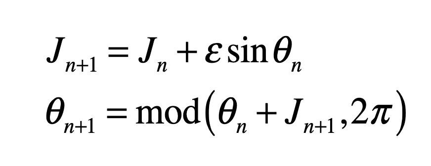
The rotator dynamics are continuous between each kick, leading to the discrete map (known as the Standard Map or the Chirikov Map)
in which the rotator is “strobed”, or observed, at regular periods of 2π. When ε = 0, the orbits on the (θ, J) plane are simply horizontal lines—the rotator spins with regular motion at a speed determined by J.
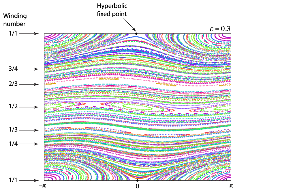
As the strength of the kick ε increases from zero, the Poicaré-Birkhoff theorem kicks in, and a first “island chain” appears with a single elliptical point paired with a single hyperbolic point. Then at larger values of ε new island chains appear, first with two islands, then with three, as in the figure below with ε = 0.3. Orbits that produce two islands are in a 2:1 resonance, and with three islands are in either a 3:1 or a 3:2 resonance. With increasing ε, more and more island chains open up, representing higher resonances.
Fig. 3 Chirikov map for ε = 0.3. The 1/1, 1/2 and 1/3 (2/3) island chains have opened with a primary hyperbolic point on the 1/1 resonance.
Each resonance is associated with a ratio of small integers: 1/2; 2/3; 3/4; 4/5 and beyond. These are the natural harmonics of the system. As the integers get larger, the ratios begin to approximate irrational numbers.
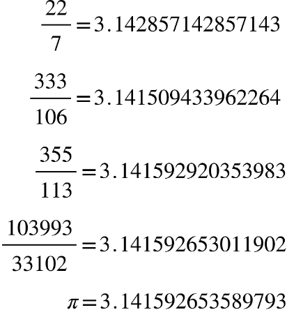
For instance, the number pi is approximated to increasing accuracy by the sequence of ratios:
Fig. Successive convergents of the irrational number pi.
These are called convergents and are obtained by taking more terms in the continued fraction representation of pi.
One of the fundamental findings of the theory of resonances in Hamiltonian systems is the decreasing “weight” of resonances associated with ratios of larger integers. Therefore, the 1:2 resonance is by far the most robust, the first to spring into existence, and it survives up to extremely strong perturbations. The 1:3 resonance is also relativety robust, but already the 1:4 and 1:5 resonances are more sensitive to perturbation and break up into island chains under moderate perturbation. Clearly the 22:7 ratio would not be sensitive nor the 333:106 resonance. These orbits would resist breaking up. Furthermore, once a resonance turns into an island chain, it creates hyperbolic points that can nucleate chaotic trajectories.
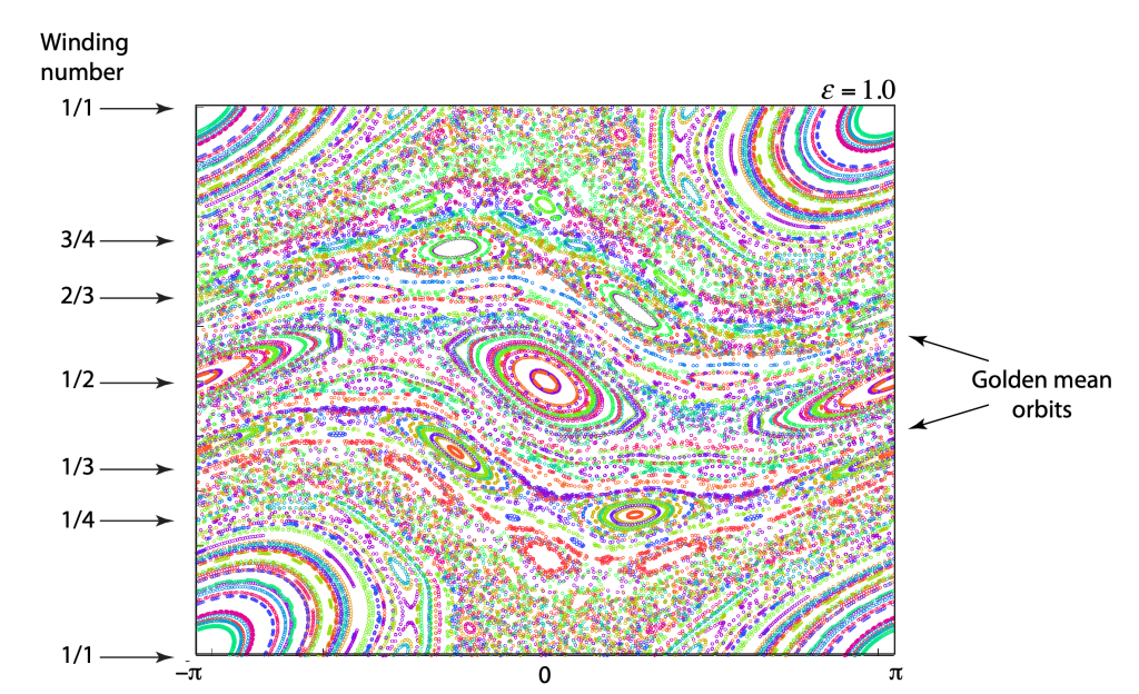
An example of the twist map at strong perturbation ε = 1.0 is shown in Fig. 4. There are numerous island chains. It is easy to find the 1:2 through the 1:7 resonances, but beyond that it is much more difficult to find these rational resonance. Furthermore, there are significant regions of chaotic trajectories associated with the hyperbolic points of the 1:2, 1:3, 1:4 and 1:5 resonances.
Fig. 4. The Standard map at ε = 1.0 slightly above the threshold for the dissolution of the Golde-Mean-Orbit.
In the midst of the island chains and the chaos, there are still continuous (open) orbits that span the phase space without breaks. These are the most irrational numbers–numbers like the golden mean. These are the last orbits to break up. The critical threshold for the breakup of the golden-mean orbit is ε = 0.971. The plot in Fig. 4 is just above that threshold.
All of this behavior of the Standard Map follows from KAM theory, developed by Kolmogorov, Arnold and Moser in the early 1960’s. Although the standard map is specific to the tapped spinning disk, the results and behavior are very general for a wide class of two-dimensional Hamiltonian dynamical systems.
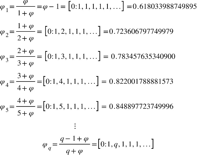
Adiabatic Following: Orbits of the Noble Means
The golden mean is not the only “slowest convergent” among irrational numbers. There are an entire class of irrational numbers whose continued fractions terminate with an infinite series of “1”s. These are known as the “Noble Means”. Examples are:
where the sequence, as q increases to infinity, converges on unity asymptotically among the set of irrationals with the slowest convergents.
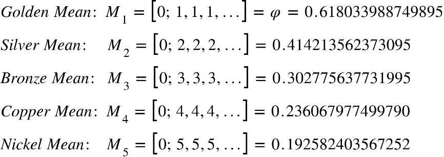
There are also the so-called “Metallic Means”, beginning with Gold and moving to Silver, Bronze, Copper, and Nickel. These are:
The challenge for numerical simulations is to find the orbits associated with these Metallic Means for large perturbation parameters ε. One cannot simply pick an initial condition for the Standard Map equal to a Metallic Mean, because at large perturbation, all the orbits have already shifted from their zero-perturbation values.
One of the most important principles in classical mechanics is the concept of adiabatic invariance. All the most common conservation laws of introductory physics–conservation of energy, momentum, and angular momentum–are consequences of adiabatic invariance. Indeed, the phase space of the rigid rotator is ideal for tracking adiabatic invariance because the J-value is the adiabatic invariant. In the numerical simulation, one begins with ε = 0, chooses an initial condition J = φn, and iterates the map as ε slowly increases.
This is shown in the following YouTube video. You will see five special orbits evolve as the perturbation is slowly increased. These are M1 (red), M2 (blue), M3 (green) and two resonances 3:1 (cyan) and 4:1 (magenta). The resonances are expected to break into island chains at relativity low perturbation ε, which is confirmed in the video.
Fig. 5 YouTube video of the Standard Map and special orbits as the perturbation slowly (adiabatically) increases.
Interestingly, the silver mean breaks into a 5:1 island chain around the same perturbation level. This is because the Silver Mean equals 0.414 which approaches 8/5 at moderate perturbation. Therefore, the Silver Mean orbit is “captured” by a 1:5 resonance and remains stable up to very large perturbations approaching ε = 1. The Bronze Mean is captured relativity early into the 1:1 resonance island.
D. D. Nolte, Introduction to Modern Dynamics, 2nd ed. (Oxford University Press, 2019) Link
This Post is Based on Simulations from Chapter 5 of IMD, 2nd edition
This Blog Post is a Companion to the undergraduate physics textbook Modern Dynamics: Chaos, Networks, Space and Time, 2nd ed. (Oxford, 2019) introducing Lagrangians and Hamiltonians, chaos theory, complex systems, synchronization, neural networks, econophysics and Special and General Relativity to Junior and Senior physics majors.
Chaos seems to rule our world. Weather events, natural disasters, economic volatility, empire building—all these contribute to the complexities that buffet our lives. It is no wonder that ancient man attributed the chaos to the gods or to the fates, infinitely far from anything we can comprehend as cause and effect. Yet there is a balm to soothe our wounds from the slings of life—Chaos Theory—if not to solve our problems, then at least to understand them.
Chaos Theory is the theory of complex systems governed by multiple factors that produce complicated outputs. The power of the theory is its ability recognize when the complicated outputs are not “random”, no matter how complicated they are, but are in fact determined by the inputs. Furthermore, chaos theory finds structures and patterns within the output—like the fractal structures known as “strange attractors”. These patterns not only are not random, but they tell us about the internal mechanics of the system, and they tell us where to look “on average” for the system behavior.
In other words, chaos theory tames the chaos, and we no longer need to blame gods or the fates.
Henri Poincare (1889)
The first glimpse of the inner workings of chaos was made by accident when Henri Poincaré responded to a mathematics competition held in honor of the King of Sweden. The challenge was to prove whether the solar system was absolutely stable, or whether there was a danger that one day the Earth would be flung from its orbit. Poincaré had already been thinking about the stability of dynamical systems so he wrote up his solution to the challenge and sent it in, believing that he had indeed proven that the solar system was stable.
His entry to the competition was the most convincing, so he was awarded the prize and instructed to submit the manuscript for publication. The paper was already at the printers and coming off the presses when Poincaré was asked by the competition organizer to check one last part of the proof which one of the reviewer’s had questioned relating to homoclinic orbits.
Fig. 1 A homoclinic orbit is an orbit in phase space that intersects itself.
To Poincaré’s horror, as he checked his results against the reviewer’s comments, he found that he had made a fundamental error, and in fact the solar system would never be stable. The problem that he had overlooked had to do with the way that orbits can cross above or below each other on successive passes, leading to a tangle of orbital trajectories that crisscrossed each other in a fine mesh. This is known as the “homoclinic tangle”: it was the first glimpse that deterministic systems could lead to unpredictable results. Most importantly, he had developed the first mathematical tools that would be needed to analyze chaotic systems—such as the Poincaré section—but nearly half a century would pass before these tools would be picked up again.
Poincaré paid out of his own pocket for the first printing to be destroyed and for the corrected version of his manuscript to be printed in its place [1]. No-one but the competition organizers and reviewers ever saw his first version. Yet it was when he was correcting his mistake that he stumbled on chaos for the first time, which is what posterity remembers him for. This little episode in the history of physics went undiscovered for a century before being brought to light by Barrow-Green in her 1997 book Poincaré and the Three Body Problem [2].
Fig. 2 Henri Poincaré’s homoclinic tangle from the Standard Map. (The picture on the right is the Poincaré crater on the moon). For more details, see my blog on Poincaré and his Homoclinic Tangle.
Cartwight and Littlewood (1945)
During World War II, self-oscillations and nonlinear dynamics became strategic topics for the war effort in England. High-power magnetrons were driving long-range radar, keeping Britain alert to Luftwaffe bombing raids, and the tricky dynamics of these oscillators could be represented as a driven van der Pol oscillator. These oscillators had been studied in the 1920’s by the Dutch physicist Balthasar van der Pol (1889–1959) when he was completing his PhD thesis at the University of Utrecht on the topic of radio transmission through ionized gases. van der Pol had built a short-wave triode oscillator to perform experiments on radio diffraction to compare with his theoretical calculations of radio transmission. Van der Pol’s triode oscillator was an engineering feat that produced the shortest wavelengths of the day, making van der Pol intimately familiar with the operation of the oscillator, and he proposed a general form of differential equation for the triode oscillator.
Fig. 3 Driven van der Pol oscillator equation.
Research on the radar magnetron led to theoretical work on driven nonlinear oscillators, including the discovery that a driven van der Pol oscillator could break up into wild and intermittent patterns. This “bad” behavior of the oscillator circuit (bad for radar applications) was the first discovery of chaotic behavior in man-made circuits.
These irregular properties of the driven van der Pol equation were studied by Mary- Lucy Cartwright (1990–1998) (the first woman to be elected a fellow of the Royal Society) and John Littlewood (1885–1977) at Cambridge who showed that the coexistence of two periodic solutions implied that discontinuously recurrent motion—in today’s parlance, chaos— could result, which was clearly undesirable for radar applications. The work of Cartwright and Littlewood [3] later inspired the work by Levinson and Smale as they introduced the field of nonlinear dynamics.
Fig. 4 Mary Cartwright
Andrey Kolmogorov (1954)
The passing of the Russian dictator Joseph Stalin provided a long-needed opening for Soviet scientists to travel again to international conferences where they could meet with their western colleagues to exchange ideas. Four Russian mathematicians were allowed to attend the 1954 International Congress of Mathematics (ICM) held in Amsterdam, the Netherlands. One of those was Andrey Nikolaevich Kolmogorov (1903 – 1987) who was asked to give the closing plenary speech. Despite the isolation of Russia during the Soviet years before World War II and later during the Cold War, Kolmogorov was internationally renowned as one of the greatest mathematicians of his day.
By 1954, Kolmogorov’s interests had spread into topics in topology, turbulence and logic, but no one was prepared for the topic of his plenary lecture at the ICM in Amsterdam. Kolmogorov spoke on the dusty old topic of Hamiltonian mechanics. He even apologized at the start for speaking on such an old topic when everyone had expected him to speak on probability theory. Yet, in the length of only half an hour he laid out a bold and brilliant outline to a proof that the three-body problem had an infinity of stable orbits. Furthermore, these stable orbits provided impenetrable barriers to the diffusion of chaotic motion across the full phase space of the mechanical system. The crucial consequences of this short talk were lost on almost everyone who attended as they walked away after the lecture, but Kolmogorov had discovered a deep lattice structure that constrained the chaotic dynamics of the solar system.
Kolmogorov’s approach used a result from number theory that provides a measure of how close an irrational number is to a rational one. This is an important question for orbital dynamics, because whenever the ratio of two orbital periods is a ratio of integers, especially when the integers are small, then the two bodies will be in a state of resonance, which was the fundamental source of chaos in Poincaré’s stability analysis of the three-body problem. After Komogorov had boldly presented his results at the ICM of 1954 [4], what remained was the necessary mathematical proof of Kolmogorov’s daring conjecture. This would be provided by one of his students, V. I. Arnold, a decade later. But before the mathematicians could settle the issue, an atmospheric scientist, using one of the first electronic computers, rediscovered Poincaré’s tangle, this time in a simplified model of the atmosphere.
Edward Lorenz (1963)
In 1960, with the help of a friend at MIT, the atmospheric scientist Edward Lorenz purchased a Royal McBee LGP-30 tabletop computer to make calculation of a simplified model he had derived for the weather. The McBee used 113 of the latest miniature vacuum tubes and also had 1450 of the new solid-state diodes made of semiconductors rather than tubes, which helped reduce the size further, as well as reducing heat generation. The McBee had a clock rate of 120 kHz and operated on 31-bit numbers with a 15 kB memory. Under full load it used 1500 Watts of power to run. But even with a computer in hand, the atmospheric equations needed to be simplified to make the calculations tractable. Lorenz simplified the number of atmospheric equations down to twelve, and he began programming his Royal McBee.
Progress was good, and by 1961, he had completed a large initial numerical study. One day, as he was testing his results, he decided to save time by starting the computations midway by using mid-point results from a previous run as initial conditions. He typed in the three-digit numbers from a paper printout and went down the hall for a cup of coffee. When he returned, he looked at the printout of the twelve variables and was disappointed to find that they were not related to the previous full-time run. He immediately suspected a faulty vacuum tube, as often happened. But as he looked closer at the numbers, he realized that, at first, they tracked very well with the original run, but then began to diverge more and more rapidly until they lost all connection with the first-run numbers. The internal numbers of the McBee had a precision of 6 decimal points, but the printer only printed three to save time and paper. His initial conditions were correct to a part in a thousand, but this small error was magnified exponentially as the solution progressed. When he printed out the full six digits (the resolution limit for the machine), and used these as initial conditions, the original trajectory returned. There was no mistake. The McBee was working perfectly.
At this point, Lorenz recalled that he “became rather excited”. He was looking at a complete breakdown of predictability in atmospheric science. If radically different behavior arose from the smallest errors, then no measurements would ever be accurate enough to be useful for long-range forecasting. At a more fundamental level, this was a break with a long-standing tradition in science and engineering that clung to the belief that small differences produced small effects. What Lorenz had discovered, instead, was that the deterministic solution to his 12 equations was exponentially sensitive to initial conditions (known today as SIC).
The more Lorenz became familiar with the behavior of his equations, the more he felt that the 12-dimensional trajectories had a repeatable shape. He tried to visualize this shape, to get a sense of its character, but it is difficult to visualize things in twelve dimensions, and progress was slow, so he simplified his equations even further to three variables that could be represented in a three-dimensional graph [5].
Fig. 5 Two-dimensional projection of the three-dimensional Lorenz Butterfly.
V. I. Arnold (1964)
Meanwhile, back in Moscow, an energetic and creative young mathematics student knocked on Kolmogorov’s door looking for an advisor for his undergraduate thesis. The youth was Vladimir Igorevich Arnold (1937 – 2010), who showed promise, so Kolmogorov took him on as his advisee. They worked on the surprisingly complex properties of the mapping of a circle onto itself, which Arnold filed as his dissertation in 1959. The circle map holds close similarities with the periodic orbits of the planets, and this problem led Arnold down a path that drew tantalizingly close to Kolmogorov’s conjecture on Hamiltonian stability. Arnold continued in his PhD with Kolmogorov, solving Hilbert’s 13th problem by showing that every function of n variables can be represented by continuous functions of a single variable. Arnold was appointed as an assistant in the Faculty of Mechanics and Mathematics at Moscow State University.
Arnold’s habilitation topic was Kolmogorov’s conjecture, and his approach used the same circle map that had played an important role in solving Hilbert’s 13th problem. Kolmogorov neither encouraged nor discouraged Arnold to tackle his conjecture. Arnold was led to it independently by the similarity of the stability problem with the problem of continuous functions. In reference to his shift to this new topic for his habilitation, Arnold stated “The mysterious interrelations between different branches of mathematics with seemingly no connections are still an enigma for me.” [6]
Arnold began with the problem of attracting and repelling fixed points in the circle map and made a fundamental connection to the theory of invariant properties of action-angle variables . These provided a key element in the proof of Kolmogorov’s conjecture. In late 1961, Arnold submitted his results to the leading Soviet physics journal—which promptly rejected it because he used forbidden terms for the journal, such as “theorem” and “proof”, and he had used obscure terminology that would confuse their usual physicist readership, terminology such as “Lesbesgue measure”, “invariant tori” and “Diophantine conditions”. Arnold withdrew the paper.
Arnold later incorporated an approach pioneered by Jurgen Moser [7] and published a definitive article on the problem of small divisors in 1963 [8]. The combined work of Kolmogorov, Arnold and Moser had finally established the stability of irrational orbits in the three-body problem, the most irrational and hence most stable orbit having the frequency of the golden mean. The term “KAM theory”, using the first initials of the three theorists, was coined in 1968 by B. V. Chirikov, who also introduced in 1969 what has become known as the Chirikov map (also known as the Standard map ) that reduced the abstract circle maps of Arnold and Moser to simple iterated functions that any student can program easily on a computer to explore KAM invariant tori and the onset of Hamiltonian chaos, as in Fig. 1 [9].
Fig. 6 The Chirikov Standard Map when the last stable orbits are about to dissolve for ε = 0.97.
Sephen Smale (1967)
Stephen Smale was at the end of a post-graduate fellowship from the National Science Foundation when he went to Rio to work with Mauricio Peixoto. Smale and Peixoto had met in Princeton in 1960 where Peixoto was working with Solomon Lefschetz (1884 – 1972) who had an interest in oscillators that sustained their oscillations in the absence of a periodic force. For instance, a pendulum clock driven by the steady force of a hanging weight is a self-sustained oscillator. Lefschetz was building on work by the Russian Aleksandr A. Andronov (1901 – 1952) who worked in the secret science city of Gorky in the 1930’s on nonlinear self-oscillations using Poincaré’s first return map. The map converted the continuous trajectories of dynamical systems into discrete numbers, simplifying problems of feedback and control.
The central question of mechanical control systems, even self-oscillating systems, was how to attain stability. By combining approaches of Poincaré and Lyapunov, as well as developing their own techniques, the Gorky school became world leaders in the theory and applications of nonlinear oscillations. Andronov published a seminal textbook in 1937 The Theory of Oscillations with his colleagues Vitt and Khaykin, and Lefschetz had obtained and translated the book into English in 1947, introducing it to the West. When Peixoto returned to Rio, his interest in nonlinear oscillations captured the imagination of Smale even though his main mathematical focus was on problems of topology. On the beach in Rio, Smale had an idea that topology could help prove whether systems had a finite number of periodic points. Peixoto had already proven this for two dimensions, but Smale wanted to find a more general proof for any number of dimensions.
Norman Levinson (1912 – 1975) at MIT became aware of Smale’s interests and sent off a letter to Rio in which he suggested that Smale should look at Levinson’s work on the triode self-oscillator (a van der Pol oscillator), as well as the work of Cartwright and Littlewood who had discovered quasi-periodic behavior hidden within the equations. Smale was puzzled but intrigued by Levinson’s paper that had no drawings or visualization aids, so he started scribbling curves on paper that bent back upon themselves in ways suggested by the van der Pol dynamics. During a visit to Berkeley later that year, he presented his preliminary work, and a colleague suggested that the curves looked like strips that were being stretched and bent into a horseshoe.
Smale latched onto this idea, realizing that the strips were being successively stretched and folded under the repeated transformation of the dynamical equations. Furthermore, because dynamics can move forward in time as well as backwards, there was a sister set of horseshoes that were crossing the original set at right angles. As the dynamics proceeded, these two sets of horseshoes were repeatedly stretched and folded across each other, creating an infinite latticework of intersections that had the properties of the Cantor set. Here was solid proof that Smale’s original conjecture was wrong—the dynamics had an infinite number of periodicities, and they were nested in self-similar patterns in a latticework of points that map out a Cantor-like set of points. In the two-dimensional case, shown in the figure, the fractal dimension of this lattice is D = ln4/ln3 = 1.26, somewhere in dimensionality between a line and a plane. Smale’s infinitely nested set of periodic points was the same tangle of points that Poincaré had noticed while he was correcting his King Otto Prize manuscript. Smale, using modern principles of topology, was finally able to put rigorous mathematical structure to Poincaré’s homoclinic tangle. Coincidentally, Poincaré had launched the modern field of topology, so in a sense he sowed the seeds to the solution to his own problem.
Fig. 7 The horseshoe takes regions of phase space and stretches and folds them over and over to create a lattice of overlapping trajectories.
Ruelle and Takens (1971)
The onset of turbulence was an iconic problem in nonlinear physics with a long history and a long list of famous researchers studying it. As far back as the Renaissance, Leonardo da Vinci had made detailed studies of water cascades, sketching whorls upon whorls in charcoal in his famous notebooks. Heisenberg, oddly, wrote his PhD dissertation on the topic of turbulence even while he was inventing quantum mechanics on the side. Kolmogorov in the 1940’s applied his probabilistic theories to turbulence, and this statistical approach dominated most studies up to the time when David Ruelle and Floris Takens published a paper in 1971 that took a nonlinear dynamics approach to the problem rather than statistical, identifying strange attractors in the nonlinear dynamical Navier-Stokes equations [10]. This paper coined the phrase “strange attractor”. One of the distinct characteristics of their approach was the identification of a bifurcation cascade. A single bifurcation means a sudden splitting of an orbit when a parameter is changed slightly. In contrast, a bifurcation cascade was not just a single Hopf bifurcation, as seen in earlier nonlinear models, but was a succession of Hopf bifurcations that doubled the period each time, so that period-two attractors became period-four attractors, then period-eight and so on, coming fast and faster, until full chaos emerged. A few years later Gollub and Swinney experimentally verified the cascade route to turbulence , publishing their results in 1975 [11].
Fig. 8 Bifurcation cascade of the logistic map.
Feigenbaum (1978)
In 1976, computers were not common research tools, although hand-held calculators now were. One of the most famous of this era was the Hewlett-Packard HP-65, and Feigenbaum pushed it to its limits. He was particularly interested in the bifurcation cascade of the logistic map [12]—the way that bifurcations piled on top of bifurcations in a forking structure that showed increasing detail at increasingly fine scales. Feigenbaum was, after all, a high-energy theorist and had overlapped at Cornell with Kenneth Wilson when he was completing his seminal work on the renormalization group approach to scaling phenomena. Feigenbaum recognized a strong similarity between the bifurcation cascade and the ideas of real-space renormalization where smaller and smaller boxes were used to divide up space.
One of the key steps in the renormalization procedure was the need to identify a ratio of the sizes of smaller structures to larger structures. Feigenbaum began by studying how the bifurcations depended on the increasing growth rate. He calculated the threshold values rm for each of the bifurcations, and then took the ratios of the intervals, comparing the previous interval (rm-1 – rm-2) to the next interval (rm – rm-1). This procedure is like the well-known method to calculate the golden ratio = 1.61803 from the Fibonacci series, and Feigenbaum might have expected the golden ratio to emerge from his analysis of the logistic map. After all, the golden ratio has a scary habit of showing up in physics, just like in the KAM theory. However, as the bifurcation index m increased in Feigenbaum’s study, this ratio settled down to a limiting value of 4.66920. Then he did what anyone would do with an unfamiliar number that emerges from a physical calculation—he tried to see if it was a combination of other fundamental numbers, like pi and Euler’s constant e, and even the golden ratio. But none of these worked. He had found a new number that had universal application to chaos theory [13].
Fig. 9 The ratio of the limits of successive cascades leads to a new universal number (the Feigenbaum number).
Gleick (1987)
By the mid-1980’s, chaos theory was seeping in to a broadening range of research topics that seemed to span the full breadth of science, from biology to astrophysics, from mechanics to chemistry. A particularly active group of chaos practitioners were J. Doyn Farmer, James Crutchfield, Norman Packard and Robert Shaw who founded the Dynamical Systems Collective at the University of California, Santa Cruz. One of the important outcomes of their work was a method to reconstruct the state space of a complex system using only its representative time series [14]. Their work helped proliferate the techniques of chaos theory into the mainstream. Many who started using these techniques were only vaguely aware of its long history until the science writer James Gleick wrote a best-selling history of the subject that brought chaos theory to the forefront of popular science [15]. And the rest, as they say, is history.
By David D. Nolte, April 3, 2024
References
[1] Poincaré, H. and D. L. Goroff (1993). New methods of celestial mechanics. Edited and introduced by Daniel L. Goroff. New York, American Institute of Physics.
[2] J. Barrow-Green, Poincaré and the three body problem (London Mathematical Society, 1997).
[3] Cartwright,M.L.andJ.E.Littlewood(1945).“Onthenon-lineardifferential equation of the second order. I. The equation y′′ − k(1 – yˆ2)y′ + y = bλk cos(λt + a), k large.” Journal of the London Mathematical Society 20: 180–9. Discussed in Aubin, D. and A. D. Dalmedico (2002). “Writing the History of Dynamical Systems and Chaos: Longue DurÈe and Revolution, Disciplines and Cultures.” Historia Mathematica, 29: 273.
[4] Kolmogorov, A. N., (1954). “On conservation of conditionally periodic motions for a small change in Hamilton’s function.,” Dokl. Akad. Nauk SSSR (N.S.), 98: 527–30.
[5] Lorenz, E. N. (1963). “Deterministic Nonperiodic Flow.” Journal of the Atmo- spheric Sciences 20(2): 130–41.
[6] Arnold,V.I.(1997).“From superpositions to KAM theory,”VladimirIgorevich Arnold. Selected, 60: 727–40.
[7] Moser, J. (1962). “On Invariant Curves of Area-Preserving Mappings of an Annulus.,” Nachr. Akad. Wiss. Göttingen Math.-Phys, Kl. II, 1–20.
[8] Arnold, V. I. (1963). “Small denominators and problems of the stability of motion in classical and celestial mechanics (in Russian),” Usp. Mat. Nauk., 18: 91–192,; Arnold, V. I. (1964). “Instability of Dynamical Systems with Many Degrees of Freedom.” Doklady Akademii Nauk Sssr 156(1): 9.
[9] Chirikov, B. V. (1969). Research concerning the theory of nonlinear resonance andstochasticity. Institute of Nuclear Physics, Novosibirsk. 4. Note: The Standard Map Jn+1 =Jn +εsinθn θn+1 =θn +Jn+1 is plotted in Fig. 3.31 in Nolte, Introduction to Modern Dynamics (2015) on p. 139. For small perturbation ε, two fixed points appear along the line J = 0 corresponding to p/q = 1: one is an elliptical point (with surrounding small orbits) and the other is a hyperbolic point where chaotic behavior is first observed. With increasing perturbation, q elliptical points and q hyperbolic points emerge for orbits with winding numbers p/q with small denominators (1/2, 1/3, 2/3 etc.). Other orbits with larger q are warped by the increasing perturbation but are not chaotic. These orbits reside on invariant tori, known as the KAM tori, that do not disintegrate into chaos at small perturbation. The set of KAM tori is a Cantor-like set with non- zero measure, ensuring that stable behavior can survive in the presence of perturbations, such as perturbation of the Earth’s orbit around the Sun by Jupiter. However, with increasing perturbation, orbits with successively larger values of q disintegrate into chaos. The last orbits to survive in the Standard Map are the golden mean orbits with p/q = φ–1 and p/q = 2–φ. The critical value of the perturbation required for the golden mean orbits to disintegrate into chaos is surprisingly large at εc = 0.97.
[10] Ruelle,D. and F.Takens (1971).“OntheNatureofTurbulence.”Communications in Mathematical Physics 20(3): 167–92.
[11] Gollub, J. P. and H. L. Swinney (1975). “Onset of Turbulence in a Rotating Fluid.” Physical Review Letters, 35(14): 927–30.
[12] May, R. M. (1976). “Simple Mathematical-Models with very complicated Dynamics.” Nature, 261(5560): 459–67.
[13] M. J. Feigenbaum, “Quantitative Universality for a Class of Nnon-linear Transformations,” Journal of Statistical Physics 19, 25-52 (1978).
[14] Packard, N.; Crutchfield, J. P.; Farmer, J. Doyne; Shaw, R. S. (1980). “Geometry from a Time Series”. Physical Review Letters. 45 (9): 712–716.
Fractals, those telescoping self-similar filigree meshes that marry mathematics and art, have become so mainstream, that they are even mentioned in the theme song of Disney’s 2013 mega-hit, Frozen.
My power flurries through the air into the ground My soul is spiraling in frozen fractals all around And one thought crystallizes like an icy blast I’m never going back, the past is in the past
Let it Go, by Idina Menzel (Frozen, Disney 2013)
But not all fractals are cut from the same cloth. Some are thin and some are fat. The thin ones are the ones we know best, adorning the cover of books and magazines. But the fat ones may be more common and may play important roles, such as in the stability of celestial orbits in a many-planet neighborhood, or in the stability and structure of Saturn’s rings.
To get a handle on fat fractals, we will start with a familiar thin one, the zero-measure Cantor set.
The Zero-Measure Cantor Set
The famous one-third Cantor set is often the first fractal that you encounter in any introduction to fractals. (See my blog on a short history of fractals.) It lives on a one-dimensional line, and its iterative construction is intuitive and simple.
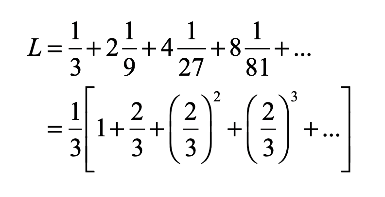
Start with a long thin bar of unit length. Then remove the middle third, leaving the endpoints. This leaves two identical bars of one-third length each. Next, remove the open middle third of each of these, again leaving the endpoints, leaving behind section pairs of one-nineth length. Then repeat ad infinitum. The points of the line that remain–all those segment endpoints–are the Cantor set.
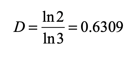
Fig. 1 Construction of the 1/3 Cantor set by removing 1/3 segments at each level, and leaving the endpoints of each segment. The resulting set is a dust of points with a fractal dimension D = ln(2)/ln(3) = 0.6309.
The Cantor set has a fractal dimension that is easily calculated by noting that at each stage there are two elements (N = 2) that divided by three in size (b = 3). The fractal dimension is then
It is easy to prove that the collection of points of the Cantor set have no length because all of the length was removed.
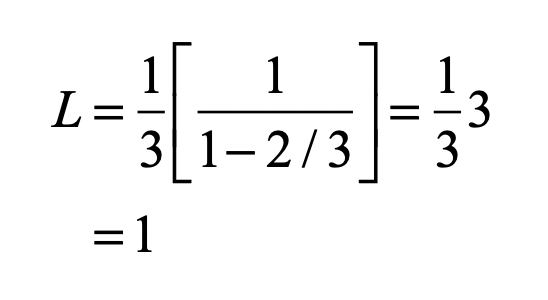
For instance, at the first level, one third of the length was removed. At the second level, two segments of one-nineth length were removed. At the third level, four segments of one-twenty-sevength length were removed, and so on. Mathematically, this is
The infinite series in the brackets is a binomial series with the simple solution
Therefore, all the length has been removed, and none is left to the Cantor set, which is simply a collection of all the endpoints of all the segments that were removed.
The Cantor set is said to have a Lebesgue measure of zero. It behaves as a dust of isolated points.
A close relative of the Cantor set is the Sierpinski Carpet which is the two-dimensional analog. It begins with a square of unit side, then the middle third is removed (one nineth of the three-by-three array of square of one-third side), and so on.
Fig. 2 A regular Sierpinski Carpet with fractal dimension D = ln(8)/ln(3) = 1.8928.
The resulting Sierpinski Carpet has zero Lebesgue measure, just like the Cantor dust, because all the area has been removed.
There are also random Sierpinski Carpets as the sub-squares are removed from random locations.
Fig. 3 A random Sierpinski Carpet with fractal dimension D = ln(8)/ln(3) = 1.8928.
These fractals are “thin”, so-called because they are dusts with zero measure.
But the construction was constructed just so, such that the sum over all the removed sub-lengths summed to unity. What if less material had been taken at each step? What happens?
Fat Fractals
Instead of taking one-third of the original length, take instead one-fourth. But keep the one-third scaling level-to-level, as for the original Cantor Set.
Fig. 4 A “fat” Cantor fractal constructed by removing 1/4 of a segment at each level instead of 1/3.
The total length removed is
Therefore, three fourths of the length was removed, leaving behind one fourth of the material. Not only that, but the material left behind is contiguous—solid lengths. At each level, a little bit of the original bar remains, and still remains at the next level and the next. Therefore, it is said to have a Lebesgue measure of unity. This construction leads to a “fat” fractal.
Fig. 5 Fat Cantor fractal showing the original Cantor 1/3 set (in black) and the extra contiguous segments (in red) that give the set a Lebesgue measure equal to one.
Looking at Fig. 5, it is clear that the original Cantor dust is still present as the black segments interspersed among the red parts of the bar that are contiguous. But when two sets are added that have different “dimensions”, then the combined set has the larger dimension of the two, which is one-dimensional in this case. The fat Cantor set is one dimensional. One can still study its scaling properties, leading to another type of dimension known as an exterior measure [1], but where do such fat fractals occur? Why do they matter?
One answer is that they lie within the oddly named “Arnold Tongues” that arise in the study of synchronization and resonance connected to the stability of the solar system and the safety of its inhabitants.
Arnold Tongues
The study of synchronization explores and explains how two or more non-identical oscillators can lock themselves onto a common shared oscillation. For two systems to synchronize requires autonomous oscillators (like planetary orbits) with a period-dependent interaction (like gravity). Such interactions are “resonant” when the periods of the two orbits are integer ratios of each other, like 1:2 or 2:3. Such resonances ensure that there is a periodic forcing caused by the interaction that is some multiple of the orbital period. Think of tapping a rotating bicycle wheel twice per cycle or three times per cycle. Even if you are a little off in your timing, you can lock the tire rotation rate to a multiple of your tapping frequency. But if you are too far off on your timing, then the wheel will turn independently of your tapping.
Because rational ratios of integers are plentiful, there can be an intricate interplay between locked frequencies and unlocked frequencies. When the rotation rate is close to a resonance, then the wheel can frequency-lock to the tapping. Plotting the regions where the wheel synchronizes or not as a function of the frequency ratio and also as a function of the strength of the tapping leads to one of the iconic images of nonlinear dynamics: the Arnold tongue diagram.
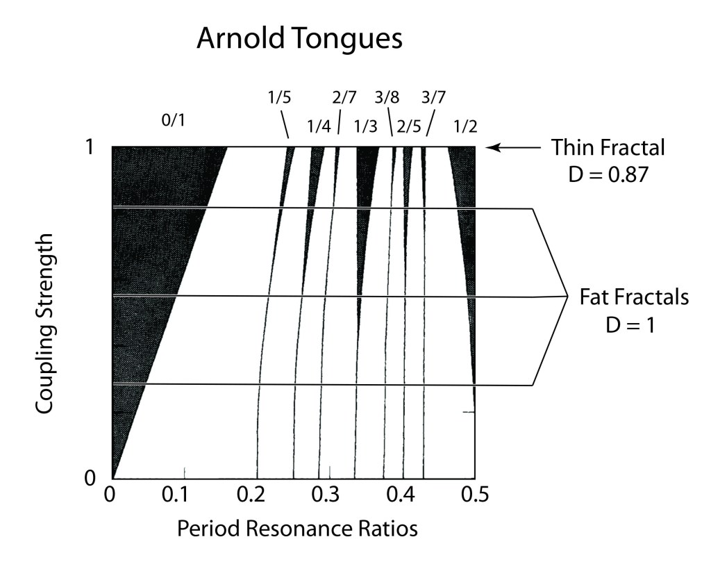
Fig. 6 Arnold tongue diagram, showing the regions of frequency locking (black) at rational resonances as a function of coupling strength. At unity coupling strength, the set outside frequency-locked regions is fractal with D = 0.87. For all smaller coupling, a set along a horizontal is a fat fractal with topological dimension D = 1. The white regions are “ergodic”, as the phase of the oscillator runs through all possible values.
The Arnold tongues in Fig. 6 are the frequency locked regions (black) as a function of frequency ratio and coupling strength g. The black regions correspond to rational ratios of frequencies. For g = 1, the set outside frequency-locked regions (the white regions are “ergodic”, as the phase of the oscillator runs through all possible values) is a thin fractal with D = 0.87. For g < 1, the sets outside the frequency locked regions along a horizontal (at constant g) are fat fractals with topological dimension D = 1. For fat fractals, the fractal dimension is irrelevant, and another scaling exponent takes on central importance.
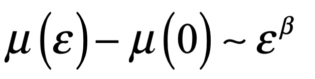
The Lebesgue measure μ of the ergodic regions (the regions that are not frequency locked) is a function of the coupling strength varying from μ = 1 at g = 0 to μ = 0 at g = 1. When the pattern is coarse-grained at a scale ε, then the scaling of a fat fractal is
where β is the scaling exponent that characterizes the fat fractal.
From numerical studies [2] there is strong evidence that β = 2/3 for the fat fractals of Arnold Tongues.
The Rings of Saturn
Arnold Tongues arise in KAM theory on the stability of the solar system (See my blog on KAM and how number theory protects us from the chaos of the cosmos). Fortunately, Jupiter is the largest perturbation to Earth’s orbit, but its influence, while non-zero, is not enough to seriously affect our stability. However, there is a part of the solar system where rational resonances are not only large but dominant: Saturn’s rings.
Saturn’s rings are composed of dust and ice particles that orbit Saturn with a range of orbital periods. When one of these periods is a rational fraction of the orbital period of a moon, then a resonance condition is satisfied. Saturn has many moons, producing highly corrugated patterns in Saturn’s rings at rational resonances of the periods.
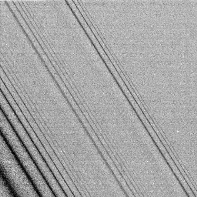
Fig. 7 A close up of Saturn’s rings shows a highly detailed set of bands. Particles at a given radius have a given period (set by Kepler’s third law). When the period of dust particles in the ring are an integer ratio of the period of a “shepherd moon”, then a resonance can drive density rings. [See image reference.]
The moons Janus and Epithemeus share an orbit around Saturn in a rare 1:1 resonance in which they swap positions every four years. Their combined gravity excites density ripples in Saturn’s rings, photographed by the Cassini spacecraft and shown in Fig. 8.
Fig. 8 Cassini spacecraft photograph of density ripples in Saturns rings caused by orbital resonance with the pair of moons Janus and Epithemeus.
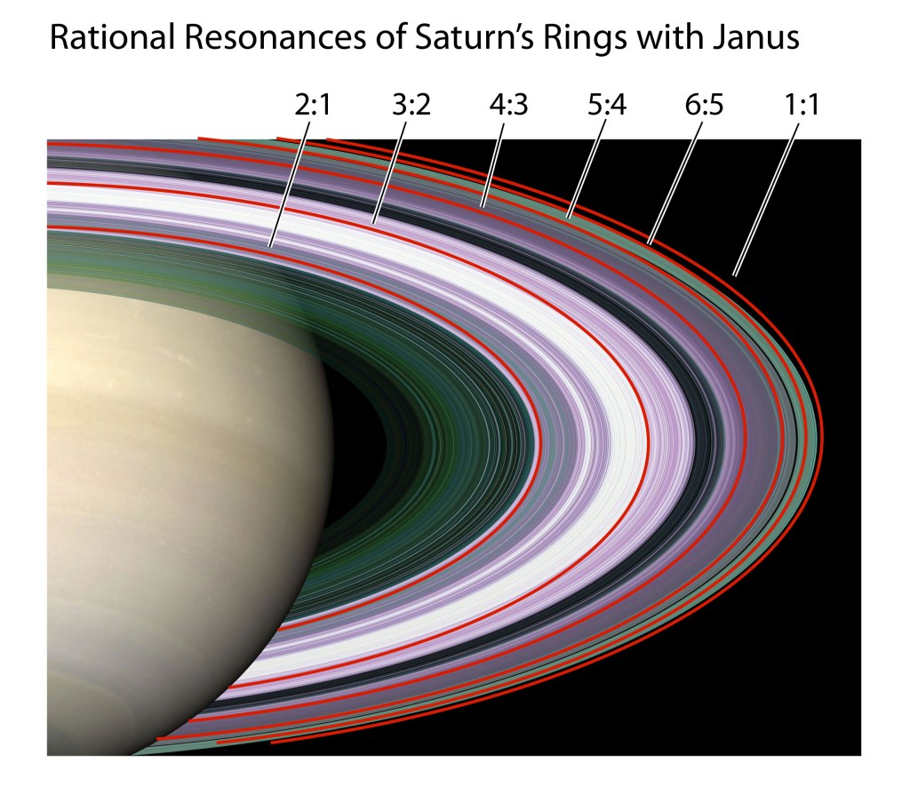
One Canadian astronomy group converted the resonances of the moon Janus into a musical score to commenorate Cassini’s final dive into the planet Saturn in 2017. The Janus resonances are shown in Fig. 9 against the pattern of Saturn’s rings.
Fig. 7 Rational resonances for subrings of Saturn relative to its moon Janus.
Saturn’s rings, orbital resonances, Arnold tongues and fat fractals provide a beautiful example of the power of dynamics to create structure, and the primary role that structure plays in deciphering the physics of complex systems.
By David D. Nolte, Nov. 28, 2023
References:
[1] C. Grebogi, S. W. McDonald, E. Ott, and J. A. Yorke, “EXTERIOR DIMENSION OF FAT FRACTALS,” Physics Letters A 110, 1-4 (1985).
[2] R. E. Ecke, J. D. Farmer, and D. K. Umberger, “Scaling of the Arnold tongues,” Nonlinearity 2, 175-196 (1989).
Read more in Books by David Nolte at Oxford University Press
We are exceedingly fortunate that the Earth lies in the Goldilocks zone. This zone is the range of orbital radii of a planet around its sun for which water can exist in a liquid state. Water is the universal solvent, and it may be a prerequisite for the evolution of life. If we were too close to the sun, water would evaporate as steam. And if we are too far, then it would be locked in perpetual ice. As it is, the Earth has had wild swings in its surface temperature. There was once a time, more than 650 million years ago, when the entire Earth’s surface froze over. Fortunately, the liquid oceans remained liquid, and life that already existed on Earth was able to persist long enough to get to the Cambrian explosion. Conversely, Venus may once have had liquid oceans and maybe even nascent life, but too much carbon dioxide turned the planet into an oven and boiled away its water (a fate that may await our own Earth if we aren’t careful). What has saved us so far is the stability of our orbit, our steady distance from the Sun that keeps our water liquid and life flourishing. Yet it did not have to be this way.
The regions of regular motion associated with irrational numbers act as if they were a barrier, restricting the range of chaotic orbits and protecting other nearby orbits from the chaos.
Our solar system is a many-body problem. It consists of three large gravitating bodies (Sun, Jupiter, Saturn) and several minor ones (such as Earth). Jupiter does influence our orbit, and if it were only a few times more massive than it actually is, then our orbit would become chaotic, varying in distance from the sun in unpredictable ways. And if Jupiter were only about 20 times bigger than is actually is, there is a possibility that it would perturb the Earth’s orbit so strongly that it could eject the Earth from the solar system entirely, sending us flying through interstellar space, where we would slowly cool until we became a permanent ice ball. What can protect us from this terrifying fate? What keeps our orbit stable despite the fact that we inhabit a many-body solar system? The answer is number theory!
The Most Irrational Number
What is the most irrational
number you can think of?
Is it: pi = 3.1415926535897932384626433 ?
Or Euler’s constant: e = 2.7182818284590452353602874 ?
How about: sqrt(3) = 1.73205080756887729352744634 ?
These are all perfectly good irrational numbers. But how do you choose the “most irrational” number? The answer is fairly simple. The most irrational number is the one that is least well approximated by a ratio of integers. For instance, it is possible to get close to pi through the ratio 22/7 = 3.1428 which differs from pi by only 4 parts in ten thousand. Or Euler’s constant 87/32 = 2.7188 differs from e by only 2 parts in ten thousand. Yet 87 and 32 are much bigger than 22 and 7, so it may be said that e is more irrational than pi, because it takes ratios of larger integers to get a good approximation. So is there a “most irrational” number? The answer is yes. The Golden Ratio.
The Golden ratio can be defined in many ways, but its most common expression is given by
It is the hardest number to approximate with a ratio of small integers. For instance, to get a number that is as close as one part in ten thousand to the golden mean takes the ratio 89/55. This result may seem obscure, but there is a systematic way to find the ratios of integers that approximate an irrational number. This is known as a convergent from continued fractions.
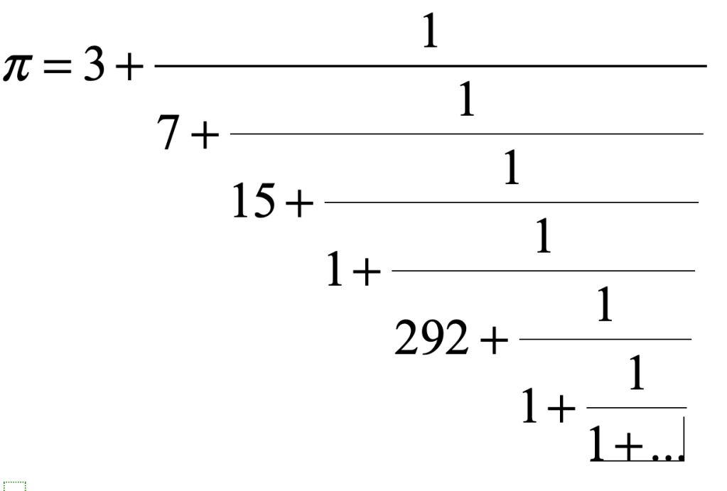
Continued fractions were invented by John Wallis in 1695, introduced in his book Opera Mathematica. The continued fraction for pi is
An alternate form of displaying this continued fraction is with the expression
The irrational character of pi is captured by the seemingly random integers in this string. However, there can be regular structure in irrational numbers. For instance, a different continued fraction for pi is
that has a surprisingly simple repeating pattern.
The continued fraction for the golden mean has an especially simple repeating form
or
This continued fraction has the slowest convergence for its continued fraction of any other number. Hence, the Golden Ratio can be considered, using this criterion, to be the most irrational number.
If the Golden Ratio is the most irrational number, how does that save us from the chaos of the cosmos? The answer to this question is KAM!
Kolmogorov, Arnold and Moser: (KAM) Theory
KAM is an acronym made from the first initials of three towering mathematicians of the 20th century: Andrey Kolmogorov (1903 – 1987), his student Vladimir Arnold (1937 – 2010), and Jürgen Moser (1928 – 1999).
In 1954, Kolmogorov, considered to be the greatest living mathematician at that time, was invited to give the plenary lecture at a mathematics conference. To the surprise of the conference organizers, he chose to talk on what seemed like a very mundane topic: the question of the stability of the solar system. This had been the topic which Poincaré had attempted to solve in 1890 when he first stumbled on chaotic dynamics. The question had remained open, but the general consensus was that the many-body nature of the solar system made it intrinsically unstable, even for only three bodies.
Against all expectations, Kolmogorov proposed that despite the general chaotic behavior of the three–body problem, there could be “islands of stability” which were protected from chaos, allowing some orbits to remain regular even while other nearby orbits were highly chaotic. He even outlined an approach to a proof of his conjecture, though he had not carried it through to completion.
The proof of Kolmogorov’s conjecture was supplied over the next 10 years through the work of the German mathematician Jürgen Moser and by Kolmogorov’s former student Vladimir Arnold. The proof hinged on the successive ratios of integers that approximate irrational numbers. With this work KAM showed that indeed some orbits are actually protected from neighboring chaos by relying on the irrationality of the ratio of orbital periods.
Resonant Ratios
Let’s go back to the simple model of our solar system that consists of only three bodies: the Sun, Jupiter and Earth. The period of Jupiter’s orbit is 11.86 years, but instead, if it were exactly 12 years, then its period would be in a 12:1 ratio with the Earth’s period. This ratio of integers is called a “resonance”, although in this case it is fairly mismatched. But if this ratio were a ratio of small integers like 5:3, then it means that Jupiter would travel around the sun 5 times in 15 years while the Earth went around 3 times. And every 15 years, the two planets would align. This kind of resonance with ratios of small integers creates a strong gravitational perturbation that alters the orbit of the smaller planet. If the perturbation is strong enough, it could disrupt the Earth’s orbit, creating a chaotic path that might ultimately eject the Earth completely from the solar system.
What KAM discovered is that as the resonance ratio becomes a ratio of large integers, like 87:32, then the planets have a hard time aligning, and the perturbation remains small. A surprising part of this theory is that a nearby orbital ratio might be 5:2 = 1.5, which is only a little different than 87:32 = 1.7. Yet the 5:2 resonance can produce strong chaos, while the 87:32 resonance is almost immune. This way, it is possible to have both chaotic orbits and regular orbits coexisting in the same dynamical system. An irrational orbital ratio protects the regular orbits from chaos. The next question is, how irrational does the orbital ratio need to be to guarantee safety?
You probably already guessed the answer to this question–the answer must be the Golden Ratio. If this is indeed the most irrational number, then it cannot be approximated very well with ratios of small integers, and this is indeed the case. In a three-body system, the most stable orbital ratio would be a ratio of 1.618034. But the more general question of what is “irrational enough” for an orbit to be stable against a given perturbation is much harder to answer. This is the field of Diophantine Analysis, which addresses other questions as well, such as Fermat’s Last Theorem.
KAM Twist Map
The dynamics of three-body systems are hard to visualize directly, so there are tricks that help bring the problem into perspective. The first trick, invented by Henri Poincaré, is called the first return map (or the Poincaré section). This is a way of reducing the dimensionality of the problem by one dimension. But for three bodies, even if they are all in a plane, this still can be complicated. Another trick, called the restricted three-body problem, is to assume that there are two large masses and a third small mass. This way, the dynamics of the two-body system is unaffected by the small mass, so all we need to do is focus on the dynamics of the small body. This brings the dynamics down to two dimensions (the position and momentum of the third body), which is very convenient for visualization, but the dynamics still need solutions to differential equations. So the final trick is to replace the differential equations with simple difference equations that are solved iteratively.
A simple discrete iterative map that captures the essential behavior of the three-body problem begins with action-angle variables that are coupled through a perturbation. Variations on this model have several names: the Twist Map, the Chirikov Map and the Standard Map. The essential mapping is
where J is an action variable (like angular momentum) paired with the angle variable. Initial conditions for the action and the angle are selected, and then all later values are obtained by iteration. The perturbation parameter is given by ε. If ε = 0 then all orbits are perfectly regular and circular. But as the perturbation increases, the open orbits split up into chains of closed (periodic) orbits. As the perturbation increases further, chaotic behavior emerges. The situation for ε = 0.9 is shown in the figure below. There are many regular periodic orbits as well as open orbits. Yet there are simultaneously regions of chaotic behavior. This figure shows an intermediate case where regular orbits can coexist with chaotic ones. The key is the orbital period ratio. For orbital ratios that are sufficiently irrational, the orbits remain open and regular. Bur for orbital ratios that are ratios of small integers, the perturbation is strong enough to drive the dynamics into chaos.
Arnold Twist Map (also known as a Chirikov map) for ε = 0.9 showing the chaos that has emerged at the hyperbolic point, but there are still open orbits that are surprisingly circular (unperturbed) despite the presence of strongly chaotic orbits nearby.
#!/usr/bin/env python3
# -*- coding: utf-8 -*-
"""
Created on Wed Oct. 2, 2019
@author: nolte
"""
import numpy as np
from scipy import integrate
from matplotlib import pyplot as plt
plt.close('all')

eps = 0.9

np.random.seed(2)
plt.figure(1)
for eloop in range(0,50):

    rlast = np.pi*(1.5*np.random.random()-0.5)
    thlast = 2*np.pi*np.random.random()

    orbit = np.int(200*(rlast+np.pi/2))
    rplot = np.zeros(shape=(orbit,))
    thetaplot = np.zeros(shape=(orbit,))
    x = np.zeros(shape=(orbit,))
    y = np.zeros(shape=(orbit,))
    for loop in range(0,orbit):
        rnew = rlast + eps*np.sin(thlast)
        thnew = np.mod(thlast+rnew,2*np.pi)

        rplot[loop] = rnew
        thetaplot[loop] = np.mod(thnew-np.pi,2*np.pi) - np.pi

        rlast = rnew
        thlast = thnew

        x[loop] = (rnew+np.pi+0.25)*np.cos(thnew)
        y[loop] = (rnew+np.pi+0.25)*np.sin(thnew)

    plt.plot(x,y,'o',ms=1)

plt.savefig('StandMapTwist')
The twist map for three values of ε are shown in the figure below. For ε = 0.2, most orbits are open, with one elliptic point and its associated hyperbolic point. At ε = 0.9 the periodic elliptic point is still stable, but the hyperbolic point has generated a region of chaotic orbits. There is still a remnant open orbit that is associated with an orbital period ratio at the Golden Ratio. However, by ε = 0.97, even this most stable orbit has broken up into a chain of closed orbits as the chaotic regions expand.
Twist map for three levels of perturbation.
Safety in Numbers
In our solar system, governed by gravitational attractions, the square of the orbital period increases as the cube of the average radius (Kepler’s third law). Consider the restricted three-body problem of the Sun and Jupiter with the Earth as the third body. If we analyze the stability of the Earth’s orbit as a function of distance from the Sun, the orbital ratio relative to Jupiter would change smoothly. Near our current position, it would be in a 12:1 resonance, but as we moved farther from the Sun, this ratio would decrease. When the orbital period ratio is sufficiently irrational, then the orbit would be immune to Jupiter’s pull. But as the orbital ratio approaches ratios of integers, the effect gets larger. Close enough to Jupiter there would be a succession of radii that had regular motion separated by regions of chaotic motion. The regions of regular motion associated with irrational numbers act as if they were a barrier, restricting the range of chaotic orbits and protecting more distant orbits from the chaos. In this way numbers, rational versus irrational, protect us from the chaos of our own solar system.
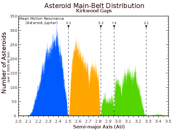
A dramatic demonstration of the orbital resonance effect can be seen with the asteroid belt. The many small bodies act as probes of the orbital resonances. The repetitive tug of Jupiter opens gaps in the distribution of asteroid radii, with major gaps, called Kirkwood Gaps, opening at orbital ratios of 3:1, 5:2, 7:3 and 2:1. These gaps are the radii where chaotic behavior occurs, while the regions in between are stable. Most asteroids spend most of their time in the stable regions, because chaotic motion tends to sweep them out of the regions of resonance. This mechanism for the Kirkwood gaps is the same physics that produces gaps in the rings of Saturn at resonances with the many moons of Saturn.
The gaps in the asteroid distributions caused by orbital resonances with Jupiter. Ref. Wikipedia
For a more detailed mathematical description of the KAM theory, see Chapter 5, Hamiltonian Chaos, in Introduction to Modern Dynamics, 2nd edition (Oxford University Press, 2019).
See also:
Dumas, H. S., The KAM Story: A friendly introduction to the content, history and significance of Classical Kolmogorov-Arnold-Moser Theory. World Scientific: 2014.
Arnold, V. I., From superpositions to KAM theory. Vladimir Igorevich Arnold. Selected Papers 1997, PHASIS, 60, 727–740.
The Physics of Life, the Universe and Everything:
Read more about the history of chaos theory in Galileo Unbound from Oxford University Press (2018)