Climate Change Physics 101

When our son was ten years old, he came home from a town fair in Battleground, Indiana, with an unwanted pet—a goldfish in a plastic bag.  The family rushed out to buy a fish bowl and food and plopped the golden-red animal into it.  In three days, it was dead!

It turns out that you can’t just put a gold fish in a fish bowl.  When it metabolizes its food and expels its waste, it builds up toxic levels of ammonia unless you add filters or plants or treat the water with chemicals.  In the end, the goldfish died because it was asphyxiated by its own pee.

It’s a basic rule—don’t pee in your own fish bowl.

The same can be said for humans living on the surface of our planet.  Polluting the atmosphere with our wastes cannot be a good idea.  In the end it will kill us.  The atmosphere may look vast—the fish bowl was a big one—but it is shocking how thin it is.

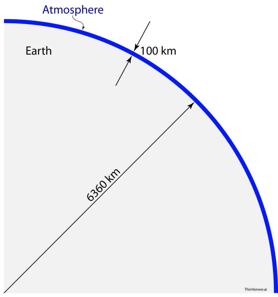
Turn on your Apple TV, click on the screen saver, and you are skimming over our planet on the dark side of the Earth. Then you see a thin blue line extending over the limb of the dark disc.  Hold!  That thin blue line!  That is our atmosphere! Is it really so thin?

When you look upwards on a clear sunny day, the atmosphere seems like it goes on forever.  It doesn’t.  It is a thin veneer on the surface of the Earth barely one percent of the Earth’s radius.  The Earth’s atmosphere is frighteningly thin. 

Fig. 1  A thin veneer of atmosphere paints the surface of the Earth.  The radius of the Earth is 6360 km, and the thickness of the atmosphere is 100 km, which is a bit above 1 percent of the radius.

Consider Mars.  It’s half the size of Earth, yet it cannot hold on to an atmosphere even 1/100th the thickness of ours.  When Mars first formed, it had an atmosphere not unlike our own, but through the eons its atmosphere has wafted away irretrievably into space.

An atmosphere is a precious fragile thing for a planet.  It gives life and it gives protection.  It separates us from the deathly cold of space, holding heat like a blanket.  That heat has served us well over the eons, allowing water to stay liquid and allowing life to arise on Earth.  But too much of a good thing is not a good thing.

Common Sense

If the fluid you are bathed in gives you life, then don’t mess with it.  Don’t run your car in the garage while you are working in it.  Don’t use a charcoal stove in an enclosed space.  Don’t dump carbon dioxide into the atmosphere because it also is an enclosed space.

At the end of winter, as the warm spring days get warmer, you take the winter blanket off your bed because blankets hold in heat.  The thicker the blanket, the more heat it holds in.  Common sense tells you to reduce the thickness of the blanket if you don’t want to get too warm.  Carbon dioxide in the atmosphere acts like a blanket.  If we don’t want the Earth to get too warm, then we need to limit the thickness of the blanket.

Without getting into the details of any climate change model, common sense already tells us what we should do.  Keep the atmosphere clean and stable (Don’t’ pee in our fishbowl) and limit the amount of carbon dioxide we put into it (Don’t let the blanket get too thick).

Some Atmospheric Facts

Here are some facts about the atmosphere, about the effect humans have on it, and about the climate:

Fact 1.  Humans have increased the amount of carbon dioxide in the atmosphere by 45% since 1850 (the beginning of the industrial age) and by 30% since just 1960.

Fact 2.  Carbon dioxide in the atmosphere prevents some of the heat absorbed from the Sun to re-radiate out to space.  More carbon dioxide stores more heat.

Fact 3.  Heat added to the Earth’s atmosphere increases its temperature.  This is a law of physics.

Fact 4.  The Earth’s average temperature has risen by 1.2 degrees Celsius since 1850 and 0.8 degrees of that has been just since 1960, so the effect is accelerating.

These facts are indisputable.  They hold true regardless of whether there is a Republican or a Democrat in the White House or in control of Congress.

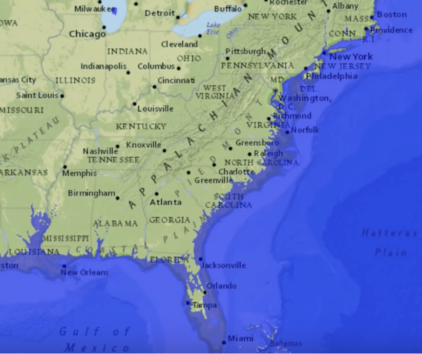
There is another interesting observation which is not so direct, but may hold a harbinger for the distant future: The last time the Earth was 3 degrees Celsius warmer than it is today was during the Pliocene when the sea level was tens of meters higher.  If that sea level were to occur today, all of Delaware, most of Florida, half of Louisiana and the entire east coast of the US would be under water, including Houston, Miami, New Orleans, Philadelphia and New York City.  There are many reasons why this may not be an immediate worry. The distribution of water and ice now is different than in the Pliocene, and the effect of warming on the ice sheets and water levels could take centuries. Within this century, the amount of sea level rise is likely to be only about 1 meter, but accelerating after that.

Fig. 2  The east coast of the USA for a sea level 30 meters higher than today.  All of Delaware, half of Louisiana, and most of Florida are under water. Reasonable projections show only a 1 meter sea level rise by 2100, but accelerating after that. From https://www.youtube.com/watch?v=G2x1bonLJFA

Balance and Feedback

It is relatively easy to create a “rule-of-thumb” model for the Earth’s climate (see Ref. [2]).  This model is not accurate, but it qualitatively captures the basic effects of climate change and is a good way to get an intuitive feeling for how the Earth responds to changes, like changes in CO2 or to the amount of ice cover.  It can also provide semi-quantitative results, so that relative importance of various processes or perturbations can be understood.

The model is a simple energy balance statement:  In equilibrium, as much energy flows into the Earth system as out.

This statement is both simple and immediately understandable.  But then the work starts as we need to pin down how much energy is flowing in and how much is flowing out.  The energy flowing in comes from the sun, and the energy flowing out comes from thermal radiation into space. 

We also need to separate the Earth system into two components: the surface and the atmosphere.  These are two very different things that have two different average temperatures.  In addition, the atmosphere transmits sunlight to the surface, unless clouds reflect it back into space.  And the Earth radiates thermally into space, unless clouds or carbon dioxide layers reflect it back to the surface.

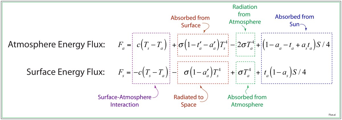
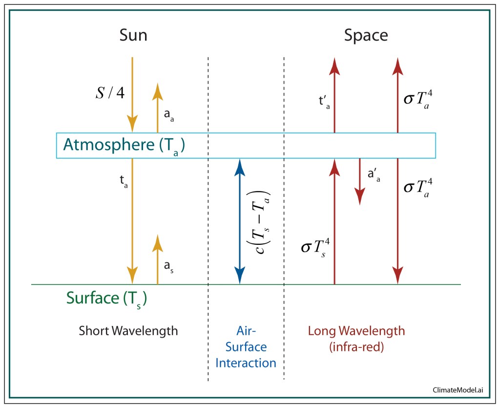
The energy fluxes are shown in the diagram in Fig. 3 for the 4-component system: Sun, Surface, Atmosphere, and Space. The light from the sun, mostly in the visible range of the spectrum, is partially absorbed by the atmosphere and partially transmitted and reflected. The transmitted portion is partially absorbed and partially reflected by the surface. The heat of the Earth is radiated at long wavelengths to the atmosphere, where it is partially transmitted out into space, but also partially reflected by the fraction a’a which is the blanket effect. In addition, the atmosphere itself radiates in equal parts to the surface and into outer space. On top of all of these radiative processes, there is also non-radiative convective interaction between the atmosphere and the surface.

Fig. 3 Energy flux model for a simple climate model with four interacting systems: the Sun, the Atmosphere, the Earth and Outer Space.

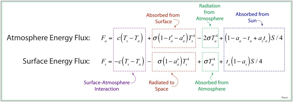
These processes are captured by two energy flux equations, one for the atmosphere and one for the surface, in Fig. 4. The individual contributions from Fig. 3 are annotated in each case. In equilibrium, each flux equals zero, which can then be used to solve for the two unknowns: Ts0 and Ta0: the surface and atmosphere temperatures.

Fig. 4 Energy-balance model of the Earth’s atmosphere for a simple climate approximation.

After the equilibrium temperatures Ts0 and Ta0 are found, they go into a set of dynamic response equations that governs how deviations in the temperatures relax back to the equilibrium values. These relaxation equations are

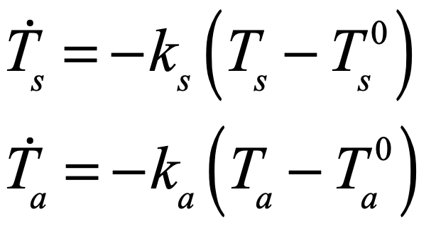
where ks and ka are the relaxation rates for the surface and atmosphere. These can be quite slow, in the range of a century. For illustration, we can take ks = 1/75 years and ka = 1/25 years. The equilibrium temperatures for the surface and atmosphere differ by about 50 degrees Celsius, with Ts = 289 K and Ta = 248 K. These are rough averages over the entire planet. The solar constant is S = 1.36×10³ W/m2, the Stefan-Boltzman constant is σ = 5.67×10⁻⁸ W/m2/K4, and the convective interaction constant is c = 2.5 W m-2 K-1. Other parameters are given in Table I.

Short WavelengthLong Wavelength
as = 0.11
ts = 0.53t’a = 0.06
aa = 0.30a’a = 0.31

The relaxation equations are in the standard form of a mathematical “flow” (see Ref. [1]) and the solutions are plotted as a phase-space portrait in Fig. 5 as a video of the flow as the parameters in Table I shift because of the addition of greenhouse gases to the atmosphere. The video runs from the year 1850 (the dawn of the industrial age) through to the year 2060 about 40 years from now.

Fig. 5 Video of the phase space flow of the Surface-Atmosphere system for increasing year. The flow vectors and flow lines are the relaxation to equilibrium for temperature deviations. The change in equilibrium over the years is from increasing blanket effects in the atmosphere caused by greenhouse gases.

The scariest part of the video is how fast it accelerates. From 1850 to 1950 there is almost no change, but then it accelerates, faster and faster, reflecting the time-lag in temperature rise in response to increased greenhouse gases.

What if the Models are Wrong?  Russian Roulette

Now come the caveats.

This model is just for teaching purposes, not for any realistic modeling of climate change. It captures the basic physics, and it provides a semi-quantitative set of parameters that leads to roughly accurate current temperatures. But of course, the biggest elephant in the room is that it averages over the entire planet, which is a very crude approximation.

It does get the basic facts correct, though, showing an alarming trend in the rise in average temperatures with the temperature rising by 3 degrees by 2060.

The professionals in this business have computer models that are orders of magnitude more more accurate than this one. To understand the details of the real climate models, one needs to go to appropriate resources, like this NOAA link, this NASA link, this national climate assessment link, and this government portal link, among many others.

One of the frequent questions that is asked is: What if these models are wrong? What if global warming isn’t as bad as these models say? The answer is simple: If they are wrong, then the worst case is that life goes on. If they are right, then in the worst case life on this planet may end.

It’s like playing Russian Roulette. If just one of the cylinders on the revolver has a live bullet, do you want to pull the trigger?

Matlab Code

function flowatmos.m

mov_flag = 1;
if mov_flag == 1
    moviename = 'atmostmp';
    aviobj = VideoWriter(moviename,'MPEG-4');
    aviobj.FrameRate = 12;
    open(aviobj);
end

Solar = 1.36e3;		% Solar constant outside atmosphere [J/sec/m2]
sig = 5.67e-8;		% Stefan-Boltzman constant [W/m2/K4]

% 1st-order model of Earth + Atmosphere

ta = 0.53;			% (0.53)transmissivity of air
tpa0 = 0.06;			% (0.06)primes are for thermal radiation
as0 = 0.11;			% (0.11)
aa0 = 0.30;			% (0.30)
apa0 = 0.31;        % (0.31)
c = 2.5;               % W/m2/K

xrange = [287 293];
yrange = [247 251];

rngx = xrange(2) - xrange(1);
rngy = yrange(2) - yrange(1);

[X,Y] = meshgrid(xrange(1):0.05:xrange(2), yrange(1):0.05:yrange(2));

smallarrow = 1;
Delta0 = 0.0000009;
for tloop =1:80
    
    Delta = Delta0*(exp((tloop-1)/8)-1);   % This Delta is exponential, but should become more linear over time
    date = floor(1850 + (tloop-1)*(2060-1850)/79);
    
    [x,y] = f5(X,Y);
    
    clf
    hold off
    eps = 0.002;
    for xloop = 1:11
        xs = xrange(1) +(xloop-1)*rngx/10 + eps;
        for yloop = 1:11
            ys = yrange(1) +(yloop-1)*rngy/10 + eps;
            
            streamline(X,Y,x,y,xs,ys)
            
        end
    end
    hold on
    [XQ,YQ] = meshgrid(xrange(1):1:xrange(2),yrange(1):1:yrange(2));
    smallarrow = 1;
    [xq,yq] = f5(XQ,YQ);
    quiver(XQ,YQ,xq,yq,.2,'r','filled')
    hold off
    
    axis([xrange(1) xrange(2) yrange(1) yrange(2)])
    set(gcf,'Color','White')
    
    fun = @root2d;
    x0 = [0 -40];
    x = fsolve(fun,x0);
    
    Ts = x(1) + 288
    Ta = x(2) + 288
    
    hold on
    rectangle('Position',[Ts-0.05 Ta-0.05 0.1 0.1],'Curvature',[1 1],'FaceColor',[1 0 0],'EdgeColor','k','LineWidth',2)
    
    posTs(tloop) = Ts;
    posTa(tloop) = Ta;
    
    plot(posTs,posTa,'k','LineWidth',2);
    hold off
    
    text(287.5,250.5,strcat('Date = ',num2str(date)),'FontSize',24)
    box on
    xlabel('Surface Temperature (oC)','FontSize',24)
    ylabel('Atmosphere Temperature (oC)','FontSize',24)
    
    hh = figure(1);
    pause(0.01)
    if mov_flag == 1
        frame = getframe(hh);
        writeVideo(aviobj,frame);
    end
    
end     % end tloop

if mov_flag == 1
    close(aviobj);
end

    function F = root2d(xp)   % Energy fluxes 
        
        x = xp + 288;
        feedfac = 0.001;      % feedback parameter 
        
        apa = apa0 + feedfac*(x(2)-248) + Delta;  % Changes in the atmospheric blanket
        tpa = tpa0 - feedfac*(x(2)-248) - Delta;
        as = as0 - feedfac*(x(1)-289);
        
        F(1) = c*(x(1)-x(2)) + sig*(1-apa)*x(1).^4 - sig*x(2).^4 - ta*(1-as)*Solar/4;
        F(2) = c*(x(1)-x(2)) + sig*(1-tpa - apa)*x(1).^4 - 2*sig*x(2).^4 + (1-aa0-ta+as*ta)*Solar/4;
        
    end

    function [x,y] = f5(X,Y)   % Dynamical flow equations
        
        k1 = 1/75;   % 75 year time constant for the Earth
        k2 = 1/25;   % 25 year time constant for the Atmosphere
        
        fun = @root2d;
        x0 = [0 0];
        x = fsolve(fun,x0);   % Solve for the temperatures that set the energy fluxes to zero
        
        Ts0 = x(1) + 288;   % Surface temperature in Kelvin
        Ta0 = x(2) + 288;   % Atmosphere temperature in Kelvin
        
        xtmp = -k1*(X - Ts0);   % Dynamical equations
        ytmp = -k2*(Y - Ta0);
        
        nrm = sqrt(xtmp.^2 + ytmp.^2);
        
        if smallarrow == 1
            x = xtmp./nrm;
            y = ytmp./nrm;
        else
            x = xtmp;
            y = ytmp;
        end
        
    end     % end f5

end       % end flowatmos


This model has a lot of parameters that can be tweaked. In addition to the parameters in the Table, the time dependence on the blanket properties of the atmosphere are governed by Delta0 and by feedfac for feedback of temperature on the atmosphere, such as increasing cloud cover and decrease ice cover. As an exercise, and using only small changes in the given parameters, find the following cases: 1) An increasing surface temperature is moderated by a falling atmosphere temperature; 2) The Earth goes into thermal run-away and ends like Venus; 3) The Earth initially warms then plummets into an ice age.

By David D. Nolte Oct. 16, 2022

References

[1] D. D. Nolte, Introduction to Modern Dynamics: Chaos, Networks, Space and Time, 2nd Ed. (Oxford University Press, 2019)

[2] E. Boeker and R. van Grondelle, Environmental Physics (Wiley, 1995)

[3] Recent lecture at the National Academy of Engineering by John Holdren.

How Number Theory Protects You from the Chaos of the Cosmos

We are exceedingly fortunate that the Earth lies in the Goldilocks zone.  This zone is the range of orbital radii of a planet around its sun for which water can exist in a liquid state.  Water is the universal solvent, and it may be a prerequisite for the evolution of life.  If we were too close to the sun, water would evaporate as steam.  And if we are too far, then it would be locked in perpetual ice.  As it is, the Earth has had wild swings in its surface temperature.  There was once a time, more than 650 million years ago, when the entire Earth’s surface froze over.  Fortunately, the liquid oceans remained liquid, and life that already existed on Earth was able to persist long enough to get to the Cambrian explosion.  Conversely, Venus may once have had liquid oceans and maybe even nascent life, but too much carbon dioxide turned the planet into an oven and boiled away its water (a fate that may await our own Earth if we aren’t careful).  What has saved us so far is the stability of our orbit, our steady distance from the Sun that keeps our water liquid and life flourishing.  Yet it did not have to be this way. 

The regions of regular motion associated with irrational numbers act as if they were a barrier, restricting the range of chaotic orbits and protecting other nearby orbits from the chaos.

Our solar system is a many-body problem.  It consists of three large gravitating bodies (Sun, Jupiter, Saturn) and several minor ones (such as Earth).   Jupiter does influence our orbit, and if it were only a few times more massive than it actually is, then our orbit would become chaotic, varying in distance from the sun in unpredictable ways.  And if Jupiter were only about 20 times bigger than is actually is, there is a possibility that it would perturb the Earth’s orbit so strongly that it could eject the Earth from the solar system entirely, sending us flying through interstellar space, where we would slowly cool until we became a permanent ice ball.  What can protect us from this terrifying fate?  What keeps our orbit stable despite the fact that we inhabit a many-body solar system?  The answer is number theory!

The Most Irrational Number

What is the most irrational number you can think of? 

Is it: pi = 3.1415926535897932384626433 ? 

Or Euler’s constant: e = 2.7182818284590452353602874 ?

How about: sqrt(3) = 1.73205080756887729352744634 ?

These are all perfectly good irrational numbers.  But how do you choose the “most irrational” number?  The answer is fairly simple.  The most irrational number is the one that is least well approximated by a ratio of integers.  For instance, it is possible to get close to pi through the ratio 22/7 = 3.1428 which differs from pi by only 4 parts in ten thousand.  Or Euler’s constant 87/32 = 2.7188 differs from e by only 2 parts in ten thousand.  Yet 87 and 32 are much bigger than 22 and 7, so it may be said that e is more irrational than pi, because it takes ratios of larger integers to get a good approximation.  So is there a “most irrational” number?  The answer is yes.  The Golden Ratio.

The Golden ratio can be defined in many ways, but its most common expression is given by

It is the hardest number to approximate with a ratio of small integers.  For instance, to get a number that is as close as one part in ten thousand to the golden mean takes the ratio 89/55.  This result may seem obscure, but there is a systematic way to find the ratios of integers that approximate an irrational number. This is known as a convergent from continued fractions.

Continued fractions were invented by John Wallis in 1695, introduced in his book Opera Mathematica.  The continued fraction for pi is

An alternate form of displaying this continued fraction is with the expression

The irrational character of pi is captured by the seemingly random integers in this string. However, there can be regular structure in irrational numbers. For instance, a different continued fraction for pi is

that has a surprisingly simple repeating pattern.

The continued fraction for the golden mean has an especially simple repeating form

or

This continued fraction has the slowest convergence for its continued fraction of any other number. Hence, the Golden Ratio can be considered, using this criterion, to be the most irrational number.

If the Golden Ratio is the most irrational number, how does that save us from the chaos of the cosmos? The answer to this question is KAM!

Kolmogorov, Arnold and Moser: (KAM) Theory

KAM is an acronym made from the first initials of three towering mathematicians of the 20th century: Andrey Kolmogorov (1903 – 1987), his student Vladimir Arnold (1937 – 2010), and Jürgen Moser (1928 – 1999).

In 1954, Kolmogorov, considered to be the greatest living mathematician at that time, was invited to give the plenary lecture at a mathematics conference. To the surprise of the conference organizers, he chose to talk on what seemed like a very mundane topic: the question of the stability of the solar system. This had been the topic which Poincaré had attempted to solve in 1890 when he first stumbled on chaotic dynamics. The question had remained open, but the general consensus was that the many-body nature of the solar system made it intrinsically unstable, even for only three bodies.

Against all expectations, Kolmogorov proposed that despite the general chaotic behavior of the three–body problem, there could be “islands of stability” which were protected from chaos, allowing some orbits to remain regular even while other nearby orbits were highly chaotic. He even outlined an approach to a proof of his conjecture, though he had not carried it through to completion.

The proof of Kolmogorov’s conjecture was supplied over the next 10 years through the work of the German mathematician Jürgen Moser and by Kolmogorov’s former student Vladimir Arnold. The proof hinged on the successive ratios of integers that approximate irrational numbers. With this work KAM showed that indeed some orbits are actually protected from neighboring chaos by relying on the irrationality of the ratio of orbital periods.

Resonant Ratios

Let’s go back to the simple model of our solar system that consists of only three bodies: the Sun, Jupiter and Earth. The period of Jupiter’s orbit is 11.86 years, but instead, if it were exactly 12 years, then its period would be in a 12:1 ratio with the Earth’s period. This ratio of integers is called a “resonance”, although in this case it is fairly mismatched. But if this ratio were a ratio of small integers like 5:3, then it means that Jupiter would travel around the sun 5 times in 15 years while the Earth went around 3 times. And every 15 years, the two planets would align. This kind of resonance with ratios of small integers creates a strong gravitational perturbation that alters the orbit of the smaller planet. If the perturbation is strong enough, it could disrupt the Earth’s orbit, creating a chaotic path that might ultimately eject the Earth completely from the solar system.

What KAM discovered is that as the resonance ratio becomes a ratio of large integers, like 87:32, then the planets have a hard time aligning, and the perturbation remains small. A surprising part of this theory is that a nearby orbital ratio might be 5:2 = 1.5, which is only a little different than 87:32 = 1.7. Yet the 5:2 resonance can produce strong chaos, while the 87:32 resonance is almost immune. This way, it is possible to have both chaotic orbits and regular orbits coexisting in the same dynamical system. An irrational orbital ratio protects the regular orbits from chaos. The next question is, how irrational does the orbital ratio need to be to guarantee safety?

You probably already guessed the answer to this question–the answer must be the Golden Ratio. If this is indeed the most irrational number, then it cannot be approximated very well with ratios of small integers, and this is indeed the case. In a three-body system, the most stable orbital ratio would be a ratio of 1.618034. But the more general question of what is “irrational enough” for an orbit to be stable against a given perturbation is much harder to answer. This is the field of Diophantine Analysis, which addresses other questions as well, such as Fermat’s Last Theorem.

KAM Twist Map

The dynamics of three-body systems are hard to visualize directly, so there are tricks that help bring the problem into perspective. The first trick, invented by Henri Poincaré, is called the first return map (or the Poincaré section). This is a way of reducing the dimensionality of the problem by one dimension. But for three bodies, even if they are all in a plane, this still can be complicated. Another trick, called the restricted three-body problem, is to assume that there are two large masses and a third small mass. This way, the dynamics of the two-body system is unaffected by the small mass, so all we need to do is focus on the dynamics of the small body. This brings the dynamics down to two dimensions (the position and momentum of the third body), which is very convenient for visualization, but the dynamics still need solutions to differential equations. So the final trick is to replace the differential equations with simple difference equations that are solved iteratively.

A simple discrete iterative map that captures the essential behavior of the three-body problem begins with action-angle variables that are coupled through a perturbation. Variations on this model have several names: the Twist Map, the Chirikov Map and the Standard Map. The essential mapping is

where J is an action variable (like angular momentum) paired with the angle variable. Initial conditions for the action and the angle are selected, and then all later values are obtained by iteration. The perturbation parameter is given by ε. If ε = 0 then all orbits are perfectly regular and circular. But as the perturbation increases, the open orbits split up into chains of closed (periodic) orbits. As the perturbation increases further, chaotic behavior emerges. The situation for ε = 0.9 is shown in the figure below. There are many regular periodic orbits as well as open orbits. Yet there are simultaneously regions of chaotic behavior. This figure shows an intermediate case where regular orbits can coexist with chaotic ones. The key is the orbital period ratio. For orbital ratios that are sufficiently irrational, the orbits remain open and regular. Bur for orbital ratios that are ratios of small integers, the perturbation is strong enough to drive the dynamics into chaos.

Arnold Twist Map (also known as a Chirikov map) for ε = 0.9 showing the chaos that has emerged at the hyperbolic point, but there are still open orbits that are surprisingly circular (unperturbed) despite the presence of strongly chaotic orbits nearby.

Python Code

#!/usr/bin/env python3
# -*- coding: utf-8 -*-
"""
Created on Wed Oct. 2, 2019
@author: nolte
"""
import numpy as np
from scipy import integrate
from matplotlib import pyplot as plt
plt.close('all')

eps = 0.9

np.random.seed(2)
plt.figure(1)
for eloop in range(0,50):

    rlast = np.pi*(1.5*np.random.random()-0.5)
    thlast = 2*np.pi*np.random.random()

    orbit = np.int(200*(rlast+np.pi/2))
    rplot = np.zeros(shape=(orbit,))
    thetaplot = np.zeros(shape=(orbit,))
    x = np.zeros(shape=(orbit,))
    y = np.zeros(shape=(orbit,))    
    for loop in range(0,orbit):
        rnew = rlast + eps*np.sin(thlast)
        thnew = np.mod(thlast+rnew,2*np.pi)
        
        rplot[loop] = rnew
        thetaplot[loop] = np.mod(thnew-np.pi,2*np.pi) - np.pi            
          
        rlast = rnew
        thlast = thnew
        
        x[loop] = (rnew+np.pi+0.25)*np.cos(thnew)
        y[loop] = (rnew+np.pi+0.25)*np.sin(thnew)
        
    plt.plot(x,y,'o',ms=1)

plt.savefig('StandMapTwist')

The twist map for three values of ε are shown in the figure below. For ε = 0.2, most orbits are open, with one elliptic point and its associated hyperbolic point. At ε = 0.9 the periodic elliptic point is still stable, but the hyperbolic point has generated a region of chaotic orbits. There is still a remnant open orbit that is associated with an orbital period ratio at the Golden Ratio. However, by ε = 0.97, even this most stable orbit has broken up into a chain of closed orbits as the chaotic regions expand.

Twist map for three levels of perturbation.

Safety in Numbers

In our solar system, governed by gravitational attractions, the square of the orbital period increases as the cube of the average radius (Kepler’s third law). Consider the restricted three-body problem of the Sun and Jupiter with the Earth as the third body. If we analyze the stability of the Earth’s orbit as a function of distance from the Sun, the orbital ratio relative to Jupiter would change smoothly. Near our current position, it would be in a 12:1 resonance, but as we moved farther from the Sun, this ratio would decrease. When the orbital period ratio is sufficiently irrational, then the orbit would be immune to Jupiter’s pull. But as the orbital ratio approaches ratios of integers, the effect gets larger. Close enough to Jupiter there would be a succession of radii that had regular motion separated by regions of chaotic motion. The regions of regular motion associated with irrational numbers act as if they were a barrier, restricting the range of chaotic orbits and protecting more distant orbits from the chaos. In this way numbers, rational versus irrational, protect us from the chaos of our own solar system.

A dramatic demonstration of the orbital resonance effect can be seen with the asteroid belt. The many small bodies act as probes of the orbital resonances. The repetitive tug of Jupiter opens gaps in the distribution of asteroid radii, with major gaps, called Kirkwood Gaps, opening at orbital ratios of 3:1, 5:2, 7:3 and 2:1. These gaps are the radii where chaotic behavior occurs, while the regions in between are stable. Most asteroids spend most of their time in the stable regions, because chaotic motion tends to sweep them out of the regions of resonance. This mechanism for the Kirkwood gaps is the same physics that produces gaps in the rings of Saturn at resonances with the many moons of Saturn.

The gaps in the asteroid distributions caused by orbital resonances with Jupiter. Ref. Wikipedia

Further Reading

For a detailed history of the development of KAM theory, see Chapter 9 Butterflies to Hurricanes in Galileo Unbound (Oxford University Press, 2018).

For a more detailed mathematical description of the KAM theory, see Chapter 5, Hamiltonian Chaos, in Introduction to Modern Dynamics, 2nd edition (Oxford University Press, 2019).

See also:

Dumas, H. S., The KAM Story: A friendly introduction to the content, history and significance of Classical Kolmogorov-Arnold-Moser Theory. World Scientific: 2014.

Arnold, V. I., From superpositions to KAM theory. Vladimir Igorevich Arnold. Selected Papers 1997, PHASIS, 60, 727–740.