The Mighty Simplex

There is no greater geometric solid than the simplex.  It is the paragon of efficiency, the pinnacle of symmetry, and the prototype of simplicity.  If the universe were not constructed of continuous coordinates, then surely it would be tiled by tessellations of simplices.

Indeed, simplices, or simplexes, arise in a wide range of geometrical problems and real-world applications.  For instance, metallic alloys are described on a simplex to identify the constituent elements [1].  Zero-sum games in game theory and ecosystems in population dynamics are described on simplexes [2], and the Dantzig simplex algorithm is a central algorithm for optimization in linear programming [3].  Simplexes also are used in nonlinear minimization (amoeba algorithm), in classification problems in machine learning, and they also raise their heads in quantum gravity.  These applications reflect the special status of the simplex in the geometry of high dimensions.

… It’s Simplexes all the way down!

The reason for their usefulness is the simplicity of their construction that guarantees a primitive set that is always convex.  For instance, in any space of d-dimensions, the simplest geometric figure that can be constructed of flat faces to enclose a d-volume consists of d+1 points that is the d-simplex. 

Or …

In any space of d-dimensions, the simplex is the geometric figure whose faces are simplexes, whose faces are simplexes, whose faces are again simplexes, and those faces are once more simplexes … And so on. 

In other words, it’s simplexes all the way down.

Simplex Geometry

In this blog, I will restrict the geometry to the regular simplex.  The regular simplex is the queen of simplexes: it is the equilateral simplex for which all vertices are equivalent, and all faces are congruent, and all sub-faces are congruent, and so on.  The regular simplexes have the highest symmetry properties of any polytope. A polytope is the d-dimensional generalization of a polyhedron.  For instance, the regular 2-simplex is the equilateral triangle, and the regular 3-simplex is the equilateral tetrahedron.

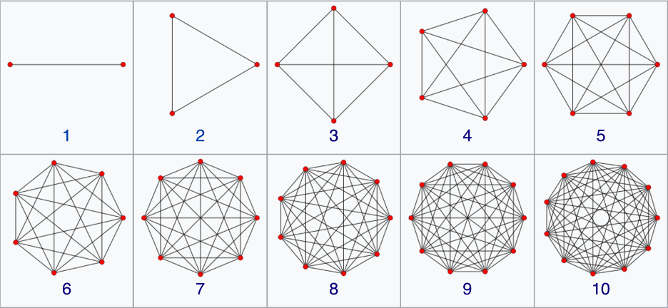
The N-simplex is the high-dimensional generalization of the tetrahedron.  It is a regular N-dimensional polytope with N+1 vertexes.  Starting at the bottom and going up, the simplexes are the point (0-simplex), the unit line (1-simplex), the equilateral triangle (2-simplex), the tetrahedron (3-simplex), the pentachoron (4-simplex), the hexateron (5-simplex) and onward.  When drawn on the two-dimensional plane, the simplexes are complete graphs with links connecting every node to every other node.  This dual character of equidistance and completeness give simplexes their utility. Each node is equivalent and is linked to each other.  There are N•(N-1)/2 links among N vertices, and there are (N-2)•(N-1)/2 triangular faces.

Fig. 1  The N-simplex structures from 1-D through 10-D.  Drawn on the 2D plane, the simplexes are complete graphs with links between every node.  The number of vertices is equal to the number of dimensions plus one. (Wikipedia)
Fig. 2 Coulomb-spring visualization of the energy minimization of a 12-simplex (a 12-dimensional tetrahedron). Each node is a charge. Each link is a spring. Beginning as a complete graph on the planar circle, it finds a minimum configuration with 3 internal nodes.

Construction of a d-simplex is recursive:  Begin with a (d-1)-dimensional simplex and add a point along an orthogonal dimension to construct a d-simplex.  For instance, to create a 2-simplex (an equilateral triangle), find the mid-point of the 1-simplex (a line segment)

            Centered 1-simplex:                (-1), (1)    

add a point on the perpendicular that is the same distance from each original vertex as the original vertices were distant from each other     

            Off-centered 2-simplex:         (-1,0), (1,0), (0, sqrt(3)/2)

Then shift the origin to the center of mass of the triangle

            Centered 2-simplex:               (-1, -sqrt(3)/6), (1, -sqrt(3)/6), (0, sqrt(3)/3)

The 2-simplex, i.e., the equilateral triangle, has a 1-simplex as each of its faces.  And each of those 1-simplexes has a 0-simplex as each of its ends.  Therefore, this recursive construction of ever higher-dimensional simplexes out of low-dimensional ones, provides an interesting pattern:

Fig. 3 The entries are the same numbers that appear in Pascal’s Triangle. (Wikipedia)

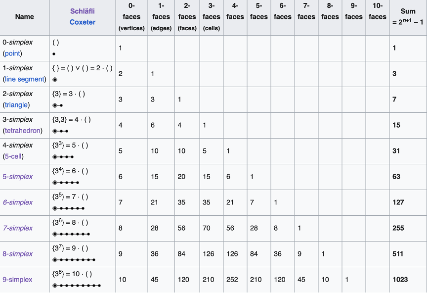
The coordinates of an N-simplex are not unique, although there are several convenient conventions.  One convention defines standard coordinates for an N-simplex in N+1 coordinate bases.  These coordinates embed the simplex into a space of one higher dimension.  For instance, the standard 2-simplex is defined by the coordinates (001), (010), (100) forming a two-dimensional triangle in three dimensions, and the simplex is a submanifold in the embedding space.  A more efficient coordinate choice matches the coordinate-space dimensionality to the dimensionality of the simplex.  Hence the 10 vertices of a 9-simplex can be defined by 9 coordinates (also not unique).  One choice is given in Fig. 4 for the 1-simplex up to the 9-simplex. 

Fig. 4 One possible set of coordinates for the 1-simplex up to the 9-simplex.  The center of mass of the simplex is at the origin, and the edge lengths are equal to 2.

The equations for the simplex coordinates are
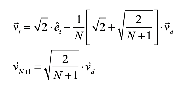
where

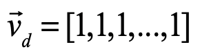
is the “diagonal” vector.  These coordinates are centered on the center of mass of the simplex, and the links all have length equal to 2 which can be rescaled by a multiplying factor.  The internal dihedral angle between all of the coordinate vectors for an N-simplex is

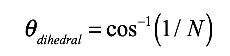
For moderate to high-dimensionality, the position vectors of the simplex vertices are pseudo-orthogonal.  For instance, for N = 9 the dihedral angle cosine is -1/9 = -0.111.  For higher dimensions, the simplex position vectors become asymptotically orthogonal.  Such orthogonality is an important feature for orthonormal decomposition of class superpositions, for instance of overlapping images.

Alloy Mixtures and Barycentric Coordinates

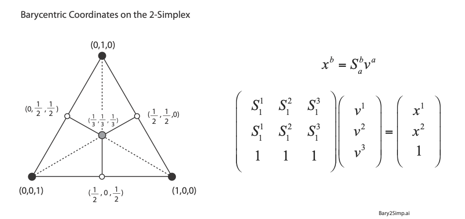
For linear systems, the orthonormality of basis representations is one of the most powerful features for system analysis in terms of superposition of normal modes.  Neural networks, on the other hand, are intrinsically nonlinear decision systems for which linear superposition does not hold inside the network, even if the symbols presented to the network are orthonormal superpositions.  This loss of orthonormality in deep networks can be partially retrieved by selecting the Simplex code.  It has pseudo-orthogonal probability distribution functions located on the vertices of the simplex.  There is an additional advantage to using the Simplex code: by using so-called barycentric coordinates, the simplex vertices can be expressed as independent bases.  An example for the 2-simplex is shown in Fig. 5.  The x-y Cartesian coordinates of the vertices (using tensor index notation) are given by (S11, S12), (S21, S22), and (S31, S32).  Any point (x1, x2) on the plane can be expressed as a linear combination of the three vertices with barycentric coordinates (v1, v2, v3) by solving for these three coefficients from the equation

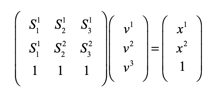
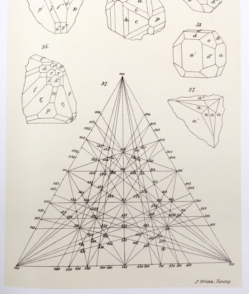
using Cramers rule.  For instance, the three vertices of the simplex are expressed using the 3-component barycentric coordinates (1,0,0), (0,1,0) and (0,0,1).  The mid-points on the edges have barycentric coordinates (1/2,1/2,0), (0,1/2,1/2), and (1/2,0,1/2).  The centroid of the simplex has barycentric coordinates (1/3,1/3,1/3).  Barycentric coordinates on a simplex are commonly used in phase diagrams of alloy systems in materials science. The simplex can also be used to identify crystallographic directions in three-dimensions, as in Fig. 6.

Fig. 5  Barycentric coordinates on the 2-Simplex.  The vertices represent “orthogonal” pure symbols.  Superpositions of 2 symbols lie on the edges.  Any point on the simplex can be represented using barycentric coordinates with three indices corresponding to the mixture of the three symbols.
Fig. 6 Crystallographic orientations expressed on a simplex. From A Treatise on Crystallography, William Miller, Cambridge (1839)

Replicator Dynamics on the Simplex

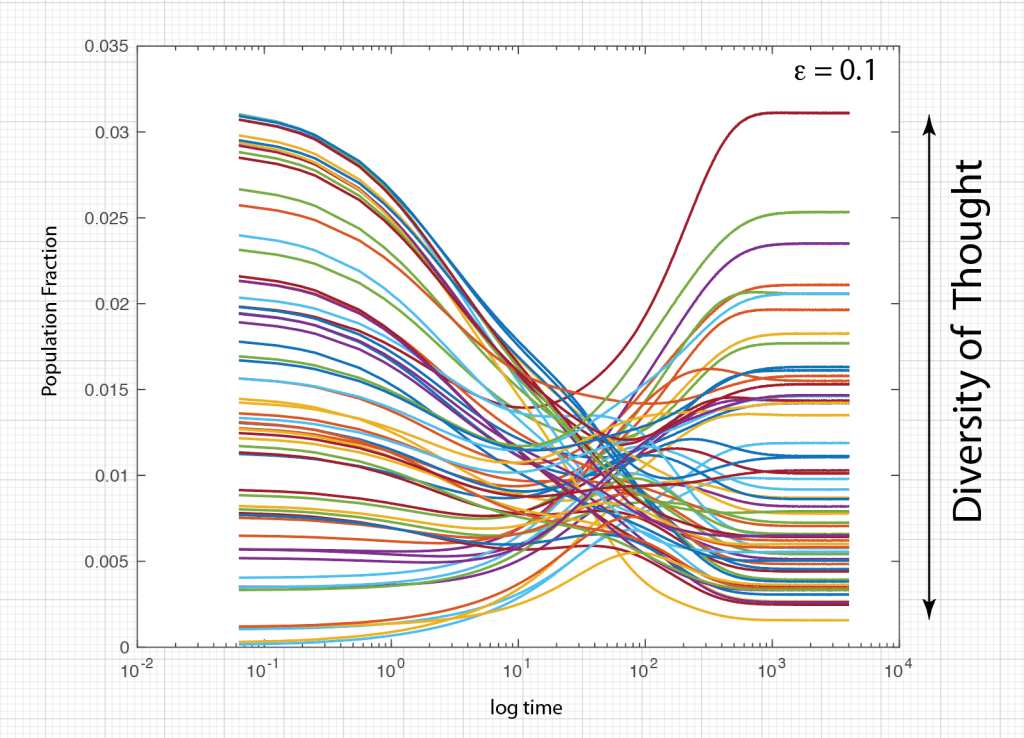
Ecosystems are among the most complex systems on Earth.  The complex interactions among hundreds or thousands of species may lead to steady homeostasis in some cases, to growth and collapse in other cases, and to oscillations or chaos in yet others.  But the definition of species can be broad and abstract, referring to businesses and markets in economic ecosystems, or to cliches and acquaintances in social ecosystems, among many other examples.  These systems are governed by the laws of evolutionary dynamics that include fitness and survival as well as adaptation. The dimensionality of the dynamical spaces for these systems extends to hundreds or thousands of dimensions—far too complex to visualize when thinking in four dimensions is already challenging. 

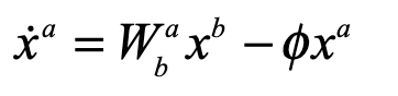
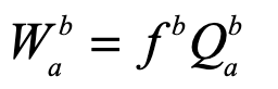
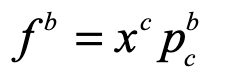
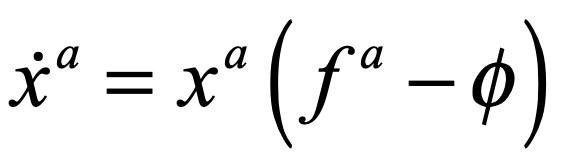
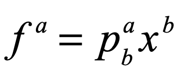
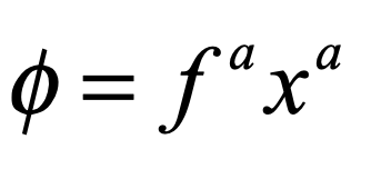
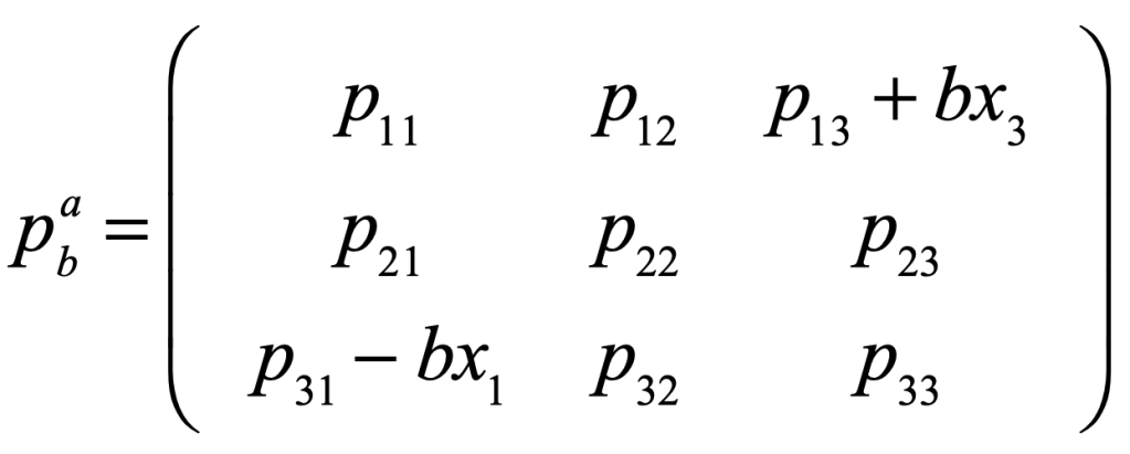
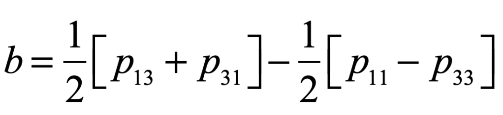
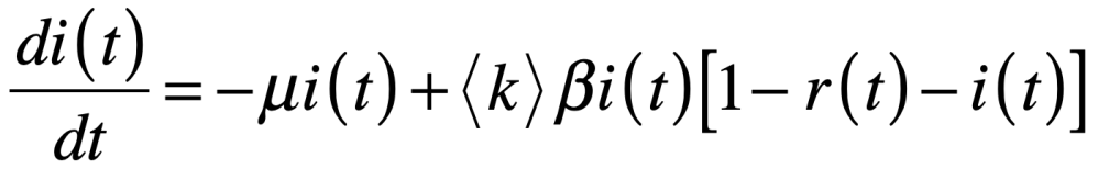
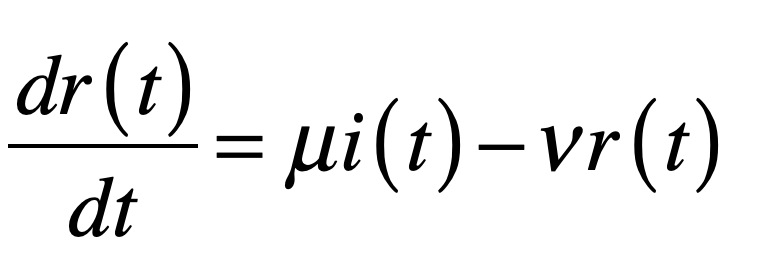
A classic model of interacting species is the replicator equation. It allows for a fitness-based proliferation and for trade-offs among the individual species. The replicator dynamics equations are shown in Fig. 7.

Fig. 7 Replicator dynamics has a surprisingly simple form, but with surprisingly complicated behavior. The key elements are the fitness and the payoff matrix. The fitness relates to how likely the species will survive. The payoff matrix describes how one species gains at the loss of another (although symbiotic relationships also occur).

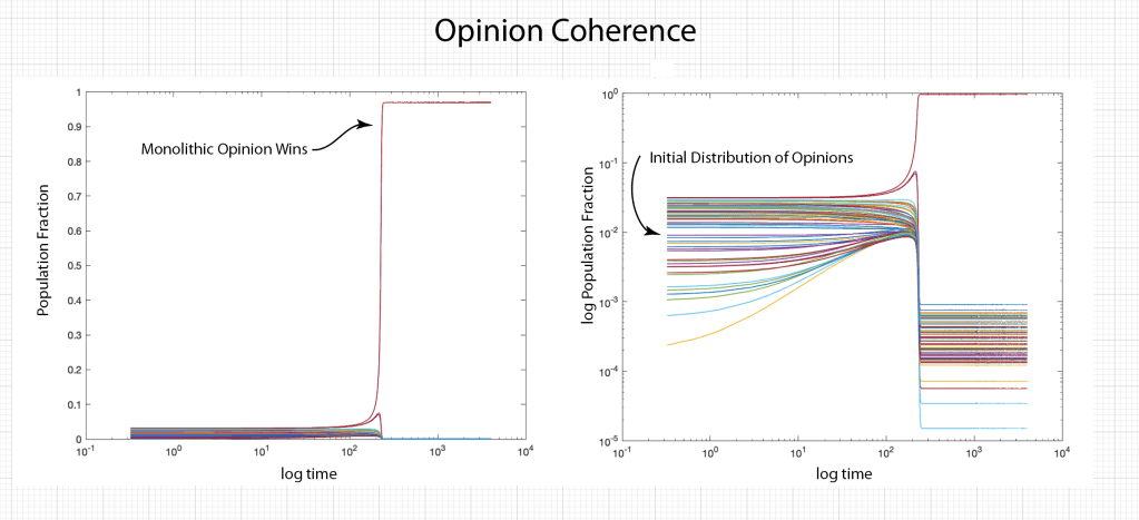
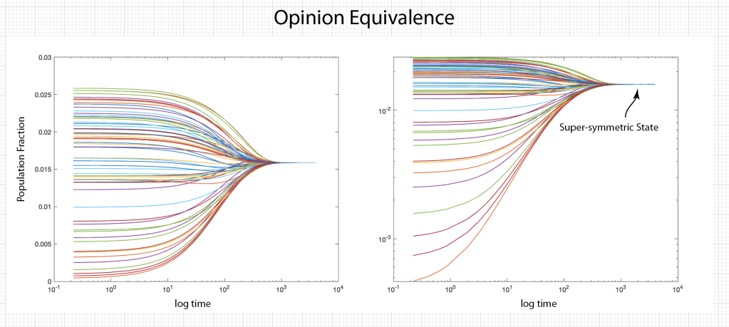
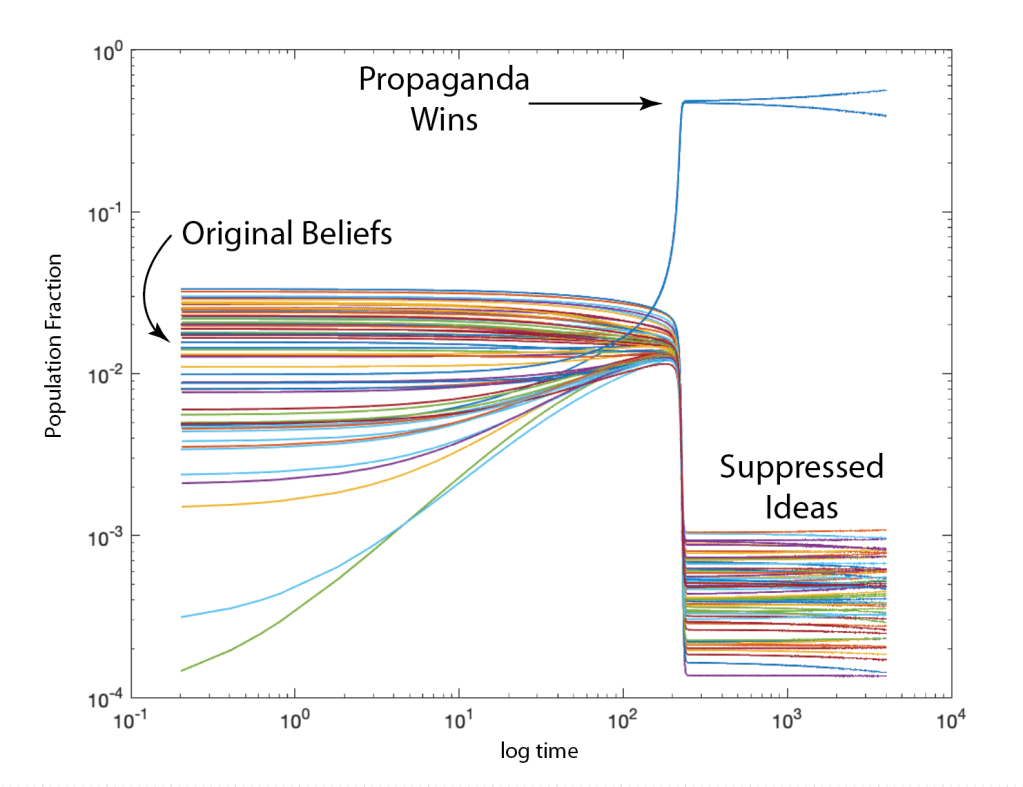
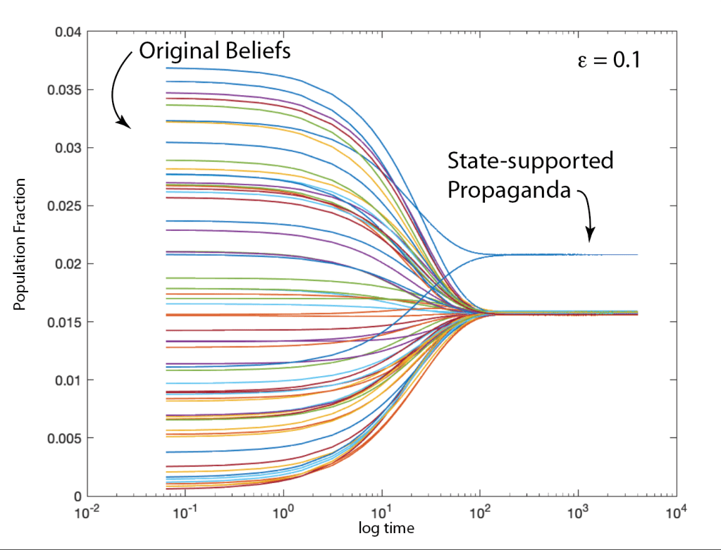
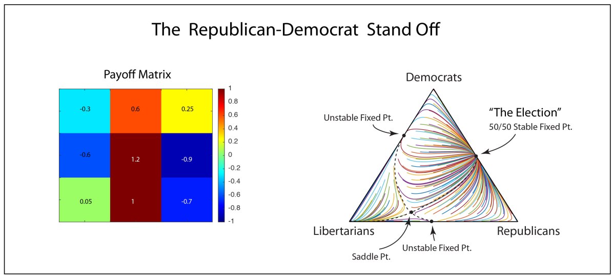
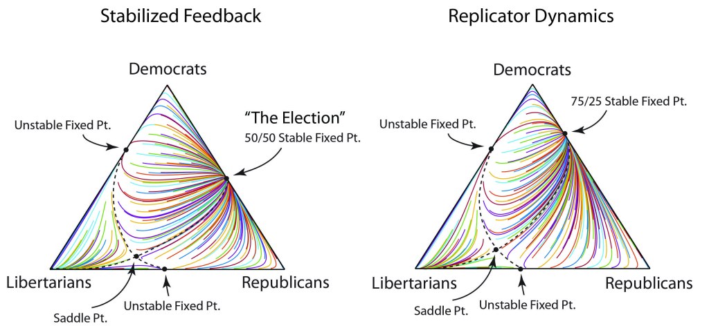
The population dynamics on the 2D simplex are shown in Fig. 8 for several different pay-off matrices (square matrix to the upper left of each simplex). The matrix values are shown in color and help interpret the trajectories. For instance the simplex on the upper-right shows a fixed point center. This reflects the antisymmetric character of the pay-off matrix around the diagonal. The stable spiral on the lower-left has a nearly asymmetric pay-off matrix, but with unequal off-diagonal magnitudes. The other two cases show central saddle points with stable fixed points on the boundary. A large variety of behaviors are possible for this very simple system. The Python program can be found in Trirep.py.

Fig. 8 Payoff matrix and population simplex for four random cases: Upper left is an unstable saddle. Upper right is a center. Lower left is a stable spiral. Lower right is a marginal case.

Linear Programming with the Dantzig Simplex

There is a large set of optimization problems in which a linear objective function is to be minimized subject to a set of inequalities. This is known as “Linear Programming”. These LP systems can be expressed as

The vector index goes from 1 to d, the dimension of the space. Each inequality creates a hyperplane, where two such hyperplanes intersect along a line terminated at each end by a vertex point. The set of vertexes defines a polytope in d-dimensions, and each face of the polytope, when combined with the point at the origin, defines a 3-simplex.

It is easy to visualize in lower dimensions why the linear objective function must have an absolute minimum at one of the vertexes of the polytope. And finding that minimum is a trivial exercise: Start at any vertex. Poll each neighboring vertex and move to the one that has the lowest value of the objective function. Repeat until the current vertex has a lower objective value than any neighbors. Because of the linearity of the objective function, this is a unique minimum (except for rare cases of accidental degeneracy). This iterative algorithm defines a walk on the vertexes of the polytope.

The question arises, why not just evaluate the objection function at each vertex and then just pick the vertex with the lowest value? The answer in high dimensions is that there are too many vertexes, and finding all of them is inefficient. If there are N vertexes, the walk to the solution visits only a few of the vertexes, on the order of log(N). The algorithm therefore scales as log(N), just like a search tree.

Fig. 9 Dantzig simplex approach on a convex 3D space of basic solutions in a linear programming problem.

This simple algorithm was devised by George Dantzig (1914 – 2005) in 1939 when he was a graduate student at UC Berkeley. He had arrived late to class and saw two problems written on the chalk board. He assumed that these were homework assignments, so he wrote them down and worked on them over the following week. He recalled that they seemed a bit harder than usual, but he eventually solved them and turned them in. A few weeks later, his very excited professor approached him and told him that the problems weren’t homework–they were two of the most important outstanding problems in optimization and that Dantzig had just solved them! The 1997 movie Good Will Hunting, with Matt Damon, Ben Affleck, and Robin Williams, borrowed this story for the opening scene.

The Amoeba Simplex Crawling through Hyperspace

Unlike linear programming problems with linear objective functions, multidimensional minimization of nonlinear objective functions is an art unto itself, with many approach. One of these is a visually compelling algorithm that does the trick more often than not. This is the so-called amoeba algorithm that shares much in common with the Dantzig simplex approach to linear programming, but instead of a set of fixed simplex coordinates, it uses a constantly shifting d-dimensional simplex that “crawls” over the objective function, seeking its minimum.

One of the best descriptions of the amoeba simplex algorithm is in “Numerical Recipes” [4] that describes the crawling simplex as

When it reaches a “valley floor”, the method contracts itself in the transverse direction and tries to ooze down the valley. If there is a situation where the simplex is trying to “pass through the eye of a needle”, it contracts itself in all directions, pulling itself in around its lowest (best) point.

(From Press, Numerical Recipes, Cambridge)

The basic operations for the crawling simplex are reflection and scaling. For a given evaluation of all the vertexes of the simplex, one will have the highest value and another the lowest. In a reflection, the highest point is reflected through the d-dimensional face defined by the other d vertexes. After reflection, if the new evaluation is lower than the former lowest value, then the point is expanded. If, on the other hand, it is little better than it was before reflection, then the point is contracted. The expansion and contraction are what allows the algorithm to slide through valleys or shrink to pass through the eye of a needle.

The amoeba algorithm was developed by John Nelder and Roger Mead in 1965 at a time when computing power was very limited. The algorithm works great as a first pass at a minimization problem, and it almost always works for moderately small dimensions, but for very high dimensions there are more powerful algorithms today for optimization, built into all the deep learning software environments like Tensor Flow and the Matlab toolbox.


[1] M. Hillert, Phase equilibria, phase diagrams and phase transformations : their thermodynamic basis.  (Cambridge University Press, Cambridge, UK ;, ed. 2nd ed., 2008).

[2] P. Schuster, K. Sigmund, Replicator Dynamics. Journal of Theoretical Biology 100, 533-538 (1983); P. Godfrey-Smith, The replicator in retrospect. Biology & Philosophy 15, 403-423 (2000).

[3] R. E. Stone, C. A. Tovey, The Simplex and Projective Scaling Algorithms as Iteratively Reweighted Least-squares Methods. Siam Review 33, 220-237 (1991).

[4] W. H. Press, Numerical Recipes in C++ : The Art of Scientific Computing.  (Cambridge University Press, Cambridge, UK; 2nd ed., 2002).

Democracy against Authoritarians: The Physics of Public Opinion

An old joke goes that Democracy is a terrible form of government … except it’s better than all the others!

Our world today is faced with conflict between democracy and dictatorship. On the one side is the free world, where leaders are chosen by some form of representation of large numbers of citizens and sometimes even a majority. On the other side is authoritarianism where a select few are selected by a select few to govern everyone else.

[I]t has been said that democracy is the worst form of Government except all those other forms that have been tried from time to time; but there is the broad feeling in our country that the people should rule, and that public opinion expressed by all constitutional means, should shape, guide, and control the actions of Ministers who are their servants and not their masters.

Winston Churchill (1947)

An argument in favor of democracy is freedom of choice for the largest segment of the population, plus the ability to remove leaders who fail to provide for the perceived welfare of the most citizens. This makes democracy adaptive, shifting with the times. It also makes leaders accountable for their actions and crimes. An argument in favor of authoritarianism is the myth of the benevolent dictator–someone who knows what’s best for the people even if the people don’t know it themselves.

But dictators are rarely benevolent, and as they become saturated with power, they are corrupted. The criminal massacres, perpetrated by Putin, of Ukrainian civilians is one of the strongest recent arguments against authoritarianism. A single man decides, on a whim, the life and death of thousands or maybe more. The invasion of Ukraine is so egregious and unwarranted, that we wonder how the Russian people can put up with their isolated and manic leader. Yet by some measure more than 60% of the people in Russia approve of the war.

How can the free world see the invasion as the atrocity it is, while Russia’s majority sees it as a just war? The answer is a surprising result of population dynamics known as the replicator-mutator equation. The challenge for us here in the free world is to learn how to game the replicator-mutator equation to break up the monopoly of popular opinion and make Putin pay for his arrogance. This blog explains how “mass hysteria” can arise from forces within a complex environment, and how to construct a possible antidote.

Replicator-Mutator Equation

There are several simple models of population dynamics that try to explain the rise and fall of the number of individuals that belong to varying cohorts within the population. These models incorporate aspects of relative benefit of one group over another, plus the chance to change sides–defection. The dynamics under these conditions can be highly nonlinear and highly non-intuitive. One of the simplest of these models is known as the replicator-mutator model where replication follows the fitness of the cohort, and where individuals can defect to a “more fit” cohort.

The basic dynamics of the model are

where xa is the fraction of the population that is in cohort a, Wab is a transition probability, and φ is the average fitness of the full population. The transition matrix is given by

where fb is the fitness of cohort b and Qba is a stochastic matrix that allows for defection of an individual from one cohort to another. The fitness of a cohort is given by

where pbc is the pay-off matrix for the relative benefit of one cohort at the expense of another. Finally the average fitness is

The Einstein implicit summation convention is assumed in all of these equations, and the metric space in which the dynamics are embedded is “flat” so that there is no essential difference between superscripts and subscripts. There is also a conservation law that the sum over all population fractions equals unity.

In the language of population dynamics, this model has frequency-dependent fitness, with defection and pay-off, in a zero-sum game.

One of the simplest questions to answer with this model is how so many people can come to believe one thing. This is known as “opinion uniformity”.

Uniformity versus Diversity

This replicator-mutator model explains the property of opinion uniformity, as well as the opposite extreme of opinion diversity. The starting point for both is the pay-off matrix pbc which is assumed to be unity on the diagonal for b = c and to a constant factor a for b ~= c. This pay-off is symmetric so that all opinions are equally “believable”. The stochastic defection matrix is close to unity on the diagonal, and has random terms on the off-diagonal that are proportional to a constant ε. The defection matrix allows a person from one cohort to defect to the belief system of another cohort if they believe that the new cohort has more merit. Cohorts with greater merit (fitness) gain more members over time, while cohorts with lower merit have fewer members over time.

Note that the fitness increases with the number of members in the cohort. This is the bandwagon effect. A belief system is perceived to have more merit if there are more people who believe it. This clearly creates a positive feedback that would cause this cohort to grow. Even though all the cohorts have this same positive feedback, the zero-sum rule only allows one of the cohorts to grow to its maximum extent, taking members away from all the other cohorts. This is illustrated in Fig. 1. One belief system wins, taking almost the full population with it.

Fig. 1 Population fractions evolving as a function of time for a = 0.5 and a small defection rate ε = 0.02. One winner takes almost all the population. These are two views of the same data on semilog and log-log.

What allows the winner to take all is the positive feedback where the fitness of the cohort increases with the number of members, combined with the ability for that cohort to take members from other cohorts through the defection matrix.

However, all of the cohorts are trying the same thing, and the pay-off matrix is fully symmetric and equal for all cohorts, so no cohort is intrinsically “better” than another. This property opens the door to a strong alternative to opinion uniformity. In fact, as more members are allowed to defect, it creates a trend counter to winner-take-all, helping to equalize the cohorts. Suddenly, a bifurcation is passed when the winner-take-all converts discontinuously to a super-symmetric situation when all opinions are held by equal numbers of people. This is illustrated in Fig. 2 for a slightly higher defection rate ε = 0.03. The parameters are identical to those in Fig. 1, but the higher defection rate stabilizes the super-symmetric state of maximum diversity.

Fig. 2 Population fractions for higher defection rate of 0.03. In super-symmetric state, all opinions are held at the same rate with maximum diversity.

These two extreme results of the replicator-mutator equation, that switch suddenly from one to the other dependent on the defection rate, may seem to produce solutions neither of which are ideal for a healthy democracy. One the one hand, in the uniform case where the wining opinion is monolithic, everyone is a carbon-copy of everyone else, which is a form of cultural death (lack of diversity). But, on the other hand, one might argue that maximum opinion diversity is just as concerning, because no-one can agree on anything. If all opinions are equivalent, then everyone in the society believes something different and there is no common ground. But in the diversity case, at least there is no state-level control of the population. In the case of opinion uniformity, the wining opinion can be manipulated by propaganda.

The Propaganda Machine

A government can “seed” the belief networks with propaganda that favors the fitness of what they want their citizens to hear. Because of the positive feedback, any slight advantage of one opinion over others can allow that opinion to gain large numbers through the bandwagon effect. Of course, even stronger control that stifles dissent, for instance by shutting down the free press, makes it that much more likely that the state-controlled story is believed. This may be one reason for the 60% (as of the writing of this blog) support Putin’s war, despite the obvious lies that are being told. This is illustrated in Fig. 3 by boosting the payoff between two similar lies that the government wants its people to believe. These rise to take about 60% of the population. Members of the cohort are brain-washed, not by the government alone, but by all their neighbors who are parroting the same thing.

Fig. 3 Government propaganda acts as a “seed” that makes the propaganda grow faster than other beliefs, even for a defection rate of 0.03 which is above the threshold of Fig. 2.

Breaking the Monopoly of Thought

How do we fight back? Not just against the Kremlin’s propaganda, but also against QANON and Trump’s Big Lie and the pernicious fallacy of nationalism? The answer is simple: diversity of thought! The sliver bullet in the replicator-mutator model is the defection matrix. The existence of a bifurcation means that a relatively small increase in the amount of diverse opinion, and the freedom to swap opinions, can lead to a major qualitative collapse of the monolithic thought, even when supported by government propaganda, as shown in Fig. 4. More people may still believe in the state-supported propaganda than the others, but it is no longer a majority.

Fig. 4 Increasing the defection rate can help equalize free opinions against the state-supported propaganda

The above models were all very homogeneous. It is more realistic that people are connected through small-world networks. In this case, there is much more diversity, as shown in Fig. 5, although the defection rate needs to be much higher to prevent a monolithic opinion from dominating. The state-supported propaganda is buried in the resulting mix of diverse ideas. Therefore, to counteract state control, people must feel free to hop about in their choice of beliefs and have access to other beliefs.

Fig. 5 The defection matrix is multiplied by the adjacency matrix of a small-world network. There is significant diversity of thought, but a relatively high defection rate is needed. The state-supported propaganda is buried in this mix.

This is a bit paradoxical. On the one hand, the connectivity of the internet has fostered the rise of conspiracy theories and other odd-ball ideas. But sustained access to multiple sources of information is the best defense against all that crazy stuff winning out. In other words, not only do we have to put up with the lunatic fringe if we are to have full diversity of thought, but we need to encourage everyone to feel free to “shop around” for different ideas, even if some of them are crazy. Our free society shouldn’t be cancelling people who have divergent opinions, because that sets us down the path to authoritarianism. As a recent add said in the New York Times, “Cancel culture cancels culture.” Unfortunately, authoritarianism is on the rise around the world, and the US almost suffered that fate on Jan. 6, 2021. Furthermore, with Xi aligning with Putin and giving him the green light on Ukraine–cynically on the eve of the Olympic Games (of peace)–the new world order will revolve around that axis for decades to come, if the world survives that long. Diversity and freedom may be the only antidote.

By David D. Nolte, March 24, 2022

Matlab Program: Repmut.m

function repmut
% https://github.itap.purdue.edu/nolte/Matlab-Programs-for-Nonlinear-Dynamics

clear
format compact

N = 63;     
p = 0.5;

mutype = 1;     % 0 = Hamming   1 = rand
pay = 1;        % 0 = Hamming   1 = 1/sqrt(N) 
ep = 0.5;      % average mutation rate: 0.1 to 0.01 typical  (0.4835)

%%%%% Set original population
x0temp = rand(1,N);    % Initial population
sx = sum(x0temp);
y0 = x0temp/sx;
Pop0 = sum(y0);


%%%%% Set Adjacency

%node = makeglobal(N);
%node = makeER(N,0.25);       % 0.5     0.25 
%node = makeSF(N,6);       % 12         6
node = makeSW(N,7,0.125);   % 15,0.5    7,0.5
[Adj,degree,Lap] = adjacency(node);

%%%%%% Set Hamming distance
for yloop = 1:N
    for xloop = 1:N
        H(yloop,xloop) = hamming(yloop-1,xloop-1);
    end
end

%%%%%%% Set Mutation matrix
if mutype == 0
    Qtemp = 1./(1+H/ep);    %Mutation matrix on Hamming
    Qsum = sum(Qtemp,2);
    mnQsum = mean(Qsum);
    
    % Normalize mutation among species
    for yloop = 1:N
        for xloop = 1:N
            Q(yloop,xloop) = Qtemp(yloop,xloop)/Qsum(xloop);
        end
    end
    
elseif mutype == 1  
    S = stochasticmatrix(N);
    Stemp = S - diag(diag(S));
    Qtemp = ep*Stemp;
    sm = sum(Qtemp,2)';
    Q = Qtemp + diag(ones(1,N) - sm);
end

figure(1)
imagesc(Q)
title('Mutation Matrix')
colormap(jet)

%%%%%%% Set payoff matrix
if pay == 1
    payoff = zeros(N,N);
    for yloop = 1:N
        payoff(yloop,yloop) = 1;
        for xloop = yloop + 1:N
            payoff(yloop,xloop) = p;
            payoff(xloop,yloop) = p;
            payoff(1,N) = 1;    % Propaganda
            payoff(N,1) = 1;
        end
    end
elseif pay == 0
    payoff = zerodiag(exp(-1*H));
end

figure(2)
imagesc(payoff)
title('Payoff Matrix')
colormap(jet)

% Run time evolution
tspan = [0 4000];
[t,x] = ode45(@quasispec,tspan,y0);

Pop0
[sz,dum] = size(t);
Popend = sum(x(sz,:))

for loop = 1:N
    fit(loop) = sum(payoff(:,loop)'.*x(sz,:));
end

phistar = sum(fit.*x(sz,:))       % final average fitness

xend = x(sz,:)
sortxend = sort(xend,'descend');
coher = sum(sortxend(1:2))

figure(3)
clf
h = colormap(lines);
for loop = 1:N
    plot(t,x(:,loop),'Color',h(round(loop*64/N),:),'LineWidth',1.25)
    hold on
end
hold off

figure(4)
clf
for loop = 1:N
    semilogx(t,x(:,loop),'Color',h(round(loop*64/N),:),'LineWidth',1.25)
    hold on
end
hold off

figure(5)
clf
for loop = 1:N
    semilogy(t,x(:,loop),'Color',h(round(loop*64/N),:),'LineWidth',1.25)
    hold on
end
hold off

figure(6)
clf
for loop = 1:N
    loglog(t,x(:,loop),'Color',h(round(loop*64/N),:),'LineWidth',1.25)
    hold on
end
hold off

%%%%%%%%%%%%%%%%%%%%%%%%%%%%%%%%%%%%%%
%
%
%%%%%%%%%%%%%%%%%%%%%%%%%%%%%%%%%%%%%%
    function yd = quasispec(~,y)
        
        for floop = 1:N
            f(floop) = sum(payoff(:,floop).*y);
        end
        
        Connect = Adj + eye(N);
        
        % Transition matrix
        for yyloop = 1:N
            for xxloop = 1:N
                W(yyloop,xxloop) = f(yyloop)*(Connect(yyloop,xxloop)*Q(yyloop,xxloop));
            end
        end
        
        phi = sum(f'.*y);   % Average fitness of population
        
        yd = W*y - phi*y;
        
    end     % end quasispec
end

Further Reading

M. A. Nowak, Evolutionary Dynamics: Exploring the Equations of Life. Cambridge, Mass.: Harvard University Press, 2006.

The Physics of U. S. Presidential Elections (why are so many elections so close?)

Well here is another squeaker! The 2020 U. S. presidential election was a dead heat. What is most striking is that half of the past six US presidential elections have been won by less than 1% of the votes cast in certain key battleground states. For instance, in 2000 the election was won in Florida by less than 1/100th of a percent of the total votes cast.

How can so many elections be so close? This question is especially intriguing when one considers the 2020 election, which should have been strongly asymmetric, because one of the two candidates had such serious character flaws. It is also surprising because the country is NOT split 50/50 between urban and rural populations (it’s more like 60/40). And the split of Democrat/Republican is about 33/29 — close, but not as close as the election. So how can the vote be so close so often? Is this a coincidence? Or something fundamental about our political system? The answer lies (partially) in nonlinear dynamics coupled with the libertarian tendencies of American voters.

Rabbits and Sheep

Elections are complex dynamical systems consisting of approximately 140 million degrees of freedom (the voters). Yet US elections are also surprisingly simple. They are dynamical systems with only 2 large political parties, and typically a very small third party.

Voters in a political party are not too different from species in an ecosystem. There are many population dynamics models of things like rabbit and sheep that seek to understand the steady-state solutions when two species vie for the same feedstock (or two parties vie for the same votes). Depending on reproduction rates and competition payoff, one species can often drive the other species to extinction. Yet with fairly small modifications of the model parameters, it is often possible to find a steady-state solution in which both species live in harmony. This is a symbiotic solution to the population dynamics, perhaps because the rabbits help fertilize the grass for the sheep to eat, and the sheep keep away predators for the rabbits.

There are two interesting features to such a symbiotic population-dynamics model. First, because there is a stable steady-state solution, if there is a perturbation of the populations, for instance if the rabbits are culled by the farmer, then the two populations will slowly relax back to the original steady-state solution. For this reason, this solution is called a “stable fixed point”. Deviations away from the steady-state values experience an effective “restoring force” that moves the population values back to the fixed point. The second feature of these models is that the steady state values depend on the parameters of the model. Small changes in the model parameters then cause small changes in the steady-state values. In this sense, this stable fixed point is not fundamental–it depends on the parameters of the model.

Fig. 1 Dynamics of rabbits and sheep competing for the same resource (grass). For these parameters, one species dies off while the other thrives. A slight shift in parameters can turn the central saddle point into a stable fixed point where sheep and rabbits coexist in stead state. ([1] Reprinted from Introduction to Modern Dynamics (Oxford University Press, 2019) pg. 119)

But there are dynamical models which do have a stability that maintains steady values even as the model parameters shift. These models have negative feedback, like many dynamical systems, but if the negative feedback is connected to winner-take-all outcomes of game theory, then a robustly stable fixed point can emerge at precisely the threshold where such a winner would take all.

The Replicator Equation

The replicator equation provides a simple model for competing populations [2]. Despite its simplicity, it can model surprisingly complex behavior. The central equation is a simple growth model

where the growth rate depends on the fitness fa of the a-th species relative to the average fitness φ of all the species. The fitness is given by

where pab is the payoff matrix among the different species (implicit Einstein summation applies). The fitness is frequency dependent through the dependence on xb. The average fitness is

This model has a zero-sum rule that keeps the total population constant. Therefore, a three-species dynamics can be represented on a two-dimensional “simplex” where the three vertices are the pure populations for each of the species. The replicator equation can be applied easily to a three-party system, one simply defines a payoff matrix that is used to define the fitness of a party relative to the others.

The Nonlinear Dynamics of Presidential Elections

Here we will consider the replicator equation with three political parties (Democratic, Republican and Libertarian). Even though the third party is never a serious contender, the extra degree of freedom provided by the third party helps to stabilize the dynamics between the Democrats and the Republicans.

It is already clear that an essentially symbiotic relationship is at play between Democrats and Republicans, because the elections are roughly 50/50. If this were not the case, then a winner-take-all dynamic would drive virtually everyone to one party or the other. Therefore, having 100% Democrats is actually unstable, as is 100% Republicans. When the populations get too far out of balance, they get too monolithic and too inflexible, then defections of members will occur to the other parties to rebalance the system. But this is just a general trend, not something that can explain the nearly perfect 50/50 vote of the 2020 election.

To create the ultra-stable fixed point at 50/50 requires an additional contribution to the replicator equation. This contribution must create a type of toggle switch that depends on the winner-take-all outcome of the election. If a Democrat wins 51% of the vote, they get 100% of the Oval Office. This extreme outcome then causes a back action on the electorate who is always afraid when one party gets too much power.

Therefore, there must be a shift in the payoff matrix when too many votes are going one way or the other. Because the winner-take-all threshold is at exactly 50% of the vote, this becomes an equilibrium point imposed by the payoff matrix. Deviations in the numbers of voters away from 50% causes a negative feedback that drives the steady-state populations back to 50/50. This means that the payoff matrix becomes a function of the number of voters of one party or the other. In the parlance of nonlinear dynamics, the payoff matrix becomes frequency dependent. This goes one step beyond the original replicator equation where it was the population fitness that was frequency dependent, but not the payoff matrix. Now the payoff matrix also becomes frequency dependent.

The frequency-dependent payoff matrix (in an extremely simple model of the election dynamics) takes on negative feedback between two of the species (here the Democrats and the Republicans). If these are the first and third species, then the payoff matrix becomes

where the feedback coefficient is

and where the population dependences on the off-diagonal terms guarantee that, as soon as one party gains an advantage, there is defection of voters to the other party. This establishes a 50/50 balance that is maintained even when the underlying parameters would predict a strongly asymmetric election.

For instance, look at the dynamics in Fig. 2. For this choice of parameters, the replicator model predicts a 75/25 win for the democrats. However, when the feedback is active, it forces the 50/50 outcome, despite the underlying advantage for the original parameters.

Fig. 2 Comparison of the stabilized election with 50/50 outcome compared to the replicator dynamics without the feedback. For the parameters chosen here, there would be a 75/25 victory of the Democrats over the Republications. However, when the feedback is in play, the votes balance out at 50/50.

There are several interesting features in this model. It may seem that the Libertarians are irrelevant because they never have many voters. But their presence plays a surprisingly important role. The Libertarians tend to stabilize the dynamics so that neither the democrats nor the republicans would get all the votes. Also, there is a saddle point not too far from the pure Libertarian vertex. That Libertarian vertex is an attractor in this model, so under some extreme conditions, this could become a one-party system…maybe not Libertarian in that case, but possibly something more nefarious, of which history can provide many sad examples. It’s a word of caution.

Disclaimers and Caveats

No attempt has been made to actually mode the US electorate. The parameters in the modified replicator equations are chosen purely for illustration purposes. This model illustrates a concept — that feedback in the payoff matrix can create an ultra-stable fixed point that is insensitive to changes in the underlying parameters of the model. This can possibly explain why so many of the US presidential elections are so tight.

Someone interested in doing actual modeling of US elections would need to modify the parameters to match known behavior of the voting registrations and voting records. The model presented here assumes a balanced negative feedback that ensures a 50/50 fixed point. This model is based on the aversion of voters to too much power in one party–an echo of the libertarian tradition in the country. A more sophisticated model would yield the fixed point as a consequence of the dynamics, rather than being a feature assumed in the model. In addition, nonlinearity could be added that would drive the vote off of the 50/50 point when the underlying parameters shift strongly enough. For instance, the 2008 election was not a close one, in part because the strong positive character of one of the candidates galvanized a large fraction of the electorate, driving the dynamics away from the 50/50 balance.

References

[1] D. D. Nolte, Introduction to Modern Dynamics: Chaos, Networks, Space and Time (Oxford University Press, 2019) 2nd Edition.

[2] Nowak, M. A. (2006). Evolutionary Dynamics: Exploring the Equations of Life. Cambridge, Mass., Harvard University Press.

Physics in the Age of Contagion: Part 4. Fifty Shades of Immunity to COVID-19

This is the fourth installment in a series of blogs on the population dynamics of COVID-19. In my first blog I looked at a bifurcation physics model that held the possibility (and hope) that with sufficient preventive action the pandemic could have died out and spared millions. That hope was in vain.

What will it be like to live with COVID-19 as a constant factor of modern life for years to come?

In my second blog I looked at a two-component population dynamics model that showed the importance of locking down and not emerging too soon. It predicted that waiting only a few extra weeks before opening could have saved tens of thousands of lives. Unfortunately, because states like Texas and Florida opened too soon and refused to mandate the wearing of masks, thousands of lives were lost.

In my third blog I looked at a network physics model that showed the importance of rapid testing and contact tracing to remove infected individuals to push the infection rate low — not only to flatten the curve, but to drive it down. While most of the developed world is succeeding in achieving this, the United States is not.

In this fourth blog, I am looking at a simple mean-field model that shows what it will be like to live with COVID-19 as a constant factor of modern life for years to come. This is what will happen if the period of immunity to the disease is short and people who recover from the disease can get it again. Then the disease will never go away and the world will need to learn to deal with it. How different that world will look from the one we had just a year ago will depend on the degree of immunity that is acquired after infection, how long a vaccine will provide protection before booster shots are needed, and how many people will get the vaccine or will refus.

SIRS for SARS

COVID-19 is a SARS corona virus known as SARS-CoV-2. SARS stands for Severe Acute Respiratory Syndrome. There is a simple and well-established mean-field model for an infectious disease like SARS that infects individuals, from which they recover, but after some lag period they become susceptible again. This is called the SIRS model, standing for Susceptible-Infected-Recovered-Susceptible. This model is similar to the SIS model of my first blog, but it now includes a mean lifetime for the acquired immunity, after an individual recovers from the infection and then becomes susceptible again. The bifurcation threshold is the same for the SIRS model as the SIS model, but with SIRS there is a constant susceptible population. The mathematical flow equations for this model are

where i is the infected fraction, r is the recovered fraction, and 1 – i – r = s is the susceptible fraction. The infection rate for an individual who has k contacts is βk. The recovery rate is μ and the mean lifetime of acquired immunity after recovery is τlife = 1/ν. This model assumes that all individuals are equivalent (no predispositions) and there is no vaccine–only natural immunity that fades in time after recovery.

The population trajectories for this model are shown in Fig. 1. The figure on the left is a 3-simplex where every point in the triangle stands for a 3-tuple (i, r, s). Our own trajectory starts at the right bottom vertex and generates the green trajectory that spirals into the fixed point. The parameters are chosen to be roughly equivalent to what is known about the virus (but with big uncertainties in the model parameters). One of the key results is that the infection will oscillate over several years, settling into a steady state after about 4 years. Thereafter, there is a steady 3% infected population with 67% of the population susceptible and 30% recovered. The decay time for the immunity is assumed to be one year in this model. Note that the first peak in the infected numbers will be about 1 year, or around March 2021. There is a second smaller peak (the graph on the right is on a vertical log scale) at about 4 years, or sometime in 2024.

Fig. 1 SIRS model for COVID-19 in which immunity acquired after recovery fades in time so an individual can be infected again. If immunity fades and there is never a vaccine, a person will have an 80% chance of getting the virus at least twice in their lifetime, and COVID will become the third highest cause of death in the US after heart disease and cancer.

Although the recovered fraction is around 30% for these parameters, it is important to understand that this is a dynamic equilibrium. If there is no vaccine, then any individual who was once infected can be infected again after about a year. So if they don’t get the disease in the first year, they still have about a 4% chance to get it every following year. In 50 years, a 20-year-old today would have almost a 90% chance of having been infected at least once and an 80% chance of having gotten it at least twice. In other words, if there is never a vaccine, and if immunity fades after each recovery, then almost everyone will eventually get the disease several times in their lifetime. Furthermore, COVID will become the third most likely cause of death in the US after heart disease (first) and cancer (second). The sad part of this story is that it all could have been avoided if the government leaders of several key nations, along with their populations, had behaved responsibly.

The Asymmetry of Personal Cost under COVID

The nightly news in the US during the summer of 2020 shows endless videos of large parties, dense with people, mostly young, wearing no masks. This is actually understandable even though regrettable. It is because of the asymmetry of personal cost. Here is what that means …

On any given day, an individual who goes out and about in the US has only about a 0.01 percent chance of contracting the virus. In the entire year, there is only about a 3% chance that that individual will get the disease. And even if they get the virus, they only have a 2% chance of dying. So the actual danger per day per person is so minuscule that it is hard to understand why it is so necessary to wear a mask and socially distance. Therefore, if you go out and don’t wear a mask, almost nothing bad will happen to YOU. So why not? Why not screw the masks and just go out!

And this is why that’s such a bad idea: because if no-one wears a mask, then tens or hundreds of thousands of OTHERS will die.

This is the asymmetry of personal cost. By ignoring distancing, nothing is likely to happen to YOU, but thousands of OTHERS will die. How much of your own comfort are you willing to give up to save others? That is the existential question.

This year is the 75th anniversary of the end of WW II. During the war everyone rationed and recycled, not because they needed it for themselves, but because it was needed for the war effort. Almost no one hesitated back then. It was the right thing to do even though it cost personal comfort. There was a sense of community spirit and doing what was good for the country. Where is that spirit today? The COVID-19 pandemic is a war just as deadly as any war since WW II. There is a community need to battle it. All anyone has to do is wear a mask and behave responsibly. Is this such a high personal cost?

The Vaccine

All of this can change if a reliable vaccine can be developed. There is no guarantee that this can be done. For instance, there has never been a reliable vaccine for the common cold. A more sobering thought is to realize is that there has never been a vaccine for the closely related virus SARS-CoV-1 that broke out in 2003 in China but was less infectious. But the need is greater now, so there is reason for optimism that a vaccine can be developed that elicits the production of antibodies with a mean lifetime at least as long as for naturally-acquired immunity.

The SIRS model has the same bifurcation threshold as the SIS model that was discussed in a previous blog. If the infection rate can be made slower than the recovery rate, then the pandemic can be eliminated entirely. The threshold is

The parameter μ, the recovery rate, is intrinsic and cannot be changed. The parameter β, the infection rate per contact, can be reduced by personal hygiene and wearing masks. The parameter <k>, the average number of contacts to a susceptible person, can be significantly reduced by vaccinating a large fraction of the population.

To simulate the effect of vaccination, the average <k> per person can be reduced at the time of vaccination. This lowers the average infection rate. The results are shown in Fig. 2 for the original dynamics, a vaccination of 20% of the populace, and a vaccination of 40% of the populace. For 20% vaccination, the epidemic is still above threshold, although the long-time infection is lower. For 40% of the population vaccinated, the disease falls below threshold and would decay away and vanish.

Fig. 2 Vaccination at 52 weeks can lower the infection cases (20% vaccinated) or eliminate them entirely (40% vaccinated). The vaccinations would need booster shots every year (if the decay time of immunity is one year).

In this model, the vaccination is assumed to decay at the same rate as naturally acquired immunity (one year), so booster shots would be needed every year. Getting 40% of the population to get vaccinated may be achieved. Roughly that fraction get yearly flu shots in the US, so the COVID vaccine could be added to the list. But at 40% it would still be necessary for everyone to wear face masks and socially distance until the pandemic fades away. Interestingly, if the 40% got vaccinated all on the same date (across the world), then the pandemic would be gone in a few months. Unfortunately, that’s unrealistic, so with a world-wide push to get 40% of the World’s population vaccinated within five years, it would take that long to eliminate the disease, taking us to 2025 before we could go back to the way things were in November of 2019. But that would take a world-wide vaccination blitz the likes of which the world has never seen.

Python Code: SIRS.py

#!/usr/bin/env python3
# -*- coding: utf-8 -*-
"""
SIRS.py
Created on Fri July 17 2020
D. D. Nolte, "Introduction to Modern Dynamics: 
    Chaos, Networks, Space and Time, 2nd Edition (Oxford University Press, 2019)
@author: nolte
"""

import numpy as np
from scipy import integrate
from matplotlib import pyplot as plt

plt.close('all')

def tripartite(x,y,z):

    sm = x + y + z
    xp = x/sm
    yp = y/sm
    
    f = np.sqrt(3)/2
    
    y0 = f*xp
    x0 = -0.5*xp - yp + 1;
    
    lines = plt.plot(x0,y0)
    plt.setp(lines, linewidth=0.5)
    plt.plot([0, 1],[0, 0],'k',linewidth=1)
    plt.plot([0, 0.5],[0, f],'k',linewidth=1)
    plt.plot([1, 0.5],[0, f],'k',linewidth=1)
    plt.show()
    
print(' ')
print('SIRS.py')

def solve_flow(param,max_time=1000.0):

    def flow_deriv(x_y,tspan,mu,betap,nu):
        x, y = x_y
        
        return [-mu*x + betap*x*(1-x-y),mu*x-nu*y]
    
    x0 = [del1, del2]
    
    # Solve for the trajectories
    t = np.linspace(0, int(tlim), int(250*tlim))
    x_t = integrate.odeint(flow_deriv, x0, t, param)

    return t, x_t

 # rates per week
betap = 0.3;   # infection rate
mu = 0.2;      # recovery rate
nu = 0.02      # immunity decay rate

print('beta = ',betap)
print('mu = ',mu)
print('nu =',nu)
print('betap/mu = ',betap/mu)
          
del1 = 0.005         # initial infected
del2 = 0.005         # recovered

tlim = 600          # weeks (about 12 years)

param = (mu, betap, nu)    # flow parameters

t, y = solve_flow(param)
I = y[:,0]
R = y[:,1]
S = 1 - I - R

plt.figure(1)
lines = plt.semilogy(t,I,t,S,t,R)
plt.ylim([0.001,1])
plt.xlim([0,tlim])
plt.legend(('Infected','Susceptible','Recovered'))
plt.setp(lines, linewidth=0.5)
plt.xlabel('Days')
plt.ylabel('Fraction of Population')
plt.title('Population Dynamics for COVID-19')
plt.show()

plt.figure(2)
plt.hold(True)
for xloop in range(0,10):
    del1 = xloop/10.1 + 0.001
    del2 = 0.01

    tlim = 300
    param = (mu, betap, nu)    # flow parameters
    t, y = solve_flow(param)       
    I = y[:,0]
    R = y[:,1]
    S = 1 - I - R
    
    tripartite(I,R,S);

for yloop in range(1,6):
    del1 = 0.001;
    del2 = yloop/10.1
    t, y = solve_flow(param)
    I = y[:,0]
    R = y[:,1]
    S = 1 - I - R
    
    tripartite(I,R,S);
    
for loop in range(2,10):
    del1 = loop/10.1
    del2 = 1 - del1 - 0.01
    t, y = solve_flow(param)
    I = y[:,0]
    R = y[:,1]
    S = 1 - I - R
        
    tripartite(I,R,S);
    
plt.hold(False)
plt.title('Simplex Plot of COVID-19 Pop Dynamics')
 
vac = [1, 0.8, 0.6]
for loop in vac:
               
    # Run the epidemic to the first peak
    del1 = 0.005
    del2 = 0.005
    tlim = 52
    param = (mu, betap, nu)
    t1, y1 = solve_flow(param)
    
    # Now vaccinate a fraction of the population
    st = np.size(t1)
    del1 = y1[st-1,0]
    del2 = y1[st-1,1]
    tlim = 400
    
    param = (mu, loop*betap, nu)
    t2, y2 = solve_flow(param)
    
    t2 = t2 + t1[st-1]
    
    tc = np.concatenate((t1,t2))
    yc = np.concatenate((y1,y2))
    
    I = yc[:,0]
    R = yc[:,1]
    S = 1 - I - R
    
    plt.figure(3)
    plt.hold(True)
    lines = plt.semilogy(tc,I,tc,S,tc,R)
    plt.ylim([0.001,1])
    plt.xlim([0,tlim])
    plt.legend(('Infected','Susceptible','Recovered'))
    plt.setp(lines, linewidth=0.5)
    plt.xlabel('Weeks')
    plt.ylabel('Fraction of Population')
    plt.title('Vaccination at 1 Year')
    plt.show()
    
plt.hold(False)

Caveats and Disclaimers

No effort was made to match parameters to the actual properties of the COVID-19 pandemic. The SIRS model is extremely simplistic and can only show general trends because it homogenizes away all the important spatial heterogeneity of the disease across the cities and states of the country. If you live in a hot spot, this model says little about what you will experience locally. The decay of immunity is also a completely open question and the decay rate is completely unknown. It is easy to modify the Python program to explore the effects of differing decay rates and vaccination fractions. The model also can be viewed as a “compartment” to model local variations in parameters.