Well here is another squeaker! The 2020 U. S. presidential election was a dead heat. What is most striking is that half of the past six US presidential elections have been won by less than 1% of the votes cast in certain key battleground states. For instance, in 2000 the election was won in Florida by less than 1/100th of a percent of the total votes cast.
How can so many elections be so close? This question is especially intriguing when one considers the 2020 election, which should have been strongly asymmetric, because one of the two candidates had such serious character flaws. It is also surprising because the country is NOT split 50/50 between urban and rural populations (it’s more like 60/40). And the split of Democrat/Republican is about 33/29 — close, but not as close as the election. So how can the vote be so close so often? Is this a coincidence? Or something fundamental about our political system? The answer lies (partially) in nonlinear dynamics coupled with the libertarian tendencies of American voters.
Rabbits and Sheep
Elections are complex dynamical systems consisting of approximately 140 million degrees of freedom (the voters). Yet US elections are also surprisingly simple. They are dynamical systems with only 2 large political parties, and typically a very small third party.
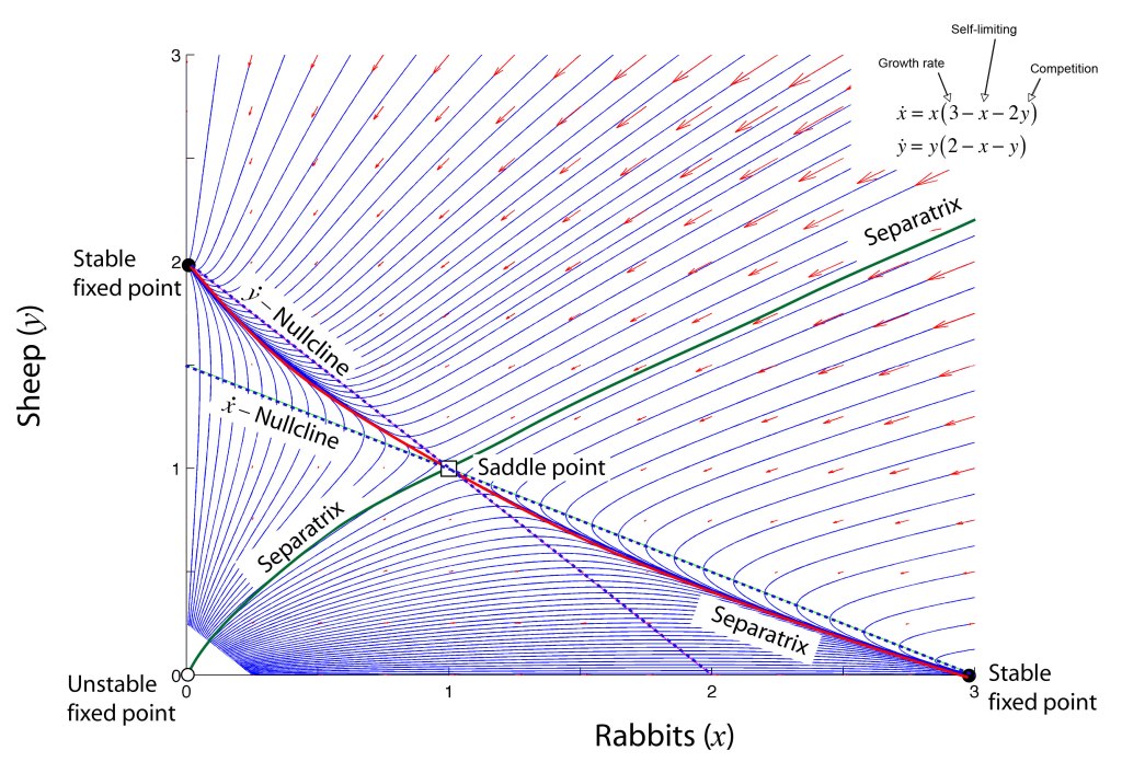
Voters in a political party are not too different from species in an ecosystem. There are many population dynamics models of things like rabbit and sheep that seek to understand the steady-state solutions when two species vie for the same feedstock (or two parties vie for the same votes). Depending on reproduction rates and competition payoff, one species can often drive the other species to extinction. Yet with fairly small modifications of the model parameters, it is often possible to find a steady-state solution in which both species live in harmony. This is a symbiotic solution to the population dynamics, perhaps because the rabbits help fertilize the grass for the sheep to eat, and the sheep keep away predators for the rabbits.
There are two interesting features to such a symbiotic population-dynamics model. First, because there is a stable steady-state solution, if there is a perturbation of the populations, for instance if the rabbits are culled by the farmer, then the two populations will slowly relax back to the original steady-state solution. For this reason, this solution is called a “stable fixed point”. Deviations away from the steady-state values experience an effective “restoring force” that moves the population values back to the fixed point. The second feature of these models is that the steady state values depend on the parameters of the model. Small changes in the model parameters then cause small changes in the steady-state values. In this sense, this stable fixed point is not fundamental–it depends on the parameters of the model.
But there are dynamical models which do have a stability that maintains steady values even as the model parameters shift. These models have negative feedback, like many dynamical systems, but if the negative feedback is connected to winner-take-all outcomes of game theory, then a robustly stable fixed point can emerge at precisely the threshold where such a winner would take all.
The Replicator Equation
The replicator equation provides a simple model for competing populations [2]. Despite its simplicity, it can model surprisingly complex behavior. The central equation is a simple growth model
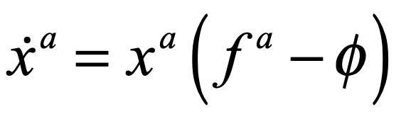
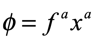
where the growth rate depends on the fitness fa of the a-th species relative to the average fitness φ of all the species. The fitness is given by
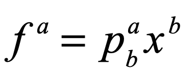
where pab is the payoff matrix among the different species (implicit Einstein summation applies). The fitness is frequency dependent through the dependence on xb. The average fitness is
This model has a zero-sum rule that keeps the total population constant. Therefore, a three-species dynamics can be represented on a two-dimensional “simplex” where the three vertices are the pure populations for each of the species. The replicator equation can be applied easily to a three-party system, one simply defines a payoff matrix that is used to define the fitness of a party relative to the others.
The Nonlinear Dynamics of Presidential Elections
Here we will consider the replicator equation with three political parties (Democratic, Republican and Libertarian). Even though the third party is never a serious contender, the extra degree of freedom provided by the third party helps to stabilize the dynamics between the Democrats and the Republicans.
It is already clear that an essentially symbiotic relationship is at play between Democrats and Republicans, because the elections are roughly 50/50. If this were not the case, then a winner-take-all dynamic would drive virtually everyone to one party or the other. Therefore, having 100% Democrats is actually unstable, as is 100% Republicans. When the populations get too far out of balance, they get too monolithic and too inflexible, then defections of members will occur to the other parties to rebalance the system. But this is just a general trend, not something that can explain the nearly perfect 50/50 vote of the 2020 election.
To create the ultra-stable fixed point at 50/50 requires an additional contribution to the replicator equation. This contribution must create a type of toggle switch that depends on the winner-take-all outcome of the election. If a Democrat wins 51% of the vote, they get 100% of the Oval Office. This extreme outcome then causes a back action on the electorate who is always afraid when one party gets too much power.
Therefore, there must be a shift in the payoff matrix when too many votes are going one way or the other. Because the winner-take-all threshold is at exactly 50% of the vote, this becomes an equilibrium point imposed by the payoff matrix. Deviations in the numbers of voters away from 50% causes a negative feedback that drives the steady-state populations back to 50/50. This means that the payoff matrix becomes a function of the number of voters of one party or the other. In the parlance of nonlinear dynamics, the payoff matrix becomes frequency dependent. This goes one step beyond the original replicator equation where it was the population fitness that was frequency dependent, but not the payoff matrix. Now the payoff matrix also becomes frequency dependent.
The frequency-dependent payoff matrix (in an extremely simple model of the election dynamics) takes on negative feedback between two of the species (here the Democrats and the Republicans). If these are the first and third species, then the payoff matrix becomes
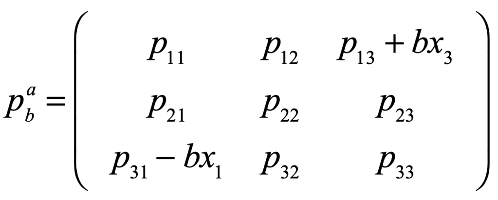
where the feedback coefficient is
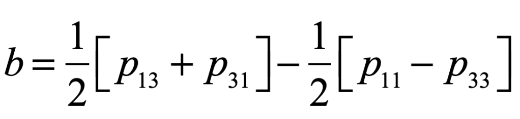
and where the population dependences on the off-diagonal terms guarantee that, as soon as one party gains an advantage, there is defection of voters to the other party. This establishes a 50/50 balance that is maintained even when the underlying parameters would predict a strongly asymmetric election.
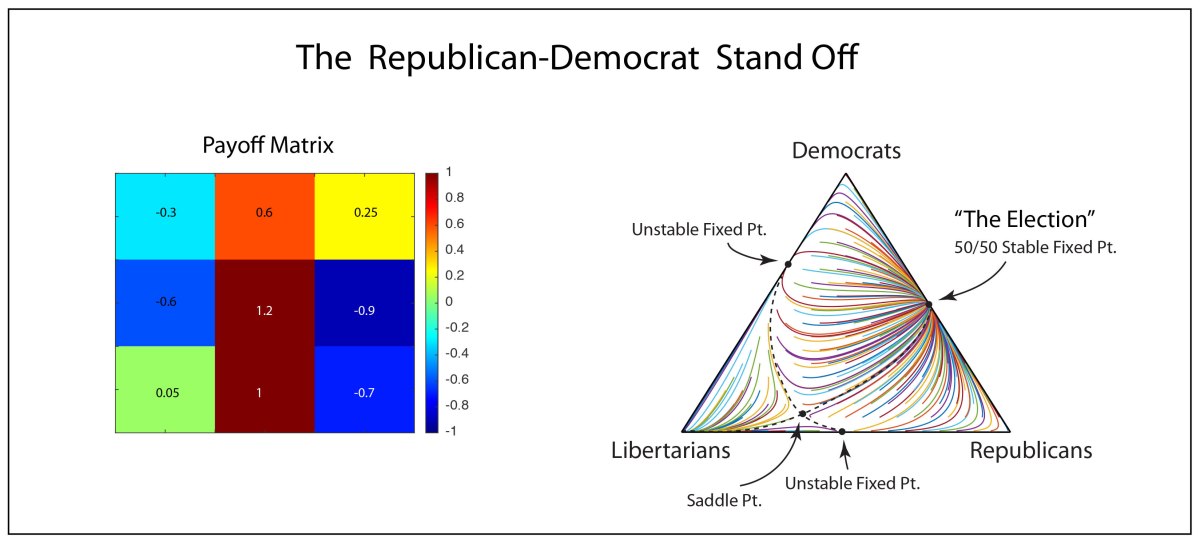
For instance, look at the dynamics in Fig. 2. For this choice of parameters, the replicator model predicts a 75/25 win for the democrats. However, when the feedback is active, it forces the 50/50 outcome, despite the underlying advantage for the original parameters.
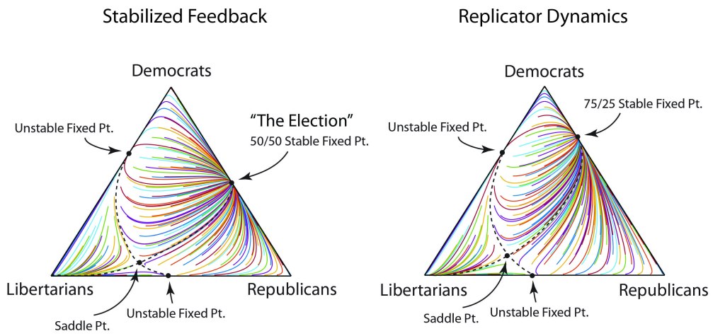
There are several interesting features in this model. It may seem that the Libertarians are irrelevant because they never have many voters. But their presence plays a surprisingly important role. The Libertarians tend to stabilize the dynamics so that neither the democrats nor the republicans would get all the votes. Also, there is a saddle point not too far from the pure Libertarian vertex. That Libertarian vertex is an attractor in this model, so under some extreme conditions, this could become a one-party system…maybe not Libertarian in that case, but possibly something more nefarious, of which history can provide many sad examples. It’s a word of caution.
Disclaimers and Caveats
No attempt has been made to actually mode the US electorate. The parameters in the modified replicator equations are chosen purely for illustration purposes. This model illustrates a concept — that feedback in the payoff matrix can create an ultra-stable fixed point that is insensitive to changes in the underlying parameters of the model. This can possibly explain why so many of the US presidential elections are so tight.
Someone interested in doing actual modeling of US elections would need to modify the parameters to match known behavior of the voting registrations and voting records. The model presented here assumes a balanced negative feedback that ensures a 50/50 fixed point. This model is based on the aversion of voters to too much power in one party–an echo of the libertarian tradition in the country. A more sophisticated model would yield the fixed point as a consequence of the dynamics, rather than being a feature assumed in the model. In addition, nonlinearity could be added that would drive the vote off of the 50/50 point when the underlying parameters shift strongly enough. For instance, the 2008 election was not a close one, in part because the strong positive character of one of the candidates galvanized a large fraction of the electorate, driving the dynamics away from the 50/50 balance.
References
[1] D. D. Nolte, Introduction to Modern Dynamics: Chaos, Networks, Space and Time (Oxford University Press, 2019) 2nd Edition.
[2] Nowak, M. A. (2006). Evolutionary Dynamics: Exploring the Equations of Life. Cambridge, Mass., Harvard University Press.