Machine learning is characterized, more than by any other aspect, by the high dimensionality of the data spaces it seeks to find patterns in. Hence, one of the principle functions of machine learning is to reduce the dimensionality of the data to lower dimensions—a process known as dimensionality reduction.
There are two driving reasons to reduce the dimensionality of data:
First, typical dimensionalities faced by machine learning problems can be in the hundreds or thousands. Trying to visualize such high dimensions may sound mind expanding, but it is really just saying that a data problem may have hundreds or thousands of different data entries for a single event. And many, or even most, of those entries may not be independent. While many others may be pure noise—or at least not relevant to the pattern. Deep learning dimensionality reduction seeks to find the dependences—many of them nonlinear and non-single-valued (non-invertible)—and to reject the noise channels.
Second, the geometry of high dimension is highly unintuitive. Many of the things we take for granted in our pitifully low dimension of 3 (or 4 if you include time) just don’t hold in high dimensions. For instance, in very high dimensions almost all random vectors in a hyperspace are orthogonal, and almost all random unit vectors in the hyperspace are equidistant. Even the topology of landscapes in high dimensions is unintuitive—there are far more mountain ridges than mountain peaks—with profound consequences for dynamical processes such as random walks (see my Blog on a Random Walk in 10 Dimensions). In fact, we owe our evolutionary existence to this effect! Therefore, deep dimensionality reduction is a way to bring complex data down to a dimensionality where our intuition can be applied to “explain” the data.
But what is a dimension? And can you find the “right” dimensionality when performing dimensionality reduction? Once again, our intuition struggles with these questions, as first discovered by a nineteenth-century German mathematician whose mind-expanding explorations of the essence of different types of infinity shattered the very concept of dimension.
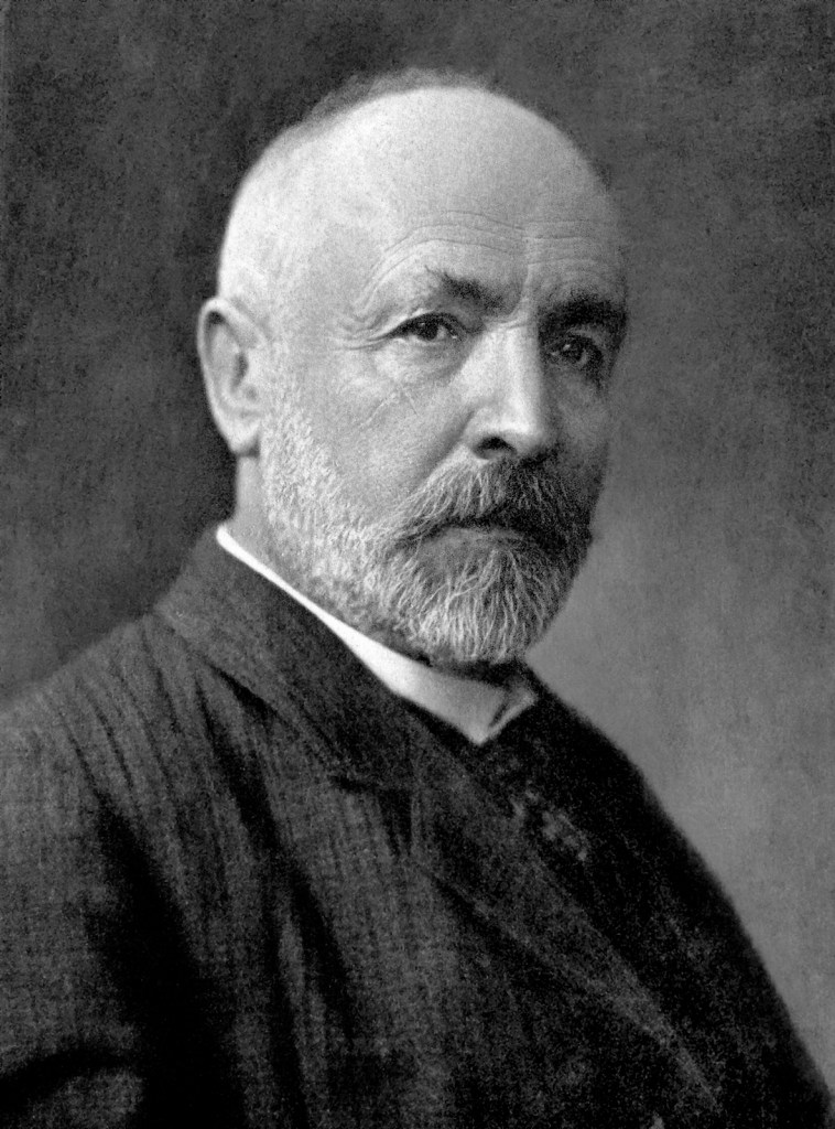
George Cantor
Georg Cantor (1845 – 1918) was born in Russia, and the family moved to Germany while Cantor was still young. In 1863, he enrolled at the University of Berlin where he sat on lectures by Weierstrass and Kronecker. He received his doctorate in 1867 and his Habilitation in 1869, moving into a faculty position at the University of Halle and remaining there for the rest of his career. Cantor published a paper early in 1872 on the question of whether the representation of an arbitrary function by a Fourier series is unique. He had found that even though the series might converge to a function almost everywhere, there surprisingly could still be an infinite number of points where the convergence failed. Originally, Cantor was interested in the behavior of functions at these points, but his interest soon shifted to the properties of the points themselves, which became his life’s work as he developed set theory and transfinite mathematics.
In 1878, in a letter to his friend Richard Dedekind, Cantor showed that there was a one-to-one correspondence between the real numbers and the points in any n-dimensional space. He was so surprised by his own result that he wrote to Dedekind “I see it, but I don’t believe it.” Previously, the ideas of a dimension, moving in a succession from one (a line) to two (a plane) to three (a volume) had been absolute. However, with his newly-discovered mapping, the solid concepts of dimension and dimensionality began to dissolve. This was just the beginning of a long history of altered concepts of dimension (see my Blog on the History of Fractals).
Mapping Two Dimensions to One
Cantor devised a simple mapping that is at once obvious and subtle. To take a specific example of mapping a plane to a line, one can consider the two coordinate values (x,y) both with a closed domain on [0,1]. Each can be expressed as a decimal fraction given by
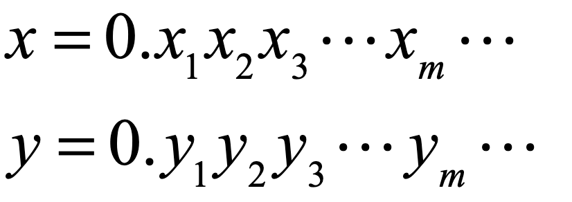
These two values can be mapped to a single value through a simple “ping-pong” between the decimal digits as
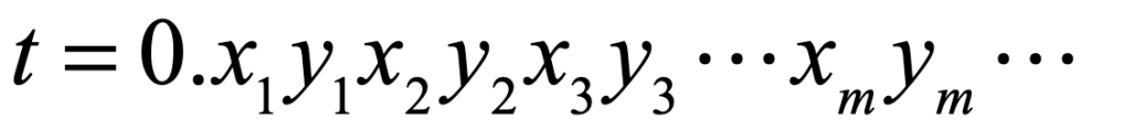
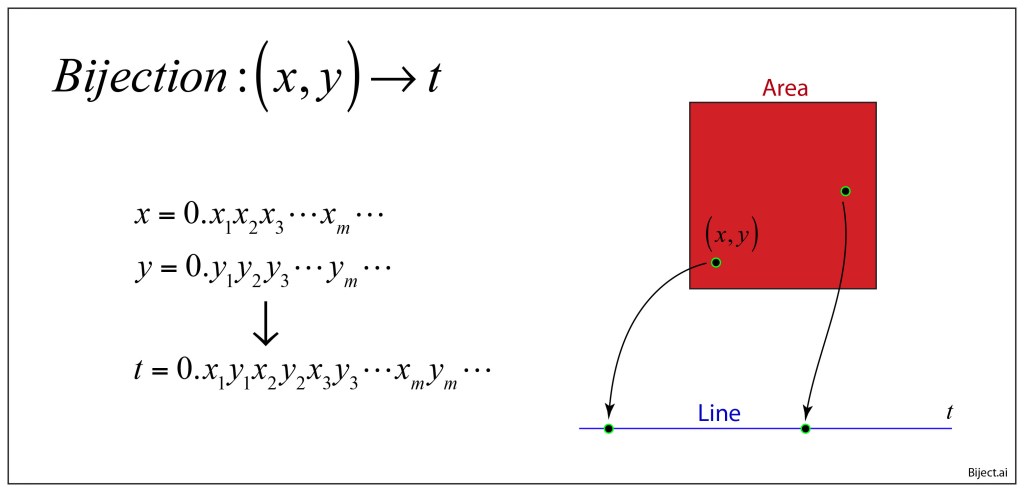
If x and y are irrational, then this presents a simple mapping of a pair of numbers (two-dimensional coordinates) to a single number. In this way, the special significance of two dimensions relative to one dimension is lost. In terms of set theory nomenclature, the cardinality of the two-dimensional R2 is the same as for the one-dimensions R.
Nonetheless, intuition about dimension still has it merits, and a subtle aspect of this mapping is that it contains discontinuities. These discontinuities are countably infinite, but they do disrupt any smooth transformation from 2D to 1D, which is where the concepts of intrinsic dimension are hidden. The topological dimension of the plane is clearly equal to 2, and that of the line is clearly equal to 1, determined by the dimensionality D+1 of cuts that are required to separate the sets. The area is separated by a D = 1 line, while the line is separated by a D= 0 point.
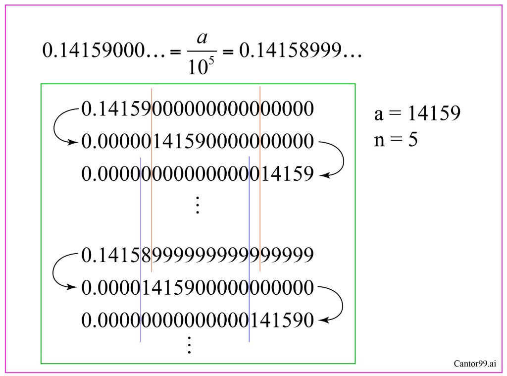
While the discontinuities help preserve the notions of dimension, and they are countably infinite (with the cardinality of the rational numbers), they pertain merely to the representation of number by decimals. As an example, in decimal notation for a number a = 14159/105, one has two equivalent representations
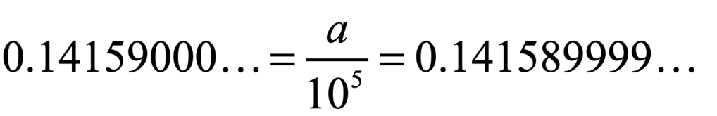
trailing either infinitely many 0’s or infinitely many 9’s. Despite the fact that these representations point to the same number, when it is used as one of the pairs in the bijection of Fig. 1, it produces two distinctly different numbers of t in R. Fortunately, there is a way to literally sweep this under the rug. Any time one retrieves a number that has repeating 0’s or 9’s, simply sweep it to the right it by dividing by a power of 10 to a region of trailing zeros for a different number, call it b, as in Fig. 2. The shifted version of a will not overlap with the number b, because b also ends in repeating 0’s or 9’s and so is swept farther to the right, and so on to infinity, so none of these numbers overlap, each is distinct, and the mapping becomes what is known as a bijection with one-to-one correspondence.
Space-Filling Curves
When the peripatetic mathematician Guiseppe Peano learned of Cantor’s result for the mapping of 2D to 1D, he sought to demonstrate the correspondence geometrically, and he constructed a continuous curve that filled space, publishing the method in Sur une courbe, qui remplit toute une aire plane [1] in 1890. The construction of Peano’s curve proceeds by taking a square and dividing it into 9 equal sub squares. Lines connect the centers of each of the sub squares. Then each sub square is divided again into 9 sub squares whose centers are all connected by lines. At this stage, the original pattern, repeated 9 times, is connected together by 8 links, forming a single curve. This process is repeated infinitely many times, resulting in a curve that passes through every point of the original plane square. In this way, a line is made to fill a plane. Where Cantor had proven abstractly that the cardinality of the real numbers was the same as the points in n-dimensional space, Peano created a specific example.
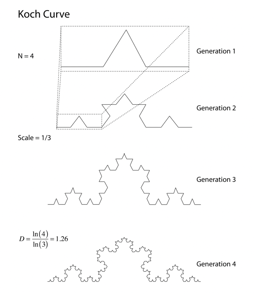
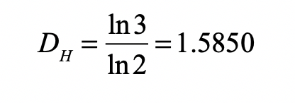
This was followed quickly by another construction, invented by David Hilbert in 1891, that divided the square into four instead of nine, simplifying the construction, but also showing that such constructions were easily generated [2]. The space-filling curves of Peano and Hilbert have the extreme properties that a one-dimensional curve approaches every point in a two-dimensional space. These curves have topological dimensionality of 1D and a fractal dimensionality of 2D.

A One-Dimensional Deep Discrete Encoder for MNIST
When performing dimensionality reduction in deep learning it is tempting to think that there is an underlying geometry to the data—as if they reside on some submanifold of the original high-dimensional space. While this can be the case (for which dimensionality reduction is called deep metric learning) more often there is no such submanifold. For instance, when there is a highly conditional nature to the different data channels, in which some measurements are conditional on the values of other measurements, then there is no simple contiguous space that supports the data.
It is also tempting to think that a deep learning problem has some intrinsic number of degrees of freedom which should be matched by the selected latent dimensionality for the dimensionality reduction. For instance, if there are roughly five degrees of freedom buried within a complicated data set, then it is tempting to believe that the appropriate latent dimensionality also should be chosen to be five. But this also is missing the mark.
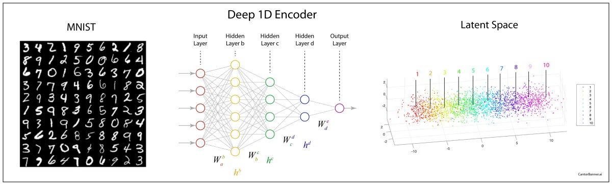
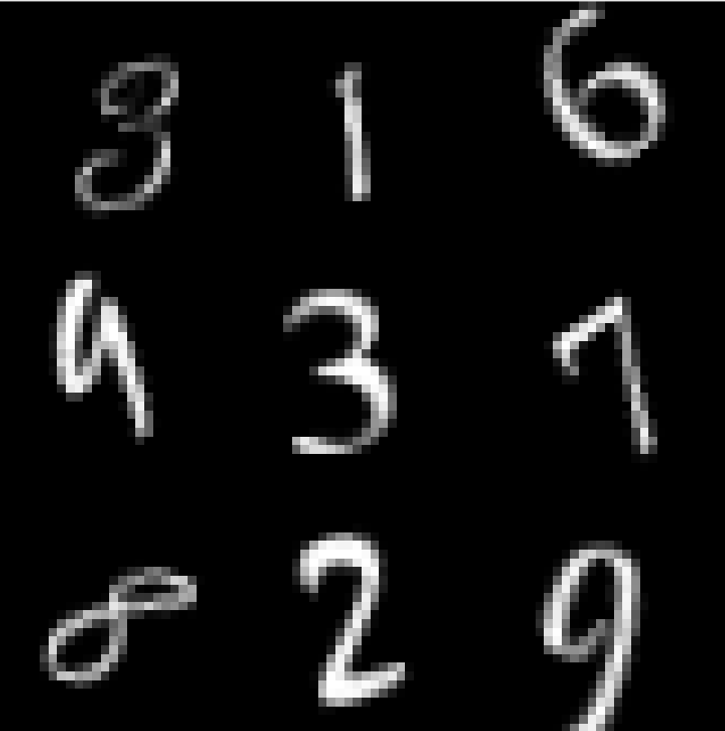
Take, for example, the famous MNIST data set of hand-written digits from 0 to 9. Each digit example is contained in a 28-by28 two-dimensional array that is typically flattened to a 784-element linear vector that locates that single digit example within a 784-dimensional space. The goal is to reduce the dimensionality down to a manageable number—but what should the resulting latent dimensionality be? How many degrees of freedom are involved in writing digits? Furthermore, given that there are ten classes of digits, should the chosen dimensionality of the latent space be related to the number of classes?
To illustrate that the dimensionality of the latent space has little to do with degrees of freedom or the number of classes, let’s build a simple discrete encoder that encodes the MNIST data set to the one-dimensional line—following Cantor.
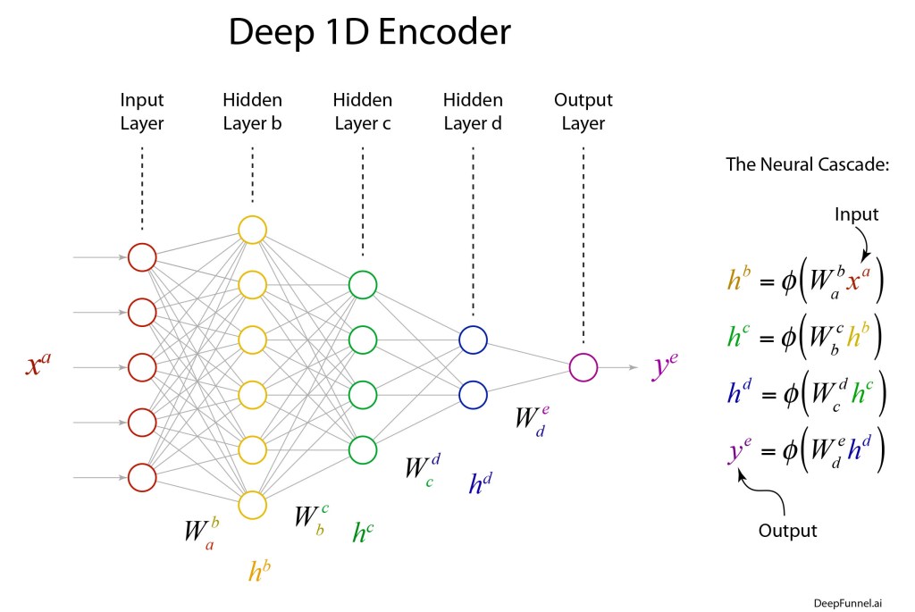
The deep network of the encoder can have a simple structure that terminates with a single neuron that has a piece-wise linear output. The objective function (or loss function) measures the squared distances of the outputs of the single neuron, after transformation by the network, to the associated values 0 to 9. And that is it! Train the network by minimizing the loss function.
The results of the linear encoder are shown in Fig. 6 (the transverse directions are only for ease of visualization…the classification is along the long axis). The different dots are specific digits, and the colors are the digit value. There is a clear trend from 1 through 10, although with this linear encoder there is substantial overlap among the point clouds.
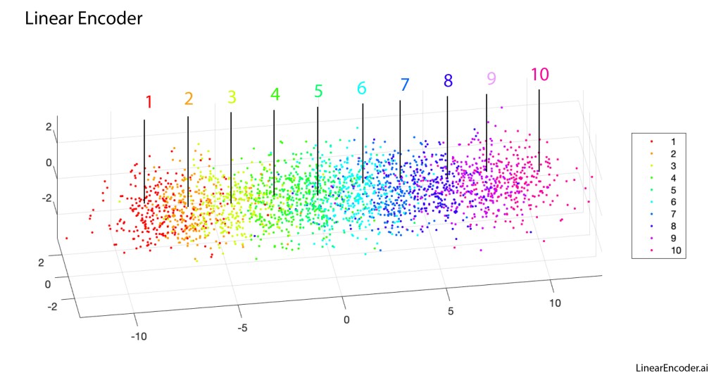
Despite appearances, this one-dimensional discrete line encoder is NOT a form of regression. There is no such thing as 1.5 as the average of a 1-digit and a 2-digit. And 5 is not the average of a 4-digit and a 6-digit. The digits are images that have no intrinsic numerical value. Therefore, this one-dimensional encoder is highly discontinuous, and intuitive ideas about intrinsic dimension for continuous data remain secure.
Summary
The purpose of this Blog (apart from introducing Cantor and his ideas on dimension theory) was to highlight a key question of dimensionality reduction in representation theory: What is the intrinsic dimensionality of a dataset? The answer, in the case of discrete classes, is that there is no intrinsic dimensionality. Having 1 degree of freedom or 10 degrees of freedom, i.e. latent dimensionalities of 1 or 10, is mostly irrelevant. In ideal cases, one is just as good as the other.
On the other hand, for real-world data with its inevitable variability and finite variance, there can be reasons to choose one latent dimensionality over another. In fact, the “best” choice of dimensionality is one less than the number of classes. For instance, in the case of MNIST with its 10 classes, that is a 9-dimensional latent space. The reason this is “best” has to do with the geometry of high-dimensional simplexes, which will be the topic of a future Blog.
By David D. Nolte, June 20, 2022
[1] G.Peano: Sur une courbe, qui remplit toute une aire plane. Mathematische Annalen 36 (1890), 157–160.
[2] D. Hilbert, “Uber die stetige Abbildung einer Linie auf ein Fllichenstilck,” Mathemutische Anna/en, vol. 38, pp. 459-460, (1891)