Paul Lévy’s Black Swan: The Physics of Outliers

The Black Swan was a mythical beast invented by the Roman poet Juvenal as a metaphor for things that are so rare they can only be imagined.  His quote goes “rara avis in terris nigroque simillima cygno” (a rare bird in the lands and very much like a black swan).

Imagine the shock, then, when the Dutch explorer Willem de Vlamingh first saw black swans in Australia in 1697.  The metaphor morphed into a new use, meaning when a broadly held belief (the impossibility of black swans) is refuted by a single new observation. 

For instance, in 1870 the biologist Thomas Henry Huxley, known as “Darwin’s Bulldog” for his avid defense of Darwin’s theories, delivered a speech in Liverpool, England, where he was quoted in Nature magazine as saying,

… the great tragedy of Science—the slaying of a beautiful hypothesis by an ugly fact

This quote has been picked up and repeated over the years in many different contexts. 

One of those contexts applies to the fate of a beautiful economic theory, proposed by Fischer Black and Myron Scholes in 1973, as a way to make the perfect hedge on Wall Street, purportedly risk free, yet guaranteeing a positive return in spite of the ups-and-downs of stock prices.  Scholes and Black launched an investment company in 1994 to cash in on this beautiful theory, returning an unbelievable 40% on investment.  Black died in 1995, but Scholes was awarded the Nobel Prize in Economics in 1997.  The next year, the fund went out of business.  The ugly fact that flew in the face of Black-Scholes was the Black Swan.

The Black Swan

A Black Swan is an outlier measurement that occurs in a sequence of data points.  Up until the Black Swan event, the data points behave normally, following the usual statistics we have all come to expect, maybe a Gaussian distribution or some other form of exponential that dominate most variable phenomena.

Fig. An Australian Black Swan (Wikipedia).

But then a Black Swan occurs.  It has a value so unexpected, and so unlike all the other measurements, that it is often assumed to be wrong and possibly even thrown out because it screws up the otherwise nice statistics.  That single data point skews averages and standard deviations in non-negligible ways.  The response to such a disturbing event is to take even more data to let the averages settle down again … until another Black Swan hits and again skews the mean value. However, such outliers are often not spurious measurements but are actually a natural part of the process. They should not, and can not, be thrown out without compromising the statistical integrity of the study.

This outlier phenomenon came to mainstream attention when the author Nassim Nicholas Taleb, in his influential 2007 book, The Black Swan: The Impact of the Highly Improbable, pointed out that it was a central part of virtually every aspect of modern life, whether in business, or the development of new technologies, or the running of elections, or the behavior of financial markets.  Things that seemed to be well behaved … a set of products, or a collective society, or a series of governmental policies … are suddenly disrupted by a new invention, or a new law, or a bad Supreme Court decision, or a war, or a stock-market crash.

As an illustration, let’s see where Black-Scholes went wrong.

The Perfect Hedge on Wall Street?

Fischer Black (1938 – 1995) was a PhD advisor’s nightmare.  He had graduated as an undergraduate physics major from Harvard in 1959, but then switched to mathematics for graduate school, then switched to computers, then switched again to artificial intelligence, after which he was thrown out of the graduate program at Harvard for having a serious lack of focus.  So he joined the RAND corporation, where he had time to play with his ideas, eventually approaching Marvin Minsky at MIT, who helped guide him to an acceptable thesis that he was allowed to submit to the Harvard program for his PhD in applied mathematics.  After that, he went to work in financial markets.

His famous contribution to financial theory was the Black-Scholes paper of 1973 on “The Pricing of Options and Corporate Liabilities” co-authored with Byron Scholes.   Hedging is a venerable tradition on Wall Street.  To hedge means that a broker sells an option (to purchase a stock at a given price at a later time) assuming that the stock will fall in value (selling short), and then buys, as insurance against the price rising, a number of shares of the same asset (buying long).  If the broker balances enough long shares with enough short options, then the portfolio’s value is insulated from the day-to-day fluctuations of the value of the underlying asset. 

This type of portfolio is one example of a financial instrument called a derivative.  The name comes from the fact that the value of the portfolio is derived from the values of the underlying assets.  The challenge with derivatives is finding their “true” value at any time before they mature.  If a broker knew the “true” value of a derivative, then there would be no risk in buying and selling derivatives.

To be risk free, the value of the derivative needs to be independent of the fluctuations.  This appears at first to be a difficult problem, because fluctuations are random and cannot be predicted.  But the solution actually relies on just this condition of randomness.  If the random fluctuations in stock prices are equivalent to a random walk superposed on the average rate of return, then perfect hedges can be constructed with impunity.

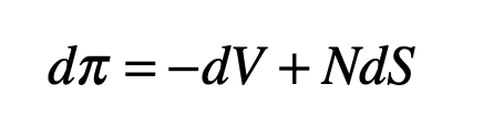
To make a hedge on an underlying asset, create a portfolio by selling one call option (selling short) and buying a number N shares of the asset (buying long) as insurance against the possibility that the asset value will rise.  The value of this portfolio is

If the number N is chosen correctly, then the short and long positions will balance, and the portfolio will be protected from fluctuations in the underlying asset price.  To find N, consider the change in the value of the portfolio as the variables fluctuate

and use an elegant result known as Ito’s Formula (a stochastic differential equation that includes the effects of a stochastic variable) to yield

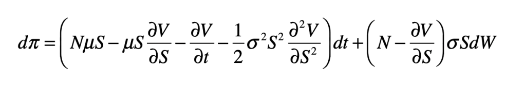
Note that the last term contains the fluctuations, expressed using the stochastic term dW (a random walk).  The fluctuations can be zeroed-out by choosing
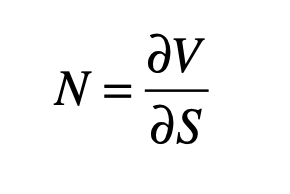
which yields

The important observation about this last equation is that the stochastic function W has disappeared.  This is because the fluctuations of the N share prices balance the fluctuations of the short option. 

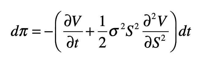
When a broker buys an option, there is a guaranteed rate of return r at the time of maturity of the option which is set by the value of a risk-free bond.  Therefore, the price of a perfect hedge must increase with the risk-free rate of return.  This is
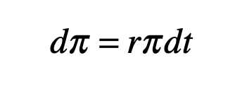
or

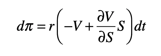
Equating the two equations gives

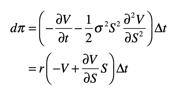
Simplifying, this leads to a partial differential equation for V(S,t)

The Black-Scholes equation is a partial differential equation whose solution, given the boundary conditions and time, defines the “true” value of the derivative and determines how many shares to buy at t = 0 at a specified guaranteed return rate r (or, alternatively, stating a specified stock price S(T) at the time of maturity T of the option).  It is a diffusion equation that incorporates the diffusion of the stock price with time.  If the derivative is sold at any time t prior to maturity, when the stock has some value S, then the value of the derivative is given by V(S,t) as the solution to the Black-Scholes equation [1].

One of the interesting features of this equation is the absence of the mean rate of return μ of the underlying asset.  This means that any stock of any value can be considered, even if the rate of return of the stock is negative!  This type of derivative looks like a truly risk-free investment.  You would be guaranteed to make money even if the value of the stock falls, which may sound too good to be true…which of course it is. 

Black, Scholes and Merton. Sholes and Merton were winners of the 1997 Nobel Prize in Economics.

The success (or failure) of derivative markets depends on fundamental assumptions about the stock market.  These include that it would not be subject to radical adjustments or to panic or irrational exuberance, i.i. Black-Swan events, which is clearly not the case.  Just think of booms and busts.  The efficient and rational market model, and ultimately the Black-Scholes equation, assumes that fluctuations in the market are governed by Gaussian random statistics.  However, there are other types of statistics that are just as well behaved as the Gaussian, but which admit Black Swans.

Stable Distributions: Black Swans are the Norm

When Paul Lévy (1886 – 1971) was asked in 1919 to give three lectures on random variables at the École Polytechnique, the mathematical theory of probability was just a loose collection of principles and proofs. What emerged from those lectures was a lifetime of study in a field that now has grown to become one of the main branches of mathematics. He had a distinguished and productive career, although he struggled to navigate the anti-semitism of Vichy France during WWII. His thesis advisor was the famous Jacques Hadamard and one of his students was the famous Benoit Mandelbrot.

Lévy wrote several influential textbooks that established the foundations of probability theory, and his name has become nearly synonymous with the field. One of his books was on the theory of the addition of random variables [2] in which he extended the idea of a stable distribution.

Fig. Paul Lévy in his early years. Les Annales des Mines

In probability theory, a class of distributions are called stable if a sum of two independent random variables that come from a distribution have the same distribution.  The normal (Gaussian) distribution clearly has this property because the sum of two normally distributed independent variables is also normally distributed.  The variance and possibly the mean may be different, but the functional form is still Gaussian. 

Fig. A look at Paul Lévy’s theory of the addition of random variables.

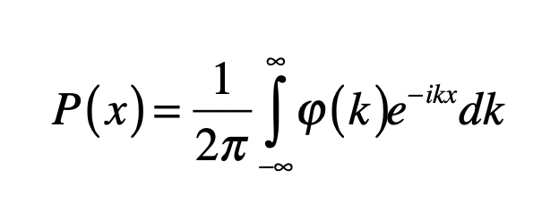
The general form of a probability distribution can be obtained by taking a Fourier transform as

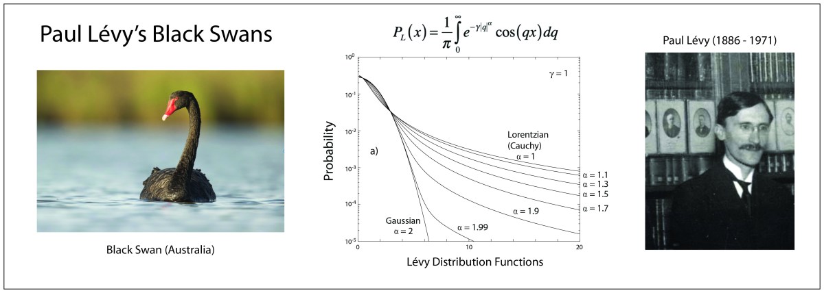
where φ  is known as the characteristic function of the probability distribution.  A special case of a stable distribution is the Lévy symmetric stable distribution obtained as

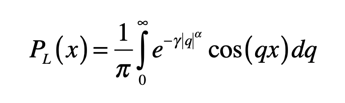
which is parameterized by α and γ.  The characteristic function in this case is called a stretched exponential with the length scale set by the parameter γ. 

The most important feature of the Lévy distribution is that it has a power-law tail at large values.  For instance, the special case of the Lévy distribution for α = 1 is the Cauchy distribution for positive values x given by

which falls off at large values as x-(α+1). The Cauchy distribution is normalizable (probabilities integrate to unity) and has a characteristic scale set by γ, but it has a divergent mean value, violating the central limit theorem [3].  For distributions that satisfy the central limit theorem, increasing the number of samples from the distribution allows the mean value to converge on a finite value.  However, for the Cauchy distribution increasing the number of samples increases the chances of obtaining a black swan, which skews the mean value, and the mean value diverges to infinity in the limit of an infinite number of samples. This is why the Cauchy distribution is said to have a “heavy tail” that contains rare, but large amplitude, outlier events that keep shifting the mean.

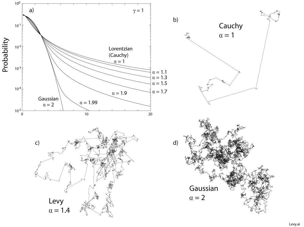
Examples of Levy stable probability distribution functions are shown below for a range between α = 1 (Cauchy) and α = 2 (Gaussian).  The heavy tail is seen even for the case α = 1.99 very close to the Gaussian distribution.  Examples of two-dimensional Levy walks are shown in the figure for α = 1, α = 1.4 and α = 2.  In the case of the Gaussian distribution, the mean-squared displacement is well behaved and finite.  However, for all the other cases, the mean-squared displacement is divergent, caused by the large path lengths that become more probable as α approaches unity.

Fig. Symmetric Lévy distribution functions for a range of parameters α from α = 1 (Cauchy) to α = 2 (Gaussian). Levy flights for α < 2 have a run-and-tumble behavior that is often seen in bacterial motion.

The surprising point of the Lévy probability distribution functions is how common they are in natural phenomena. Heavy Lévy tails arise commonly in almost any process that has scale invariance. Yet as students, we are virtually shielded from them, as if Poisson and Gaussian statistics are all we need to know, but ignorance is not bliss. The assumption of Gaussian statistics is what sank Black-Scholes.

Scale-invariant processes are often consequences of natural cascades of mass or energy and hence arise as neutral phenomena. Yet there are biased phenomena in which a Lévy process can lead to a form of optimization. This is the case for Lévy random walks in biological contexts.

Lévy Walks

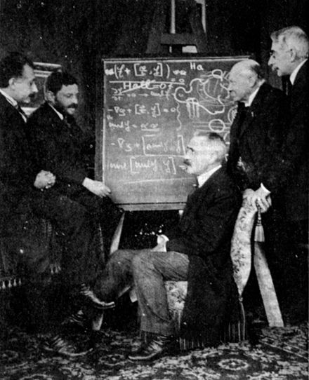
The random walk is one of the cornerstones of statistical physics and forms the foundation for Brownian motion which has a long and rich history in physics. Einstein used Brownian motion to derive his famous statistical mechanics equation for diffusion, proving the existence of molecular matter. Jean Perrin won the Nobel prize for his experimental demonstrations of Einstein’s theory. Paul Langevin used Brownian motion to introduce stochastic differential equations into statistical physics. And Lévy used Brownian motion to illustrate applications of mathematical probability theory, writing his last influential book on the topic.

Most treatments of the random walk assume Gaussian or Poisson statistics for the step length or rate, but a special form of random walk emerges when the step length is drawn from a Lévy distribution. This is a Lévy random walk, also named a “Lévy Flight” by Benoit Mandelbrot (Lévy’s student) who studied its fractal character.

Originally, Lévy walks were studied as ideal mathematical models, but there have been a number of discoveries in recent years in which Lévy walks have been observed in the foraging behavior of animals, even in the run-and-tumble behavior of bacteria, in which rare long-distance runs are followed by many local tumbling excursions. It has been surmised that this foraging strategy allows an animal to optimally sample randomly-distributed food sources. There is evidence of Lévy walks of molecules in intracellular transport, which may arise from random motions within the crowded intracellular neighborhood. A middle ground has also been observed [4] in which intracellular organelles and vesicles may take on a Lévy walk character as they attach, migrate, and detach from molecular motors that drive them along the cytoskeleton.

By David D. Nolte, Feb. 8, 2023


Selected Bibliography

Paul Lévy, Calcul des probabilités (Gauthier-Villars, Paris, 1925).

Paul Lévy, Théorie de l’addition des variables aléatoires (Gauthier-Villars, Paris, 1937).

Paul Lévy, Processus stochastique et mouvement brownien (Gauthier-Villars, Paris, 1948).

R. Metzler, J. Klafter, The random walk’s guide to anomalous diffusion: a fractional dynamics approach. Physics Reports-Review Section Of Physics Letters 339, 1-77 (2000).

J. Klafter, I. M. Sokolov, First Steps in Random Walks : From Tools to Applications.  (Oxford University Press, 2011).

F. Hoefling, T. Franosch, Anomalous transport in the crowded world of biological cells. Reports on Progress in Physics 76,  (2013).

V. Zaburdaev, S. Denisov, J. Klafter, Levy walks. Reviews of Modern Physics 87, 483-530 (2015).


References

[1]  Black, Fischer; Scholes, Myron (1973). “The Pricing of Options and Corporate Liabilities”. Journal of Political Economy. 81 (3): 637–654.

[2] P. Lévy, Théorie de l’addition des variables aléatoire (1937)

[3] The central limit theorem holds if the mean value of a number of N samples converges to a stable value as the number of samples increases to infinity.

[4] H. Choi, K. Jeong, J. Zuponcic, E. Ximenes, J. Turek, M. Ladisch, D. D. Nolte, Phase-Sensitive Intracellular Doppler Fluctuation Spectroscopy. Physical Review Applied 15, 024043 (2021).

Random Walks with Paul Langevin: Stochastic Dynamics

One of the most important conclusions from chaos theory is that not all random-looking processes are actually random.  In deterministic chaos, structures such as strange attractors are not random at all but are fractal structures determined uniquely by the dynamics.  But sometimes, in nature, processes really are random, or at least have to be treated as such because of their complexity.  Brownian motion is a perfect example of this.  At the microscopic level, the jostling of the Brownian particle can be understood in terms of deterministic momentum transfers from liquid atoms to the particle.  But there are so many liquid particles that their individual influences cannot be directly predicted.  In this situation, it is more fruitful to view the atomic collisions as a stochastic process with well-defined physical parameters and then study the problem statistically. This is what Einstein did in his famous 1905 paper that explained the statistical physics of Brownian motion.

Then there is the middle ground between deterministic mechanics and stochastic mechanics, where complex dynamics gains a stochastic component. This is what Paul Langevin did in 1908 when he generalized Einstein.

Paul Langevin

Paul Langevin (1872 – 1946) had the fortune to stand at the cross-roads of modern physics, making key contributions, while serving as a commentator expanding on the works of the giants like Einstein and Lorentz and Bohr.  He was educated at the École Normale Supérieure and at the Sorbonne with a year in Cambridge studying with J. J. Thompson.  At the Sorbonne he worked in the laboratory of Jean Perrin (1870 – 1942) who received the Nobel Prize in 1926 for the experimental work on Brownian motion that had set the stage for Einstein’s crucial analysis of the problem confirming the atomic nature of matter. 

Langevin received his PhD in 1902 on the topic of x-ray ionization of gases and was appointed as a lecturer at the College de France to substitute in for Éleuthère Mascart (who was an influential French physicist in optics).  In 1905 Langevin published several papers that delved into the problems of Lorentz contraction, coming very close to expressing the principles of relativity.  This work later led Einstein to say that, had he delayed publishing his own 1905 paper on the principles of relativity, then Langevin might have gotten there first [1].

Fig. 1 From left to right: Albert Einstein, Paul Ehrenfest, Paul Langevin (seated), Kamerlingh Onnes, and Pierre Weiss

Also in 1905, Langevin published his most influential work, providing the theoretical foundations for the physics of paramagnetism and diamagnetism.  He was working closely with Pierre Curie whose experimental work on magnetism had established the central temperature dependence of the phenomena.  Langevin used the new molecular model of matter to derive the temperature dependence as well as the functional dependence on magnetic field.  One surprising result was that only the valence electrons, moving relativistically, were needed to contribute to the molecular magnetic moment.  This later became one of the motivations for Bohr’s model of multi-electron atoms.

Langevin suffered personal tragedy during World War II when the Vichy government arrested him because of his outspoken opposition to fascism.  He was imprisoned and eventually released to house arrest.  In 1942, his son-in-law was executed by the Nazis, and in 1943 his daughter was sent to Auschwitz.  Fearing for his own life, Langevin escaped to Switzerland.  He returned shortly after the liberation of Paris and was joined after the end of the war by his daughter who had survived Auschwitz and later served in the Assemblée Consultative as a communist member.  Langevin passed away in 1946 and received a national funeral.  His remains lie today in the Pantheon.

The Langevin Equation

In 1908, Langevin realized that Einstein’s 1905 theory on Brownian motion could be simplified while at the same time generalized.  Langevin introduced a new quantity into theoretical physics—the stochastic force [2].  With this new theoretical tool, he was able to work with diffusing particles in momentum space as dynamical objects with inertia buffeted by random forces, providing a Newtonian formulation for short-time effects that were averaged out and lost in Einstein’s approach.

Stochastic processes are understood by considering a dynamical flow that includes a random function.  The resulting set of equations are called the Langevin equation, namely

where fa is a set of N regular functions, and σa is the standard deviation of the a-th process out of N.  The stochastic functions ξa are in general non-differentiable but are integrable.  They have zero mean, and no temporal correlations.  The solution is an N-dimensional trajectory that has properties of a random walk superposed on the dynamics of the underlying mathematical flow.

As an example, take the case of a particle moving in a one-dimensional potential, subject to drag and to an additional stochastic force

where γ is the drag coefficient, U is a potential function and B is the velocity diffusion coefficient.  The second term in the bottom equation is the classical force from a potential function, while the third term is the stochastic force.  The crucial point is that the stochastic force causes jumps in velocity that integrate into displacements, creating a random walk superposed on the deterministic mechanics.

Fig. 2 Paul Langevin’s 1908 paper on stochastic dynamics.

Random Walk in a Harmonic Potential

Diffusion of a particle in a weak harmonic potential is equivalent to a mass on a weak spring in a thermal bath.  For short times, the particle motion looks like a random walk, but for long times, the mean-squared displacement must satisfy the equipartition relation

The Langevin equation is the starting point of motion under a stochastic force F’

where the second equation has been multiplied through by x. For a spherical particle of radius a, the viscous drag factor is

and η is the viscosity.  The term on the left of the dynamical equation can be rewritten to give

It is then necessary to take averages.  The last term on the right vanishes because of the random signs of xF’.  However, the buffeting from the random force can be viewed as arising from an effective temperature.  Then from equipartition on the velocity

this gives

Making the substitution y = <x2> gives

which is the dynamical equation for a particle in a harmonic potential subject to a constant effective force kBT.  For small objects in viscous fluids, the inertial terms are negligible relative to the other terms (see Life at small Reynolds Number [3]), so the dynamic equation is

with the general solution

For short times, this is expanded by the Taylor series to

This solution at short times describes a diffusing particle (Fickian behavior) with a diffusion coefficient D. However, for long times the solution asymptotes to an equipartition value of <x2> = kBT/k. In the intermediate time regime, the particle is walking randomly, but the mean-squared displacement is no longer growing linearly with time.

Constrained motion shows clear saturation to the size set by the physical constraints (equipartition for an oscillator or compartment size for a freely diffusing particle [4]).  However, if the experimental data do not clearly extend into the saturation time regime, then the fit to anomalous diffusion can lead to exponents that do not equal unity.  This is illustrated in Fig. 3 with asymptotic MSD compared with the anomalous diffusion equation fit for the exponent β.  Care must be exercised in the interpretation of the exponents obtained from anomalous diffusion experiments.  In particular, all constrained motion leads to subdiffusive interpretations if measured at intermediate times.

Fig. 3 Fit of mean-squared displacement (MSD) for constrained diffusion to the anomalous diffusion equation. The saturated MSD mimics the functional form for anomalous diffusion.

Random Walk in a Double Potential

The harmonic potential has well-known asymptotic dynamics which makes the analytic treatment straightforward. However, the Langevin equation is general and can be applied to any potential function. Take a double-well potential as another example

The resulting Langevin equation can be solved numerically in the presence of random velocity jumps. A specific stochastic trajectory is shown in Fig. 4 that applies discrete velocity jumps using a normal distribution of jumps of variance 2B.  The notable character of this trajectory, besides the random-walk character, is the ability of the particle to jump the barrier between the wells.  In the deterministic system, the initial condition dictates which stable fixed point would be approached.  In the stochastic system, there are random fluctuations that take the particle from one basin of attraction to the other.

Fig. 4 Stochastic trajectory of a particle in a double-well potential. The start position is at the unstable fixed point between the wells, and the two stable fixed points (well centers) are the solid dots.

            The stochastic long-time probability distribution p(x,v) in Fig. 5 introduces an interesting new view of trajectories in state space that have a different character than typical state-space flows.  If we think about starting a large number of systems with the same initial conditions, and then letting the stochastic dynamics take over, we can define a time-dependent probability distribution p(x,v,t) that describes the likely end-positions of an ensemble of trajectories on the state plane as a function of time.  This introduces the idea of the trajectory of a probability cloud in state space, which has a strong analogy to time-dependent quantum mechanics.  The Schrödinger equation can be viewed as a diffusion equation in complex time, which is the basis of a technique known as quantum Monte Carlo that solves for ground state wave functions using concepts of random walks.  This goes beyond the topics of classical mechanics, and it shows how such diverse fields as econophysics, diffusion, and quantum mechanics can share common tools and language.

Fig. 5 Density p(x,v) of N = 4000 random-walkers in the double-well potential with σ = 1.

Stochastic Chaos

“Stochastic Chaos” sounds like an oxymoron. “Chaos” is usually synonymous with “deterministic chaos”, meaning that every next point on a trajectory is determined uniquely by its previous location–there is nothing random about the evolution of the dynamical system. It is only when one looks at long times, or at two nearby trajectories, that non-repeatable and non-predictable behavior emerges, so there is nothing stochastic about it.

On the other hand, there is nothing wrong with adding a stochastic function to the right-hand side of a deterministic flow–just as in the Langevin equation. One question immediately arises: if chaos has sensitivity to initial conditions (SIC), wouldn’t it be highly susceptible to constant buffeting by a stochastic force? Let’s take a look!

To the well-known Rössler model, add a stochastic function to one of the three equations,

in this case to the y-dot equation. This is just like the stochastic term in the random walks in the harmonic and double-well potentials. The solution is shown in Fig. 6. In addition to the familiar time-series of the Rössler model, there are stochastic jumps in the y-variable. An x-y projection similarly shows the familiar signature of the model, and the density of trajectory points is shown in the density plot on the right. The rms jump size for this simulation is approximately 10%.

Fig. 6 Stochastic Rössler dynamics. The usual three-dimensional flow is buffetted by a stochastic term that produces jumps in the y-direction. A single trajectory is shown in projection on the left, and the density of trajectories on the x-y plane is shown on the right.
Fig. 7 State-space densities for the normal Rössler model (left) and for the stochastic model (right). The Rössler attractor dominates over the stochastic behavior.

Now for the supposition that because chaos has sensitivity to initial conditions that it should be highly susceptible to stochastic contributions–the answer can be seen in Fig. 7 in the state-space densities. Other than a slightly more fuzzy density for the stochastic case, the general behavior of the Rössler strange attractor is retained. The attractor is highly stable against the stochastic fluctuations. This demonstrates just how robust deterministic chaos is.

On the other hand, there is a saddle point in the Rössler dynamics a bit below the lowest part of the strange attractor in the figure, and if the stochastic jumps are too large, then the dynamics become unstable and diverge. A hint at this is already seen in the time series in Fig. 6 that shows the nearly closed orbit that occurs transiently at large negative y values. This is near the saddle point, and this trajectory is dangerously close to going unstable. Therefore, while the attractor itself is stable, anything that drives a dynamical system to a saddle point will destabilize it, so too much stochasticity can cause a sudden destruction of the attractor.


• Parts of this blog were excerpted from D. D. Nolte, Optical Interferometry for Biology and Medicine. Springer, 2012, pp. 1-354 and D. D. Nolte, Introduction to Modern Dynamics. Oxford, 2015 (first edition).

[1] A. Einstein, “Paul Langevin” in La Pensée, 12 (May-June 1947), pp. 13-14.

[2] D. S. Lemons and A. Gythiel, “Paul Langevin’s 1908 paper ”On the theory of Brownian motion”,” American Journal of Physics, vol. 65, no. 11, pp. 1079-1081, Nov (1997)

[3] E. M. Purcell, “Life at Low Reynolds-Number,” American Journal of Physics, vol. 45, no. 1, pp. 3-11, (1977)

[4] Ritchie, K., Shan, X.Y., Kondo, J., Iwasawa, K., Fujiwara, T., Kusumi, A.: Detection of non- Brownian diffusion in the cell membrane in single molecule tracking. Biophys. J. 88(3), 2266–2277 (2005)

A Random Walk in 10 Dimensions

Physics in high dimensions is becoming the norm in modern dynamics.  It is not only that string theory operates in ten dimensions (plus one for time), but virtually every complex dynamical system is described and analyzed within state spaces of high dimensionality.  Population dynamics, for instance, may describe hundreds or thousands of different species, each of whose time-varying populations define a separate axis in a high-dimensional space.  Coupled mechanical systems likewise may have hundreds or thousands (or more) of degrees of freedom that are described in high-dimensional phase space

In high-dimensional landscapes, mountain ridges are much more common than mountain peaks. This has profound consequences for the evolution of life, the dynamics of complex systems, and the power of machine learning.

For these reasons, as physics students today are being increasingly exposed to the challenges and problems of high-dimensional dynamics, it is important to build tools they can use to give them an intuitive feeling for the highly unintuitive behavior of systems in high-D.

Within the rapidly-developing field of machine learning, which often deals with landscapes (loss functions or objective functions) in high dimensions that need to be minimized, high dimensions are usually referred to in the negative as “The Curse of Dimensionality”.

Dimensionality might be viewed as a curse for several reasons.  First, it is almost impossible to visualize data in dimensions higher than d = 4 (the fourth dimension can sometimes be visualized using colors or time series).  Second, too many degrees of freedom create too many variables to fit or model, leading to the classic problem of overfitting.  Put simply, there is an absurdly large amount of room in high dimensions.  Third, our intuition about relationships among areas and volumes are highly biased by our low-dimensional 3D experiences, causing us to have serious misconceptions about geometric objects in high-dimensional spaces.  Physical processes occurring in 3D can be over-generalized to give preconceived notions that just don’t hold true in higher dimensions.

Take, for example, the random walk.  It is usually taught starting from a 1-dimensional random walk (flipping a coin) that is then extended to 2D and then to 3D…most textbooks stopping there.  But random walks in high dimensions are the rule rather than the exception in complex systems.  One example that is especially important in this context is the problem of molecular evolution.  Each site on a genome represents an independent degree of freedom, and molecular evolution can be described as a random walk through that space, but the space of all possible genetic mutations is enormous.  Faced with such an astronomically large set of permutations, it is difficult to conceive of how random mutations could possibly create something as complex as, say, ATP synthase which is the basis of all higher bioenergetics.  Fortunately, the answer to this puzzle lies in the physics of random walks in high dimensions. 

Why Ten Dimensions?

This blog presents the physics of random walks in 10 dimensions.  Actually, there is nothing special about 10 dimensions versus 9 or 11 or 20, but it gives a convenient demonstration of high-dimensional physics for several reasons.  First, it is high enough above our 3 dimensions that there is no hope to visualize it effectively, even by using projections, so it forces us to contend with the intrinsic “unvisualizability” of high dimensions.  Second, ten dimensions is just big enough that it behaves roughly like any higher dimension, at least when it comes to random walks.  Third, it is about as big as can be handled with typical memory sizes of computers.  For instance, a ten-dimensional hypercubic lattice with 10 discrete sites along each dimension has 10^10 lattice points (10 Billion or 10 Gigs) which is about the limit of what a typical computer can handle with internal memory.

As a starting point for visualization, let’s begin with the well-known 4D hypercube but extend it to a 4D hyperlattice with three values along each dimension instead of two. The resulting 4D lattice can be displayed in 2D as a network with 3^4 = 81 nodes and 216 links or edges. The result is shown in Fig. 1, represented in two dimensions as a network graph with nodes and edges. Each node has four links with neighbors. Despite the apparent 3D look that this graph has about it, if you look closely you will see the frustration that occurs when trying to link to 4 neighbors, causing many long-distance links.

[See YouTube video for movies showing evolving hyperlattices and random walks in 10D.]

Fig. 1 A 4D hyperlattice with three sites along each of the 4 dimensions. This high dimensional discrete lattice is represented as a network graph in 2D with nodes and edges.

We can also look at a 10D hypercube that has 2^10 = 1024 nodes and 5120 edges, shown in Fig. 2. It is a bit difficult to see the hypercubic symmetry when presented in 2D, but each node has exactly 10 links.

Fig. 2 A 10D hypercube of 1024 nodes and 5120 edges. Each node has exactly 10 links to neighbors

Extending this 10D lattice to 10 positions instead of 2 and trying to visualize it is prohibitive, since the resulting graph in 2D just looks like a mass of overlapping circles. However, our interest extends not just to ten locations per dimension, but to an unlimited number of locations. This is the 10D infinite lattice on which we want to explore the physics of the random walk.

Diffusion in Ten Dimensions

An unconstrained random walk in 10D is just a minimal extension beyond a simple random walk in 1D. Because each dimension is independent, a single random walker takes a random step along any of the 10 dimensions at each iteration so that motion in any one of the 10 dimensions is just a 1D random walk. Therefore, a simple way to visualize this random walk in 10D is simply to plot the walk against each dimension, as in Fig. 3. There is one chance in ten that the walker will take a positive or negative step along any given dimension at each time point.

Fig. 3 A single walker taking random unit steps in 10 dimensions. The position of the walker as a function of time is shown for all ten dimensions.

An alternate visualization of the 10D random walker is shown in Fig. 4 for the same data as Fig. 3. In this case the displacement is color coded, and each column is a different dimension. Time is on the vertical axis (starting at the top and increasing downward). This type of color map can easily be extended to hundreds of dimensions. Each row is a position vector of the single walker in the 10D space

Fig. 4 Same data as in Fig. 3 for a single 10D random walker on a hyperlattice. Distance is color coded. Time is on the vertical axis (increasing downward). Each row is a 10D position vector, and this representation is of a single 10D trajectory.

In the 10D hyperlattice in this section, all lattice sites are accessible at each time point, so there is no constraint preventing the walk from visiting a previously-visited node. There is a possible adjustment that can be made to the walk that prevents it from ever crossing its own path. This is known as a self-avoiding-walk (SAW). In two dimensions, there is a major difference in the geometric and dynamical properties of an ordinary walk and an SAW. However, in dimensions larger than 4, it turns out that there are so many possibilities of where to go (high-dimensional spaces have so much free room) that it is highly unlikely that a random walk will ever cross itself. Therefore, in our 10D hyperlattice we do not need to make the distinction between an ordinary walk and a self-avoiding-walk. However, there are other constraints that can be imposed that mimic how complex systems evolve in time, and these constraints can have important consequences, as we see next.

Random Walk in a Maximally Rough Landscape

In the infinite hyperlattice of the previous section, all lattice sites are the same and are all equally accessible. However, in the study of complex systems, it is common to assign a value to each node in a high-dimensional lattice. This value can be assigned by a potential function, producing a high-dimensional potential landscape over the lattice geometry. Or the value might be the survival fitness of a species, producing a high-dimensional fitness landscape that governs how species compete and evolve. Or the value might be a loss function (an objective function) in a minimization problem from multivariate analysis or machine learning. In all of these cases, the scalar value on the nodes defines a landscape over which a state point executes a walk. The question then becomes, what are the properties of a landscape in high dimensions, and how does it affect a random walker?

As an example, let’s consider a landscape that is completely random point-to-point. There are no correlations in this landscape, making it maximally rough. Then we require that a random walker takes a walk along iso-potentials in this landscape, never increasing and never decreasing its potential. Beginning with our spatial intuition living in 3D space, we might be concerned that such a walker would quickly get confined in some area of the lanscape. Think of a 2D topo map with countour lines drawn on it — If we start at a certain elevation on a mountain side, then if we must walk along directions that maintain our elevation, we stay on a given contour and eventually come back to our starting point after circling the mountain peak — we are trapped! But this intuition informed by our 3D lives is misleading. What happens in our 10D hyperlattice?

To make the example easy to analyze, let’s assume that our potential function is restricted to N discrete values. This means that of the 10 neighbors to a given walker site, on average only 10/N are likely to have the same potential value as the given walker site. This constrains the available sites for the walker, and it converts the uniform hyperlattice into a hyperlattice site percolation problem.

Percolation theory is a fascinating topic in statistical physics. There are many deep concepts that come from asking simple questions about how nodes are connected across a network. The most important aspect of percolation theory is the concept of a percolation threshold. Starting with a complete network that is connected end-to-end, start removing nodes at random. For some critical fraction of nodes removed (on average) there will no longer be a single connected cluster that spans the network. This critical fraction is known as the percolation threshold. Above the percolation threshold, a random walker can get from one part of the network to another. Below the percolation threshold, the random walker is confined to a local cluster.

If a hyperlattice has N discrete values for the landscape potential (or height, or contour) and if a random walker can only move to site that has the same value as the walker’s current value (remains on the level set), then only a fraction of the hyperlattice sites are available to the walker, and the question of whether the walker can find a path the spans the hyperlattice becomes simply a question of how the fraction of available sites relates to the percolation threshold.

The percolation threshold for hyperlattices is well known. For reasonably high dimensions, it is given to good accuracy by

where d is the dimension of the hyperlattice. For a 10D hyperlattice the percolation threshold is pc(10) = 0.0568, or about 6%. Therefore, if more than 6% of the sites of the hyperlattice have the same value as the walker’s current site, then the walker is free to roam about the hyperlattice.

If there are N = 5 discrete values for the potential, then 20% of the sites are available, which is above the percolation threshold, and walkers can go as far as they want. This statement holds true no matter what the starting value is. It might be 5, which means the walker is as high on the landscape as they can get. Or it might be 1, which means the walker is as low on the landscape as they can get. Yet even if they are at the top, if the available site fraction is above the percolation threshold, then the walker can stay on the high mountain ridge, spanning the landscape. The same is true if they start at the bottom of a valley. Therefore, mountain ridges are very common, as are deep valleys, yet they allow full mobility about the geography. On the other hand, a so-called mountain peak would be a 5 surrounded by 4’s or lower. The odds for having this happen in 10D are 0.2*(1-0.8^10) = 0.18. Then the total density of mountain peaks, in a 10D hyperlattice with 5 potential values, is only 18%. Therefore, mountain peaks are rare in 10D, while mountain ridges are common. In even higher dimensions, the percolation threshold decreases roughly inversely with the dimensionality, and mountain peaks become extremely rare and play virtually no part in walks about the landscape.

To illustrate this point, Fig. 5 is the same 10D network that is in Fig. 2, but only the nodes sharing the same value are shown for N = 5, which means that only 20% of the nodes are accessible to a walker who stays only on nodes with the same values. There is a “giant cluster” that remains connected, spanning the original network. If the original network is infinite, then the giant cluster is also infinite but contains a finite fraction of the nodes.

Fig. 5 A 10D cluster that spans the network in Fig. 2 for 1/5 of the nodes sharing the same landscape value. This cluster represents a mountain ridge that spans the space. There are four additional co-existing clusters, each of which separately spans the same 10D space.

The quantitative details of the random walk can change depending on the proximity of the sub-networks (the clusters, the ridges or the level sets) to the percolation threshold. For instance, a random walker in D =10 with N = 5 is shown in Fig. 6. The diffusion is a bit slower than in the unconstrained walk of Figs. 3 and 4. But the ability to wander about the 10D space is retained.

Fig. 6 A random walker on the level-set cluster of Fig. 5

This is then the general important result: In high-dimensional landscapes, mountain ridges are much more common than mountain peaks. This has profound consequences for the evolution of life, the dynamics of complex systems, and the power of machine learning.

Consequences for Evolution and Machine Learning

When the high-dimensional space is the space of possible mutations on a genome, and when the landscape is a fitness landscape that assigns a survival advantage for one mutation relative to others, then the random walk describes the evolution of a species across generations. The prevalence of ridges, or more generally level sets, in high dimensions has a major consequence for the evolutionary process, because a species can walk along a level set acquiring many possible mutations that have only neutral effects on the survivability of the species. At the same time, the genetic make-up is constantly drifting around in this “neutral network”, allowing the species’ genome to access distant parts of the space. Then, at some point, natural selection may tip the species up a nearby (but rare) peak, and a new equilibrium is attained for the species.

One of the early criticisms of fitness landscapes was the (erroneous) criticism that for a species to move from one fitness peak to another, it would have to go down and cross wide valleys of low fitness to get to another peak. But this was a left-over from thinking in 3D. In high-D, neutral networks are ubiquitous, and a mutation can take a step away from one fitness peak onto one of the neutral networks, which can be sampled by a random walk until the state is near some distant peak. It is no longer necessary to think in terms of high peaks and low valleys of fitness — just random walks. The evolution of extremely complex structures, like ATP synthase, can then be understood as a random walk along networks of nearly-neutral fitness — once our 3D biases are eliminated.

The same arguments hold for many situations in machine learning and especially deep learning. When training a deep neural network, there can be thousands of neural weights that need to be trained through the minimization of a loss function, also known as an objective function. The loss function is the equivalent to a potential, and minimizing the loss function over the thousands of dimensions is the same problem as maximizing the fitness of an evolving species.

At first look, one might think that deep learning is doomed to failure. We have all learned, from the earliest days in calculus, that enough adjustable parameter can fit anything, but the fit is meaningless because it predicts nothing. Deep learning seems to be the worst example of this. How can fitting thousands of adjustable parameters be useful when the dimensionality of the optimization space is orders of magnitude larger than the degrees of freedom of the system being modeled?

The answer comes from the geometry of high dimensions. The prevalence of neutral networks in high dimensions gives lots of chances to escape local minima. In fact, local minima are actually rare in high dimensions, and when they do occur, there is a neutral network nearby onto which they can escape (if the effective temperature of the learning process is set sufficiently high). Therefore, despite the insanely large number of adjustable parameters, general solutions, that are meaningful and predictive, can be found by adding random walks around the objective landscape as a partial strategy in combination with gradient descent.

Given the superficial analogy of deep learning to the human mind, the geometry of random walks in ultra-high dimensions may partially explain our own intelligence and consciousness.

Biblography

S. Gravilet, Fitness Landscapes and the Origins of Species. Princeton University Press, 2004.

M. Kimura, The Neutral Theory of Molecular Evolution. Cambridge University Press, 1968.

YouTube Vlog on A Random Walk in 10 Dimensions