The Ups and Downs of the Compound Double Pendulum

A chief principle of chaos theory states that even simple systems can display complex dynamics.  All that is needed for chaos, roughly, is for a system to have at least three dynamical variables plus some nonlinearity. 

A classic example of chaos is the driven damped pendulum.  This is a mass at the end of a massless rod driven by a sinusoidal perturbation.  The three variables are the angle, the angular velocity and the phase of the sinusoidal drive.  The nonlinearity is provided by the cosine function in the potential energy which is anharmonic for large angles.  However, the driven damped pendulum is not an autonomous system, because the drive is an external time-dependent function.  To find an autonomous system—one that persists in complex motion without any external driving function—one needs only to add one more mass to a simple pendulum to create what is known as a compound pendulum, or a double pendulum.

Daniel Bernoulli and the Discovery of Normal Modes

After the invention of the calculus by Newton and Leibniz, the first wave of calculus practitioners (Leibniz, Jakob and Johann Bernoulli and von Tschirnhaus) focused on static problems, like the functional form of the catenary (the shape of a hanging chain), or on constrained problems, like the brachistochrone (the path of least time for a mass under gravity to move between two points) and the tautochrone (the path of equal time).

The next generation of calculus practitioners (Euler, Johann and Daniel Bernoulli, and  D’Alembert) focused on finding the equations of motion of dynamical systems.  One of the simplest of these, that yielded the earliest equations of motion as well as the first identification of coupled modes, was the double pendulum.  The double pendulum, in its simplest form, is a mass on a rigid massless rod attached to another mass on a massless rod.  For small-angle motion, this is a simple coupled oscillator.

Fig. 1 The double pendulum as seen by Daniel Bernoulli, Johann Bernoulli and D’Alembert. This two-mass system played a central role in the earliest historical development of dynamical equations of motion.

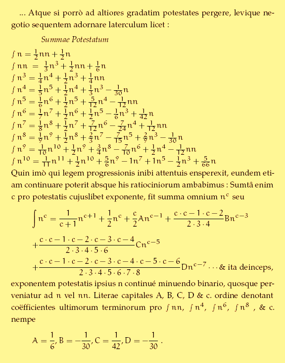
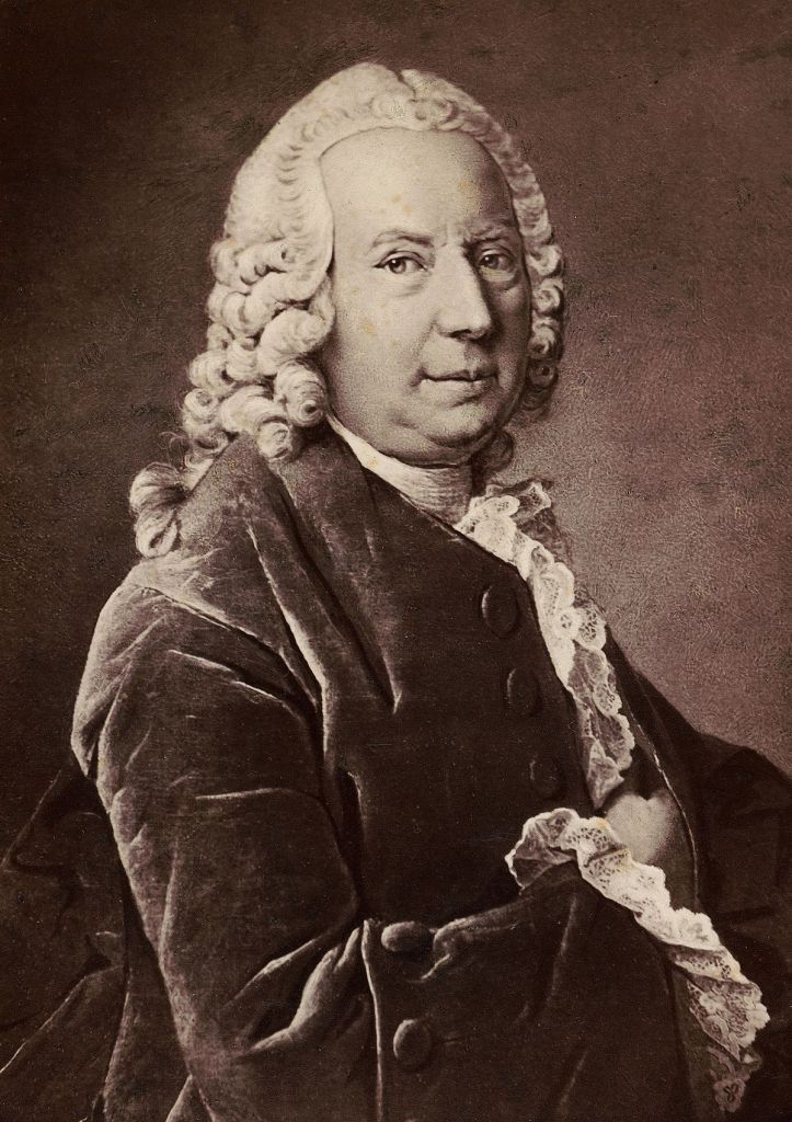
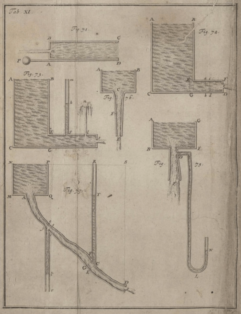
Daniel Bernoulli, the son of Johann I Bernoulli, was the first to study the double pendulum, publishing a paper on the topic in 1733 in the proceedings of the Academy in St. Petersburg just as he returned from Russia to take up a post permanently in his home town of Basel, Switzerland.  Because he was a physicist first and mathematician second, he performed experiments with masses on strings to attempt to understand the qualitative as well as quantitative behavior of the two-mass system.  He discovered that for small motions there was a symmetric behavior that had a low frequency of oscillation and an antisymmetric motion that had a higher frequency of oscillation.  Furthermore, he recognized that any general motion of the double pendulum was a combination of the fundamental symmetric and antisymmetric motions.  This work by Daniel Bernoulli represents the discovery of normal modes of coupled oscillators.  It is also the first statement of the combination of motions that he would use later (1753) to express for the first time the principle of superposition. 

Superposition is one of the guiding principles of linear physical systems.  It provides a means for the solution of differential equations.  It explains the existence of eigenmodes and their eigenfrequencies.  It is the basis of all interference phenomenon, whether classical like the Young’s double-slit experiment or quantum like Schrödinger’s cat.  Today, superposition has taken center stage in quantum information sciences and helps define the spooky (and useful) properties of quantum entanglement.  Therefore, normal modes, composition of motion, superposition of harmonics on a musical string—these all date back to Daniel Bernoulli in the twenty years between 1733 and 1753.  (Daniel Bernoulli is also the originator of the Bernoulli principle that explains why birds and airplanes fly.)

Johann Bernoulli and the Equations of Motion

Daniel Bernoulli’s father was Johann I Bernoulli.  Daniel had been tutored by Johann, along with his friend Leonhard Euler, when Daniel was young.  But as Daniel matured as a mathematician, he and his father began to compete against each other in international mathematics competitions (which were very common in the early eighteenth century).  When Daniel beat his father in a competition sponsored by the French Academy, Johann threw Daniel out of his house and their relationship remained strained for the remainder of their lives.

Johann had a history of taking ideas from Daniel and never citing the source. For instance, when Johann published his work on equations of motion for masses on strings in 1742, he built on the work of his son Daniel from 1733 but never once mentioned it. Daniel, of course, was not happy.

In a letter dated 20 October 1742 that Daniel wrote to Euler, he said, “The collected works of my father are being printed, and I have Just learned that he has inserted, without any mention of me, the dynamical problems I first discovered and solved (such as e. g. the descent of a sphere on a moving triangle; the linked pendulum, the center of spontaneous rotation, etc.).” And on 4 September 1743, when Daniel had finally seen his father’s works in print, he said, “The new mechanical problems are mostly mine, and my father saw my solutions before he solved the problems in his way …”. [2]

Daniel clearly has the priority for the discovery of the normal modes of the linked (i.e. double or compound) pendulum, but Johann often would “improve” on Daniel’s work despite giving no credit for the initial work. As a mathematician, Johann had a more rigorous approach and could delve a little deeper into the math. For this reason, it was Johann in 1742 who came closest to writing down differential equations of motion for multi-mass systems, but falling just short. It was D’Alembert only one year later who first wrote down the differential equations of motion for systems of masses and extended it to the loaded string for which he was the first to derive the wave equation. The D’Alembertian operator is today named after him.

Double Pendulum Dynamics

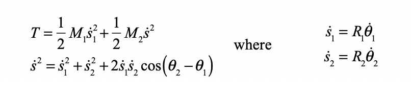
The general dynamics of the double pendulum are best obtained from Lagrange’s equations of motion. However, setting up the Lagrangian takes careful thought, because the kinetic energy of the second mass depends on its absolute speed which is dependent on the motion of the first mass from which it is suspended. The velocity of the second mass is obtained through vector addition of velocities.

Fig. 2. The dynamics of the double pendulum.

The potential energy of the system is

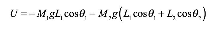
so that the Lagrangian is

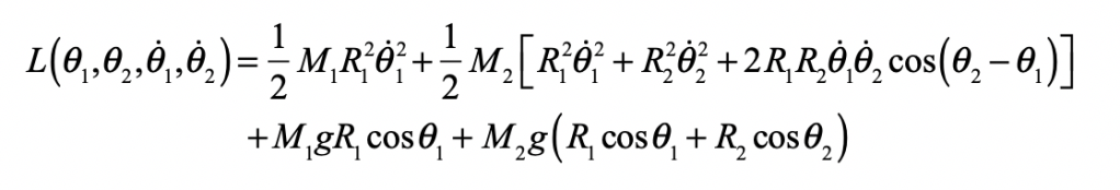
The partial derivatives are

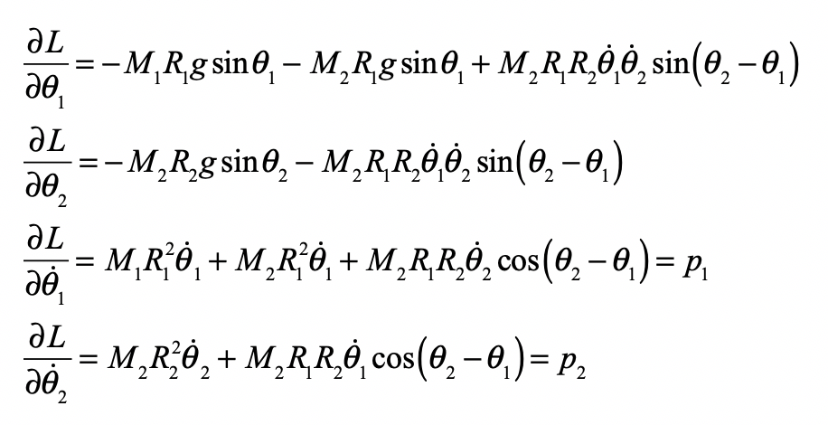
and the time derivatives of the last two expressions are

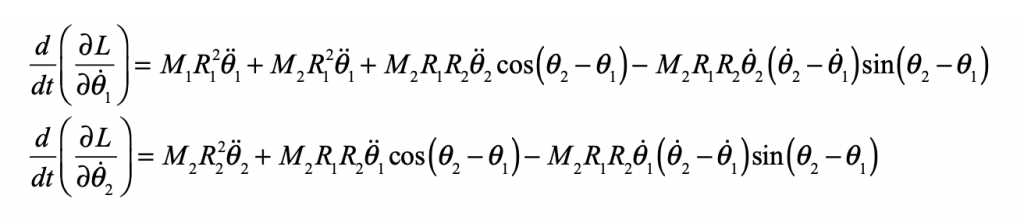
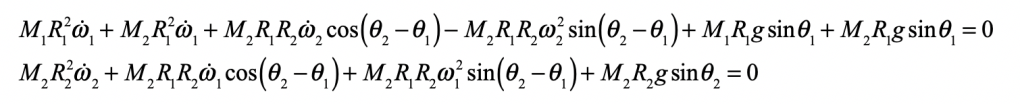
Therefore, the equations of motion are

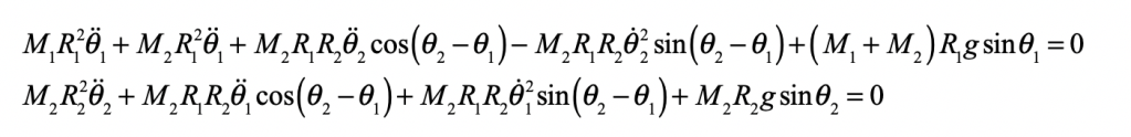
To get a sense of how this system behaves, we can make a small-angle approximation to linearize the equations to find the lowest-order normal modes.  In the small-angle approximation, the equations of motion become

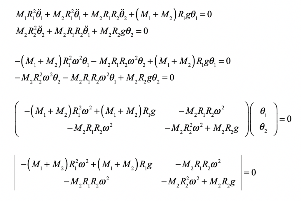
where the determinant is

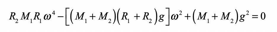
This quartic equation is quadratic in w2 and the quadratic solution is

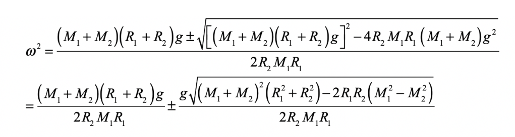
This solution is still a little opaque, so taking the special case: R = R1 = R2 and M = M1 = M2 it becomes

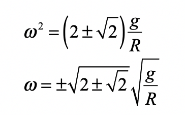
There are two normal modes.  The low-frequency mode is symmetric as both masses swing (mostly) together, while the higher frequency mode is antisymmetric with the two masses oscillating against each other.  These are the motions that Daniel Bernoulli discovered in 1733.

It is interesting to note that if the string were rigid, so that the two angles were the same, then the lowest frequency would be 3/5 which is within 2% of the above answer but is certainly not equal.  This tells us that there is a slightly different angular deflection for the second mass relative to the first.

Chaos in the Double Pendulum

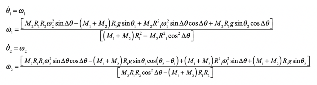
The full expression for the nonlinear coupled dynamics is expressed in terms of four variables (q1, q2, w1, w2).  The dynamical equations are

These can be put into the normal form for a four-dimensional flow as

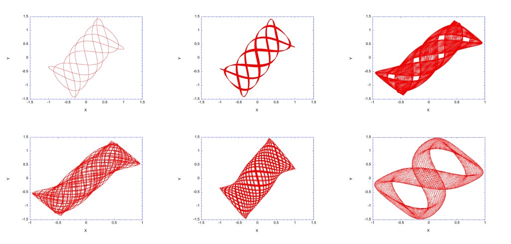
The numerical solution of these equations produce a complex interplay between the angle of the first mass and the angle of the second mass. Examples of trajectory projections in configuration space are shown in Fig. 3 for E = 1. The horizontal is the first angle, and the vertical is the angle of the second mass.

Fig. 3 Trajectory projections onto configuration space. The horizontal axis is the first mass angle, and the vertical axis is the second mass angle. All of these are periodic or nearly periodic orbits except for the one on the lower left. E = 1.

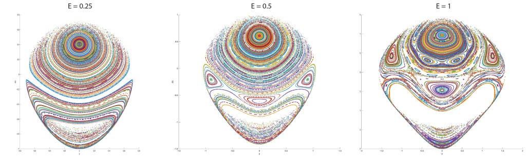
The dynamics in state space are four dimensional which are difficult to visualize directly. Using the technique of the Poincaré first-return map, the four-dimensional trajectories can be viewed as a two-dimensional plot where the trajectories pierce the Poincaré plane. Poincare sections are shown in Fig. 4.

Fig. Poincare sections of the double pendulum in state space for increasing kinetic energy. Initial conditions are vertical in all. The horizontal axis is the angle of the second mass, and the vertical axis is the angular velocity of the second mass.

Python Code: DoublePendulum.py

(Python code on GitHub.)

#!/usr/bin/env python3
# -*- coding: utf-8 -*-
"""
DoublePendulum.py
Created on Oct 16 06:03:32 2020
"Introduction to Modern Dynamics" 2nd Edition (Oxford, 2019)
@author: nolte
"""

import numpy as np
from scipy import integrate
from matplotlib import pyplot as plt
import time

plt.close('all')

E = 1.       # Try 0.8 to 1.5

def flow_deriv(x_y_z_w,tspan):
    x, y, z, w = x_y_z_w

    A = w**2*np.sin(y-x);
    B = -2*np.sin(x);
    C = z**2*np.sin(y-x)*np.cos(y-x);
    D = np.sin(y)*np.cos(y-x);
    EE = 2 - (np.cos(y-x))**2;
    
    FF = w**2*np.sin(y-x)*np.cos(y-x);
    G = -2*np.sin(x)*np.cos(y-x);
    H = 2*z**2*np.sin(y-x);
    I = 2*np.sin(y);
    JJ = (np.cos(y-x))**2 - 2;

    a = z
    b = w
    c = (A+B+C+D)/EE
    d = (FF+G+H+I)/JJ
    return[a,b,c,d]

repnum = 75

np.random.seed(1)
for reploop  in range(repnum):
    
    
    px1 = 2*(np.random.random((1))-0.499)*np.sqrt(E);
    py1 = -px1 + np.sqrt(2*E - px1**2);            

    xp1 = 0   # Try 0.1
    yp1 = 0   # Try -0.2
    
    x_y_z_w0 = [xp1, yp1, px1, py1]
    
    tspan = np.linspace(1,1000,10000)
    x_t = integrate.odeint(flow_deriv, x_y_z_w0, tspan)
    siztmp = np.shape(x_t)
    siz = siztmp[0]

    if reploop % 50 == 0:
        plt.figure(2)
        lines = plt.plot(x_t[:,0],x_t[:,1])
        plt.setp(lines, linewidth=0.5)
        plt.show()
        time.sleep(0.1)
        #os.system("pause")

    y1 = np.mod(x_t[:,0]+np.pi,2*np.pi) - np.pi
    y2 = np.mod(x_t[:,1]+np.pi,2*np.pi) - np.pi
    y3 = np.mod(x_t[:,2]+np.pi,2*np.pi) - np.pi
    y4 = np.mod(x_t[:,3]+np.pi,2*np.pi) - np.pi
    
    py = np.zeros(shape=(10*repnum,))
    yvar = np.zeros(shape=(10*repnum,))
    cnt = -1
    last = y1[1]
    for loop in range(2,siz):
        if (last < 0)and(y1[loop] > 0):
            cnt = cnt+1
            del1 = -y1[loop-1]/(y1[loop] - y1[loop-1])
            py[cnt] = y4[loop-1] + del1*(y4[loop]-y4[loop-1])
            yvar[cnt] = y2[loop-1] + del1*(y2[loop]-y2[loop-1])
            last = y1[loop]
        else:
            last = y1[loop]
     
    plt.figure(3)
    lines = plt.plot(yvar,py,'o',ms=1)
    plt.show()
    
plt.savefig('DPen')

You can change the energy E on line 16 and also the initial conditions xp1 and yp1 on lines 48 and 49. The energy E is the initial kinetic energy imparted to the two masses. For a given initial condition, what happens to the periodic orbits as the energy E increases?

References

[1] Daniel Bernoulli, Theoremata de oscillationibus corporum filo flexili connexorum et catenae verticaliter suspensae,” Academiae Scientiarum Imperialis Petropolitanae, 6, 1732/1733

[2] Truesdell B. The rational mechanics of flexible or elastic bodies, 1638-1788. (Turici: O. Fussli, 1960). (This rare and artistically produced volume, that is almost impossible to find today in any library, is one of the greatest books written about the early history of dynamics.)

The Bountiful Bernoullis of Basel

The task of figuring out who’s who in the Bernoulli family is a hard nut to crack.  The Bernoulli name populates a dozen different theorems or physical principles in the history of science and mathematics, but each one was contributed by any of four or five different Bernoullis of different generations—brothers, uncles, nephews and cousins.  What makes the task even more difficult is that any given Bernoulli might be called by several different aliases, while many of them shared the same name across generations.  To make things worse, they often worked and published on each other’s problems.

To attribute a theorem to a Bernoulli is not too different from attributing something to the famous mathematical consortium called Nicholas Bourbaki.  It’s more like a team rather than an individual.  But in the case of Bourbaki, the goal was selfless anonymity, while in the case of the Bernoullis it was sometimes the opposite—bald-faced competition and one-up-manship coupled with jealousy and resentment. Fortunately, the competition tended to breed more output than less, and the world benefited from the family feud.

The Bernoulli Family Tree

The Bernoullis are intimately linked with the beautiful city of Basel, Switzerland, situated on the Rhine River where it leaves Switzerland and forms the border between France and Germany . The family moved there from the Netherlands in the 1600’s to escape the Spanish occupation.

Basel Switzerland

The first Bernoulli born in Basel was Nikolaus Bernoulli (1623 – 1708), and he had four sons: Jakob I, Nikolaus, Johann I and Hieronymous I. The “I”s in this list refer to the fact, or the problem, that many of the immediate descendants took their father’s or uncle’s name. The long-lived family heritage in the roles of mathematician and scientist began with these four brothers. Jakob Bernoulli (1654 – 1705) was the eldest, followed by Nikolaus Bernoulli (1662 – 1717), Johann Bernoulli (1667 – 1748) and then Hieronymous (1669 – 1760). In this first generation of Bernoullis, the great mathematicians were Jakob and Johann. More mathematical equations today are named after Jakob, but Johann stands out because of the longevity of his contributions, the volume and impact of his correspondence, the fame of his students, and the number of offspring who also took up mathematics. Johann was also the worst when it came to jealousy and spitefulness—against his brother Jakob, whom he envied, and specifically against his son Daniel, whom he feared would eclipse him.

Jakob Bernoulli (aka James or Jacques or Jacob)

Jakob Bernoulli (1654 – 1705) was the eldest of the first generation of brothers and also the first to establish himself as a university professor. He held the chair of mathematics at the university in Basel. While his interests ranged broadly, he is known for his correspondences with Leibniz as he and his brother Johann were among the first mathematicians to apply Lebiniz’ calculus to solving specific problems. The Bernoulli differential equation is named after him. It was one of the first general differential equations to be solved after the invention of the calculus. The Bernoulli inequality is one of the earliest attempts to find the Taylor expansion of exponentiation, which is also related to Bernoulli numbers, Bernoulli polynomials and the Bernoulli triangle. A special type of curve that looks like an ellipse with a twist in the middle is the lemniscate of Bernoulli.

Perhaps Jakob’s most famous work was his Ars Conjectandi (1713) on probability theory. Many mathematical theorems of probability named after a Bernoulli refer to this work, such as Bernoulli distribution, Bernoulli’s golden theorem (the law of large numbers), Bernoulli process and Bernoulli trial.

Fig. Bernoulli numbers in Jakob’s Ars Conjectandi (1713)

Johann Bernoulli (aka Jean or John)

Jakob was 13 years older than his brother Johann Bernoulli (1667 – 1748), and Jakob tutored Johann in mathematics who showed great promise. Unfortunately, Johann had that awkward combination of high self esteem with low self confidence, and he increasingly sought to show that he was better than his older brother. As both brothers began corresponding with Leibniz on the new calculus, they also began to compete with one another. Driven by his insecurity, Johann also began to steal ideas from his older brother and claim them for himself.

A classic example of this is the famous brachistrochrone problem that was posed by Johann in the Acta Eruditorum in 1696. Johann at this time was a professor of mathematics at Gronigen in the Netherlands. He challenged the mathematical world to find the path of least time for a mass to travel under gravity between two points. He had already found one solution himself and thought that no-one else would succeed. Yet when he heard his brother Jakob was responding to the challenge, he spied out his result and then claimed it as his own. Within the year and a half there were 4 additional solutions—all correct—using different approaches.  One of the most famous responses was by Newton (who as usual did not give up his method) but who is reported to have solved the problem in a day.  Others who contributed solutions were Gottfried Leibniz, Ehrenfried Walther von Tschirnhaus, and Guillaume de l’Hôpital in addition to Jakob.

The participation of de l’Hôpital in the challenge was a particular thorn in Johann’s side, because de l’Hôpital had years earlier paid Johann to tutor him in Leibniz’ new calculus at a time when l’Hôpital knew nothing of the topic. What is today known as l’Hôpital’s theorem on ratios of limits in fact was taught to l’Hôpital by Johann. Johann never forgave l’Hôpital for publicizing the result—but l’Hôpital had the discipline to write a textbook while Johann did not. To be fair, l’Hôpital did give Johann credit in the opening of his book, but that was not enough for Johann who continued to carry his resentment.

When Jakob died of tuberculosis in 1705, Johann campaigned to replace him in his position as professor of mathematics and succeeded. In that chair, Johann had many famous students (Euler foremost among them, but also Maupertuis and Clairaut). Part of Johann’s enduring fame stems from his many associations and extensive correspondences with many of the top mathematicians of the day. For instance, he had a regular correspondence with the mathematician Varignon, and it was in one of these letters that Johann proposed the principle of virtual velocities which became a key axiom for Joseph Lagrange’s later epic work on the foundations of mechanics (see Chapter 4 in Galileo Unbound).

Johann remained in his chair of mathematics at Basel for almost 40 years. This longevity, and the fame of his name, guaranteed that he taught some of the most talented mathematicians of the age, including his most famous student Leonhard Euler, who is held by some as one of the four greatest mathematicians of all time (the others were Archimedes, Newton and Gauss) [1].

Nikolaus I Bernoulli

Nikolaus I Bernoulli (1687 – 1759, son of Nikolaus) was the cousin of Daniel and nephew to both Jacob and Johann. He was a well-known mathematician in his time (he briefly held Galileo’s chair in Padua), though few specific discoveries are attributed to him directly. He is perhaps most famous today for posing the “St. Petersburg Paradox” of economic game theory. Ironically, he posed this paradox while his cousin Nikolaus II Bernoulli (brother of Daniel Bernoulli) was actually in St. Petersburg with Daniel.

The St. Petersburg paradox is a simple game of chance played with a fair coin where a player must buy in at a certain price in order to place $2 in a pot that doubles each time the coin lands heads, and pays out the pot at the first tail. The average pay-out of this game has infinite expectation, so it seems that anyone should want to buy in at any cost. But most people would be unlikely to buy in even for a modest $25. Why? And is this perception correct? The answer was only partially provided by Nikolaus. The definitive answer was given by his cousin Daniel Bernoulli.

Daniel Bernoulli

Daniel Bernoulli (1700 – 1782, son of Johann I) is my favorite Bernoulli. While most of the other Bernoullis were more mathematicians than scientists, Daniel Bernoulli was more physicist than mathematician. When we speak of “Bernoulli’s principle” today, the fundamental force that allows birds and airplanes to fly, we are referring to his work on hydrodynamics. He was one of the earliest originators of economic dynamics through his invention of the utility function and diminishing returns, and he was the first to clearly state the principle of superposition, which lies at the heart today of the physics of waves and quantum technology.

Daniel Bernoulli

While in St. Petersburg, Daniel conceived of the solution to the St. Petersburg paradox (he is the one who actually named it). To explain why few people would pay high stakes to play the game, he devised a “utility function” that had “diminishing marginal utility” in which the willingness to play depended on ones wealth. Obviously a wealthy person would be willing to pay more than a poor person. Daniel stated

The determination of the value of an item must not be based on the price, but rather on the utility it yields…. There is no doubt that a gain of one thousand ducats is more significant to the pauper than to a rich man though both gain the same amount.

He created a log utility function that allowed one to calculate the highest stakes a person should be willing to take based on their wealth. Indeed, a millionaire may only wish to pay $20 per game to play, in part because the average payout over a few thousand games is only about $5 per game. It is only in the limit of an infinite number of games (and an infinite bank account by the casino) that the average payout diverges.

Daniel Bernoulli Hydrodynamica (1638)

Johann II Bernoulli

Daniel’s brother Johann II (1710 – 1790) published in 1736 one of the most important texts on the theory of light during the time between Newton and Euler. Although the work looks woefully anachronistic today, it provided one of the first serious attempts at understanding the forces acting on light rays and describing them mathematically [5]. Euler based his new theory of light, published in 1746, on much of the work laid down by Johann II. Euler came very close to proposing a wave-like theory of light, complete with a connection between frequency of wave pulses and colors, that would have preempted Thomas Young by more than 50 years. Euler, Daniel and Johann II as well as Nicholas II were all contemporaries as students of Johann I in Basel.

More Relations

Over the years, there were many more Bernoullis who followed in the family tradition. Some of these include:

Johann II Bernoulli (1710–1790; also known as Jean), son of Johann, mathematician and physicist

Johann III Bernoulli (1744–1807; also known as Jean), son of Johann II, astronomer, geographer and mathematician

Jacob II Bernoulli (1759–1789; also known as Jacques), son of Johann II, physicist and mathematician

Johann Jakob Bernoulli (1831–1913), art historian and archaeologist; noted for his Römische Ikonographie (1882 onwards) on Roman Imperial portraits

Ludwig Bernoully (1873 – 1928), German architect in Frankfurt

Hans Bernoulli (1876–1959), architect and designer of the Bernoullihäuser in Zurich and Grenchen SO

Elisabeth Bernoulli (1873-1935), suffragette and campaigner against alcoholism.

Notable marriages to the Bernoulli family include the Curies (Pierre Curie was a direct descendant to Johann I) as well as the German author Hermann Hesse (married to a direct descendant of Johann I).

References

[1] Calinger, Ronald S.. Leonhard Euler : Mathematical Genius in the Enlightenment, Princeton University Press (2015).

[2] Euler L and Truesdell C. Leonhardi Euleri Opera Omnia. Series secunda: Opera mechanica et astronomica XI/2. The rational mechanics of flexible or elastic bodies 1638-1788. (Zürich: Orell Füssli, 1960).

[3] D Speiser, Daniel Bernoulli (1700-1782), Helvetica Physica Acta 55 (1982), 504-523.

[4] Leibniz GW. Briefwechsel zwischen Leibniz, Jacob Bernoulli, Johann Bernoulli und Nicolaus Bernoulli. (Hildesheim: Olms, 1971).

[5] Hakfoort C. Optics in the age of Euler : conceptions of the nature of light, 1700-1795. (Cambridge: Cambridge University Press, 1995).