
Hamiltonian systems are freaks of nature. Unlike the everyday world we experience that is full of dissipation and inefficiency, Hamiltonian systems live in a world free of loss. Despite how rare this situation is for us, this unnatural state happens commonly in two extremes: orbital mechanics and quantum mechanics. In the case of orbital mechanics, dissipation does exist, most commonly in tidal effects, but effects of dissipation in the orbits of moons and planets takes eons to accumulate, making these systems effectively free of dissipation on shorter time scales. Quantum mechanics is strictly free of dissipation, but there is a strong caveat: ALL quantum states need to be included in the quantum description. This includes the coupling of discrete quantum states to their environment. Although it is possible to isolate quantum systems to a large degree, it is never possible to isolate them completely, and they do interact with the quantum states of their environment, if even just the black-body radiation from their container, and even if that container is cooled to milliKelvins. Such interactions involve so many degrees of freedom, that it all behaves like dissipation. The origin of quantum decoherence, which poses such a challenge for practical quantum computers, is the entanglement of quantum systems with their environment.
Liouville’s theorem plays a central role in the explanation of the entropy and ergodic properties of ideal gases, as well as in Hamiltonian chaos.
Liouville’s Theorem and Phase Space
A middle ground of practically ideal Hamiltonian mechanics can be found in the dynamics of ideal gases. This is the arena where Maxwell and Boltzmann first developed their theories of statistical mechanics using Hamiltonian physics to describe the large numbers of particles. Boltzmann applied a result he learned from Jacobi’s Principle of the Last Multiplier to show that a volume of phase space is conserved despite the large number of degrees of freedom and the large number of collisions that take place. This was the first derivation of what is today known as Liouville’s theorem.
In 1838 Joseph Liouville, a pure mathematician, was interested in classes of solutions of differential equations. In a short paper, he showed that for one class of differential equation one could define a property that remained invariant under the time evolution of the system. This purely mathematical paper by Liouville was expanded upon by Jacobi, who was a major commentator on Hamilton’s new theory of dynamics, contributing much of the mathematical structure that we associate today with Hamiltonian mechanics. Jacobi recognized that Hamilton’s equations were of the same class as the ones studied by Liouville, and the conserved property was a product of differentials. In the mid-1800’s the language of multidimensional spaces had yet to be invented, so Jacobi did not recognize the conserved quantity as a volume element, nor the space within which the dynamics occurred as a space. Boltzmann recognized both, and he was the first to establish the principle of conservation of phase space volume. He named this principle after Liouville, even though it was actually Boltzmann himself who found its natural place within the physics of Hamiltonian systems [1].
Liouville’s theorem plays a central role in the explanation of the entropy of ideal gases, as well as in Hamiltonian chaos. In a system with numerous degrees of freedom, a small volume of initial conditions is stretched and folded by the dynamical equations as the system evolves. The stretching and folding is like what happens to dough in a bakers hands. The volume of the dough never changes, but after a long time, a small spot of food coloring will eventually be as close to any part of the dough as you wish. This analogy is part of the motivation for ergodic systems, and this kind of mixing is characteristic of Hamiltonian systems, in which trajectories can diffuse throughout the phase space volume … usually.
Interestingly, when the number of degrees of freedom are not so large, there is a middle ground of Hamiltonian systems for which some initial conditions can lead to chaotic trajectories, while other initial conditions can produce completely regular behavior. For the right kind of systems, the regular behavior can hem in the irregular behavior, restricting it to finite regions. This was a major finding of the KAM theory [2], named after Kolmogorov, Arnold and Moser, which helped explain the regions of regular motion separating regions of chaotic motion as illustrated in Chirikov’s Standard Map.
Discrete Maps
Hamilton’s equations are ordinary continuous differential equations that define a Hamiltonian flow in phase space. These equations can be solved using standard techniques, such as Runge-Kutta. However, a much simpler approach for exploring Hamiltonian chaos uses discrete maps that represent the Poincaré first-return map, also known as the Poincaré section. Testing that a discrete map satisfies Liouville’s theorem is as simple as checking that the determinant of the Floquet matrix is equal to unity. When the dynamics are represented in a Poincaré plane, these maps are called area-preserving maps.
There are many famous examples of area-preserving maps in the plane. The Chirikov Standard Map is one of the best known and is often used to illustrate KAM theory. It is a discrete representation of a kicked rotater, while a kicked harmonic oscillator leads to the Web Map. The Henon Map was developed to explain the orbits of stars in galaxies. The Lozi Map is a version of the Henon map that is more accessible analytically. And the Cat Map was devised by Vladimir Arnold to illustrate what is today called Arnold Diffusion. All of these maps display classic signatures of (low-dimensional) Hamiltonian chaos with periodic orbits hemming in regions of chaotic orbits.
| Chirikov Standard Map | Kicked rotater |
| Web Map | Kicked harmonic oscillator |
| Henon Map | Stellar trajectories in galaxies |
| Lozi Map | Simplified Henon map |
| Cat Map | Arnold Diffusion |
Table: Common examples of area-preserving maps.
Lozi Map
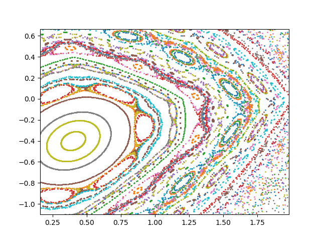
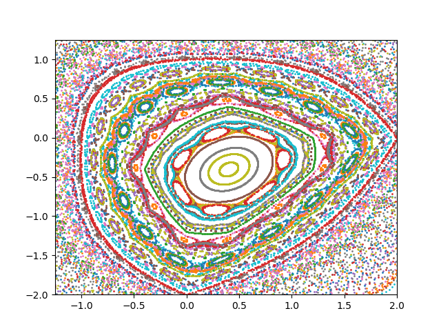
My favorite area-preserving discrete map is the Lozi Map. I first stumbled on this map at the very back of Steven Strogatz’ wonderful book on nonlinear dynamics [3]. It’s one of the last exercises of the last chapter. The map is particularly simple, but it leads to rich dynamics, both regular and chaotic. The map equations are
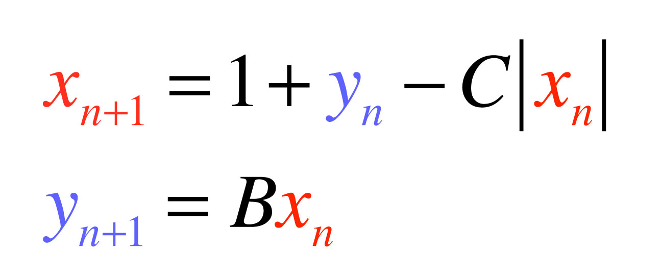
which is area-preserving when |B| = 1. The constant C can be varied, but the choice C = 0.5 works nicely, and B = -1 produces a beautiful nested structure, as shown in the figure.
Python Code for the Lozi Map
"""
Lozi.py
Created on Wed May  2 16:17:27 2018
@author: nolte
"""
import numpy as np
from scipy import integrate
from matplotlib import pyplot as plt

B = -1
C = 0.5

np.random.seed(2)
plt.figure(1)

for eloop in range(0,100):

    xlast = np.random.normal(0,1,1)
    ylast = np.random.normal(0,1,1)

    xnew = np.zeros(shape=(500,))
    ynew = np.zeros(shape=(500,))
    for loop in range(0,500):
        xnew[loop] = 1 + ylast - C*abs(xlast)
        ynew[loop] = B*xlast
        xlast = xnew[loop]
        ylast = ynew[loop]

    plt.plot(np.real(xnew),np.real(ynew),'o',ms=1)
    plt.xlim(xmin=-1.25,xmax=2)
    plt.ylim(ymin=-2,ymax=1.25)

plt.savefig('Lozi')
References:
[1] D. D. Nolte, “The Tangled Tale of Phase Space”, Chapter 6 in Galileo Unbound: A Path Across Life, the Universe and Everything (Oxford University Press, 2018)
[2] H. S. Dumas, The KAM Story: A Friendly Introduction to the Content, History, and Significance of Classical Kolmogorov-Arnold-Moser Theory (World Scientific, 2014)
[3] S. H. Strogatz, Nonlinear Dynamics and Chaos (WestView Press, 1994)
